Quantum-dot thermometry

Abstract

We present a method for the measurement of a temperature differential across a single quantum dot that has transmission resonances that are separated in energy by much more than the thermal energy. We determine numerically that the method is accurate to within a few percent across a wide range of parameters. The proposed method measures the temperature of the electrons that enter the quantum dot and will be useful in experiments that aim to test theory which predicts quantum dots are highly efficient thermoelectrics.

In the ongoing development of effective thermoelectric materials and devices, low-dimensional systems are of particularly great interest, because to optimize the performance of a thermoelectric, it is crucial to control the energy spectrum of mobile electrons Hicks and Dresselhaus (1993); Mahan and Sofo (1996); Humphrey et al. (2002, 2005); Humphrey and Linke (2005). Devices for high-efficiency thermal-to-electric power conversion based on quantum dots defined by double barriers embedded in nanowires have been proposed O’Dwyer et al. (2006). Such systems have great advantages, because they select the energies at which electrons are transmitted Björk et al. (2002, 2004), and because nanowires can be contacted in highly ordered arrays Bryllert et al. (2006) with the potential for large-scale parallel operation.

In order to measure quantitatively the dependence of thermopower and energy-conversion efficiency on the transmission spectrum of a quantum dot, it is necessary to apply and determine accurately a temperature differential across the dot. Traditionally for the thermoelectric characterization of mesoscopic devices such as quantum point contacts Molenkamp et al. (1992), quantum dots in 2DEG’s Molenkamp et al. (1994), carbon nanotubes Hone et al. (1998); Small et al. (2003); Llaguno et al. (2004), and nanowires Seol et al. (2007); Shi et al. (2003), an ac heating current generates a temperature differential that is measured in separate calibration experiments. Here we propose a technique that measures the actual electronic temperature differential across a quantum dot and does not require separate calibration. The basic concept is as follows: the change in current across a quantum dot in response to an applied heating voltage, $V_{\text{H}}$, is measured. This signal contains information about the electron temperatures at the source and drain, but it also depends on the dot’s energy-dependent transmission function, $\tau\left(\varepsilon\right)$. However, one can obtain the necessary information about $\tau\left(\varepsilon\right)$ from conductance measurements. Together, these two measurements allow one to determine the source and drain temperatures separately.

The two-terminal current through a quantum dot can be written Landauer (1957, 1970)

$$I=\frac{2e}{h}\int_{-\infty}^{\infty}\left[f_{\text{s}}\left(\varepsilon\right)-f_{\text{d}}\left(\varepsilon\right)\right]\tau\left(\varepsilon\right)d\varepsilon,$$ (1)

where $f_{\text{s,d}}^{-1}=e^{\xi_{\text{s,d}}}+1$ are the Fermi-Dirac distributions in the nanowire’s source and drain leads, respectively, and their arguments are $\xi_{\text{s,d}}=\left(\varepsilon-\mu_{\text{s,d}}\mp eV/2\right)/k_{\text{B}}T_{\text{s,d}}$. We assume the bias voltage, $V$, is applied symmetrically across the dot. For the case of a quantum dot or single-electron transistor (SET) with well-separated transmission maxima as a function of gate voltage, Eq. (1) predicts the characteristic Coulomb blockade diamonds which appear in the differential conductance, $G$, as a function of bias voltage and gate voltage.

Figure 1: The heating setup and the temperature landscape. The source contact is warmed with a voltage-balanced heating current and can be biased for thermocurrent measurements. Electron transport through the quantum dot is determined by the local temperatures of the source and drain sides of the dot, $T_{\text{ s,d}}=\Delta T_{\text{s,d}}+T_{\text{0}}$. (Color online)

In a typical experiment, an ac heating current is used to modulate the temperature $T_{\text{H}}$ of an ohmic contact at one end of a nanowire (taken here to be the source contact, Fig. 1)foo with amplitude $\Delta T_{\text{H}}$ with respect to the unperturbed device temperature, $T_{\text{0}}$. We are interested in the associated electronic temperature rises, $\Delta T_{\text{s,d}}=T_{\text{s,d}}-T_{0}$, in the immediate vicinity of the quantum dot (see Fig. 1). In the case of strong electron- phonon interaction (for example near room temperature) the electronic temperature will drop linearly along the nanowire, and $\Delta T_{\text{s}}\cong\Delta T_{\text{d}}$ if the quantum dot is short compared to the wire. At low temperatures, however, where electron-phonon interaction in the nanowire is expected to be weak, $\Delta T_{\text{H}}>\Delta T_{\text{s }}>\Delta T_{\text{d}}>0$, and $\Delta T_{\text{s}}$ and $\Delta T_{\text{ d}}$ need to be measured.

Assuming an ac heating voltage, $V_{\text{H}}=V_{\text{0}}\cos(\omega t$), the temperature rises on the source and drain sides of the dot can be written $\Delta T_{\text{s,d}}=\beta_{\text{s,d}}V_{\text{H}}^{\gamma}$ , where $\beta_{\text{s,d}}$ are unknown constants and $\gamma$ can take on various values depending on the type and strength of electron-phonon interaction in the heating wire Henny et al. (1997). Here we assume a short heating wire and Joule heating, and therefore $\gamma=2$ Henny et al. (1997). In this regime, by an application of the chain rule, the rms-amplitude of the ac temperature rises can be written

$$\Delta T_{\text{s,d}}\cong V_{0}^{2}\frac{\partial T_{\text{s,d }}}{\partial\left(V_{\text{H}}^{2}\right)}=V_{0}^{2}\left(\frac{\partial I}{\partial T_{\text{s,d}}}\right)^{-1}\frac{\partial I}{\partial\left(V_{\text{H}}^{2}\right)}.$$ (2)

In an experiment, one can measure $\partial I/\partial\left(V_{\text{H}}^{2}\right)$, the frequency-doubled response to the ac heating voltage. The differential thermocurrent,

$$\frac{\partial I}{\partial T_{\text{s,d}}}=\frac{2e}{h}\int_{-\infty}^{\infty}\left(\mp\frac{\partial f_{\text{s,d}}}{\partial\xi_{\text{ s,d }}}\frac{\xi_{\text{s,d}}}{T_{\text{s,d}}}\right)\tau\left(\varepsilon\right)d\varepsilon,$$ (3)

cannot be measured directly.  However, we will show that it can be obtained in good approximation from conductance measurements.

Under bias conditions, where the source (drain) electrochemical potential is near a well-defined transmission resonance of the quantum dot, while the drain (source) is several $k_{\text{B}}T$ away from the next resonance, the second derivative of the current is

$$\frac{\partial^{2}I}{\partial V^{2}}\cong\frac{e^{2}}{4k_{\text{B}}^{2}}\frac{1}{T_{\text{s,d}}}\frac{2e}{h}\int_{-\infty}^{\infty}\left(\pm\frac{\partial f_{\text{s,d}}}{\partial\xi_{\text{s,d}}}\frac{2f_{\text{ s,d }}-1}{T_{\text{s,d}}}\right)\tau\left(\varepsilon\right)d\varepsilon.$$ (4)

A key observation is that the integrands in Eq. (3) and Eq. ( 4) are qualitatively very similar:

$$\frac{\partial f_{\text{s,d}}}{\partial\xi_{\text{s,d}}}\frac{2f_{\text{ s,d }}-1}{T_{\text{s,d}}}\cong-\frac{1}{2}\frac{\partial f_{\text{s,d}}}{\partial\xi_{\text{s,d}}}\frac{\xi_{\text{s,d}}}{T_{\text{s,d}}}.$$ (5)

This approximation holds for all $\xi_{\text{s,d}}$, because $2f_{\text{s,d}}-1$ limits to $-\xi_{\text{s,d}}/2$ when $\xi_{\text{s,d}}$ is small, and $\partial f_{\text{s,d}}/\partial\xi_{\text{s,d}}$ goes to zero in all other cases.  With this approximation, we can combine Eqs. (3 ) and (4):

$$\frac{\partial I}{\partial T_{\text{s,d}}}\cong\left(\Lambda\frac{e^{2}}{4k_{\text{B}}^{2}}\frac{1}{T_{\text{s,d}}}\right)^{-1}\frac{\partial^{2}I}{\partial V^{2}},$$ (6)

where $\Lambda$ is a unitless scaling factor introduced during integration. In this way, all the information about $\tau\left(\varepsilon\right)$ needed to determine $\partial I/\partial T_{\text{s,d}}$ is accounted for by measuring $\partial^{2}I/\partial V^{2}$.

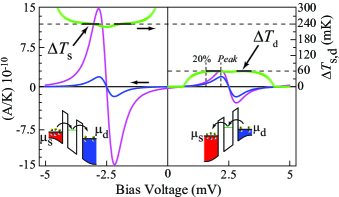
Figure 2: A plot of $\partial I/\partial T_{H}$ (red) and $(2k_{\text{B}}/e)^{2}\Delta T_{\text{H}}\partial^{2}I/\partial V^{2}$ (blue) as a function of bias voltage at a fixed gate voltage, as indicated by the horizontal dashed line in Fig. 3. The temperature rise (green) is calculated via Eq. (7). Insets: The position of the resonant tunneling energy of the dot with respect to the electrochemical potentials in the leads. In this model, we used a transmission function consisting of Lorentzians with a FWHM of $\Gamma=0.5$ meV equally spaced by 5 meV and $\Delta T_{\text{H}}=300$ mK, $\Delta T_{\text{s}}=0.8\Delta T_{\text{H}}$ $=240$ mK, $\Delta T_{\text{d}}=0.2\Delta T_{\text{H}}$ $=60$ mK, and $T_{\text{0}}=230$ mK. (Color online)

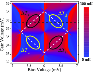
Figure 3: The calculated temperature rise as a function of bias and gate voltages for a single Coulomb blockade diamond. In the regions indicated, either the source or drain electrochemical potential, but not both, is within a few $k_{\text{B}}T$ of a resonant energy of the dot. Our assumptions are fulfilled in these regions, and the simulation produces temperature plateaus predicting the correct $\Delta T_{\text{s,d}}$. Fig. 2 shows a slice at 36.75 mV gate voltage, as indicated by the dashed line. (Color online)

Substituting Eq. (6) into Eq. (2) and solving for $\Delta T_{\text{s,d}}$ yields our final result,

$$\Delta T_{\text{s,d}}=\dfrac{1}{2}\sqrt{T_{\text{0}}^{2}+\Lambda\dfrac{e^{2}}{k_{\text{B}}^{2}}V_{\text{0}}^{2}\left(\frac{\partial^{2}I}{\partial V^{2}}\right)^{-1}\dfrac{\partial I}{\partial\left(V_{\text{H}}^{2}\right)}}-\dfrac{T_{\text{0}}}{2},$$ (7)

which shows that approximations of $\Delta T_{\text{s}}$ and $\Delta T_{\text{d}}$ can be obtained from measurement of $\partial^{2}I/\partial V^{2}$ and $\partial I/\partial\left(V_{\text{H}}^{2}\right)$ and knowledge of $T_{0}$.

To illustrate the qualitative similarity of Eqs. (3) and (4), we show numerical calculations of the two in Fig. 2 taken at the gate voltage indicated by the horizontal dashed line in Fig. 3 at 36.75 mV. The left inset of Fig. 2 illustrates that, in this example, when the bias voltage is negative, the source temperature is the only temperature affecting the current through the dot; therefore, $\partial I/\partial T_{\text{H}}=\partial I/\partial T_{\text{s}}$ in this bias configuration. In the opposite configuration, $\partial I/\partial T_{\text{H}}=\partial I/\partial T_{\text{d}}$, as shown in the right inset of Fig. 2. Fig. 3 shows Eq. (7) as calculated from modeled data of Eqs. (3) and (4) across an entire Coulomb blockade diamond (indicated by a white, dashed line), and a slice through that diamond is shown as green symbols in Fig. 2. In regions along the diamond ridges (circled areas in Fig. 3)—where one, and only one, of the two electrochemical potentials in the source or drain is within a few $k_{\text{B}}T$ of a transmission resonance—Eq. (7) yields consistent values in accordance with the assumptions that allow us to write Eq. (4). In all other regions, Eq. (4) is not valid, not even approximately, because it only accounts for one Fermi-Dirac distribution.

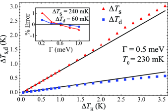
Figure 4: The calculated temperature rises as a function of $\Delta T_{\text{ H }}.$ The calculated values agree well with the expected values (solid lines) up to nearly 10 $T_{\text{0}}.$ Inset: The percent error as a function of $\Gamma$, the full width at half max (FWHM) of the transmission function, $\tau\left(\varepsilon\right)$ in Eq. (1). The error is within 1% over an order of magnitude in $\Gamma$. Here $\Delta T_{\text{s}}$ is 240 mK and $\Delta T_{\text{d}}$ is 60 mK. (Color online)

The use of this method requires knowledge of the appropriate scaling factor $\Lambda$, defined in Eq. 6, which needs to be determined numerically. For the particular modeling parameters used here (see caption of Fig. 2), we found $\Lambda=0.304$ by averaging Eq. (7) over the voltage range from the peak value of $\partial I/\partial T_{\text{H}}$ to 20% of its peak value, where the signal-to-noise ratio in an experiment should be largest. Note that for different parameters, $\Lambda$ will differ, but it is insensitive to typical experimental variations in $\Gamma$ and $\Delta T_{\text{H}}$. For example, in Fig. 4, we show that the use of the same $\Lambda=0.304$ (calculated for $\Gamma=0.5$ meV) yields errors in $\Delta T_{\text{s}}$ and $\Delta T_{\text{d}}$ of only 1% when $\Gamma$ is varied over nearly an order of magnitude around $\Gamma=0.5$ meV (inset of Fig. 4) and only a few percent for $\Delta T_{\text{H}}$ up to almost 10 $T_{\text{0}}$. To put this small error into context, note that the local temperatures $T_{\text{s}}$ and $T_{\text{d }}$ can be defined only over a distance of about an inelastic scattering length, such that an accuracy of less than a few percent is not necessarily physically meaningful.

This research was supported by ONR, ONR Global, the Swedish Research Council (VR), the Foundation for Strategic Research (SSF), the Knut and Alice Wallenberg Foundation, and an NSF-IGERT Fellowship.

References

- Hicks and Dresselhaus (1993) L. D. Hicks and M. S. Dresselhaus, Phys. Rev. B 47, 12727 (1993).
- Mahan and Sofo (1996) G. D. Mahan and J. O. Sofo, Proc. Natl. Acad. Sci. USA 93, 7436 (1996).
- Humphrey et al. (2002) T. E. Humphrey, R. Newbury, R. P. Taylor, and H. Linke, Phys. Rev. Lett. 89, 116801 (2002).
- Humphrey et al. (2005) T. E. Humphrey, M. F. O’Dwyer, and H. Linke, J. Phys. D 38, 2051 (2005).
- Humphrey and Linke (2005) T. E. Humphrey and H. Linke, Phys. Rev. Lett. 94, 096601 (2005).
- O’Dwyer et al. (2006) M. F. O’Dwyer, T. E. Humphrey, and H. Linke, Nanotech. 17, S338 (2006).
- Björk et al. (2002) M. T. Björk, B. J. Ohlsson, T. Sass, A. I. Persson, C. Thelander, M. H. Magnusson, K. Deppert, L. R. Wallenberg, and L. Samuelson, Nano Lett. 2, 87 (2002).
- Björk et al. (2004) M. T. Björk, C. Thelander, A. E. Hansen, L. E. Jensen, M. W. Larsson, L. R. Wallenberg, and L. Samuelson, Nano Lett. 4, 1621 (2004).
- Bryllert et al. (2006) T. Bryllert, L.-E. Wernersson, T. Löwgren, and L. Samuelson, Nanotech. 17, S227 (2006).
- Molenkamp et al. (1992) L. W. Molenkamp, T. Gravier, H. van Houten, O. J. A. Buijk, M. A. A. Mabesoone, and C. T. Foxon, Phys. Rev. Lett. 68, 3765 (1992).
- Molenkamp et al. (1994) L. W. Molenkamp, A. A. M. Staring, B. W. Alphenaar, H. van Houten, and C. W. J. Beenakker, Semicond. Sci. Technol. 9, 903 (1994).
- Hone et al. (1998) J. Hone, I. Ellwood, M. Muno, A. Mizel, M. L. Cohen, A. Zettl, A. G. Rinzler, and R. E. Smalley, Phys. Rev. Lett. 80, 1042 (1998).
- Small et al. (2003) J. P. Small, K. M. Perez, and P. Kim, Phys. Rev. Lett. 91, 256801 (2003).
- Llaguno et al. (2004) M. C. Llaguno, J. E. Fischer, A. T. Johnson, and J. Hone, Nano Lett. 4, 45 (2004).
- Shi et al. (2003) L. Shi, D. Y. Li, C. H. Yu, W. Y. Jang, D. Kim, Z. Yao, P. Kim, and A. Majumdar, J. Heat Trans. 125, 881 (2003).
- Seol et al. (2007) J. H. Seol, A. L. Moore, S. K. Saha, F. Zhou, L. Shi, Q. L. Ye, R. Scheffler, N. Mingo, and T. Yamada, J. Appl. Phys. 101, 023706 (2007).
- Landauer (1957) R. Landauer, IBM J. Res. Dev 1, 223 (1957).
- Landauer (1970) R. Landauer, Phil. Mag. 21, 863 (1970).
- (19) Two ac heating voltages, out of phase from one another by , are applied to the vertical leads of the source ohmic contact (see Fig. 1). These voltages are then tuned so that their sum is zero where the contact and nanowire intersect. In this way, the heating voltage does not interfere with thermoelectric measurements.
- Henny et al. (1997) M. Henny, H. Birk, R. Huber, C. Strunk, A. Bachtold, M. Krüger, and C. Schönenberger, Appl. Phys. Lett. 71, 773 (1997).