$D^{0}$–$\kern 1.99997pt\overline{\kern-1.99997ptD}{}^{0}$ Mixing at BABAR

Abstract

The BABAR and Belle collaborations have recently found evidence for mixing within the $D$ meson system. We present some of the mixing search techniques used by BABAR and their status as of the beginning of the summer 2007. These have culminated in a measurement in the $K\pi$ decay final state of the $D$ that is inconsistent with the no-mixing hypothesis with a significance of 3.9 standard deviations.

I Introduction

Mixing among the lightest neutral mesons of each flavor has traditionally provided important information on the electroweak interactions, the CKM matrix, and the possible virtual constituents that can lead to mixing. Among the long-lived mesons, the $D$ meson system exhibits the smallest mixing phenomena. The B-factories have now accumulated sufficient luminosity to observe mixing in the $D$ system and we can expect to see more detailed results as more luminosity is accumulated and additional channels sensitive to mixing are analyzed. The B-factories produce about 1.3 million Charm events per fb^-1 of integrated luminosity accumulated. The BABAR integrated luminosity of about 384 fb^-1 used for the evidence for mixing result we will present corresponds to about 500 million charm events produced. The present BABAR integrated luminosity is approximately 500 fb^-1. BABAR is a high acceptance general-purpose detector providing excellent tracking, vertexing, particle ID, and neutrals detection. All of these capabilities are crucial for making the difficult mixing measurement.

II Mixing Measureables for the $D$ System

The propagation eigenstates, including the electroweak interactions for the $D$ mesons are given by:

$$\left|D_{1,2}\right\rangle=p\left|D^{0}\right\rangle\pm q\left|\kern 1.99997pt\overline{\kern-1.99997ptD}{}^{0}\right\rangle,\quad|p|^{2}+|q|^{2}=1.$$ (1)

Propagation parameters that determine the time-evolution for the two states are given by:

$$\overline{\Gamma}={\textstyle{1\over 2}}(\Gamma_{1}+\Gamma_{2}),\quad\Delta M=M_{1}-M_{2},\quad\Delta\Gamma=(\Gamma_{1}-\Gamma_{2});$$ (2)

with the observable oscillations determined by the scaled parameters

$$x=\frac{\Delta M}{\overline{\Gamma}},\quad y=\frac{\Delta\Gamma}{2\overline{\Gamma}}.$$ (3)

In the case of CP conservation the two $D$ eigenstates are the CP even and odd combinations. We will choose $D_{1}$ to be the CP even state. The sign choice for the mass and width difference varies among papers, we use the choice above.

Assuming CP conservation, small mixing parameters, and an initial state tagged as a $D^{0}$, we can write the time dependence to first order in $x$ and $y$:

$$D(t)=\left(D^{0}+\kern 1.99997pt\overline{\kern-1.99997ptD}{}^{0}(-y-ix)\frac{\overline{\Gamma}}{2}t\right)e^{-(\overline{\Gamma}/2+i\overline{m})t}.$$ (4)

Projecting this onto a final state $f$ gives to first order the amplitude for finding $f$:

$$\left(A_{f}+\bar{A}_{f}(-y-ix)\frac{\overline{\Gamma}}{2}t\right)e^{-(\overline{\Gamma}/2+i\overline{m})t}.$$ (5)

This leads to a number of ways to measure the effect of mixing, for example:

(1) Wrong sign semileptonic decays. Here $A_{f}$ is zero and we measure directly the quantity, after integrating over decay times:

$$R_{M}=(x^{2}+y^{2})/2.$$ (6)

Limits using this measurement, however, are not yet sensitive enough to get down to the $10^{-4}$ level for $R_{M}$. Using 334 fb^-1 of data, electron decays only, and a double tag technique, BABAR measures $R_{M}=0.4\times 10^{-4}$, with a 68% confidence interval $(-5.6,7.4)\times 10^{-4}$slac12494 .

(2) Cabibbo favored, right sign (RS) hadronic decays (for example $K^{-}\pi^{+}$). These are used to measure the average lifetime, with the correction from the term involving $x$ and $y$ usually ignored (provides a correction of $O(10^{-3})$).

(3) Singly suppressed decays (for example $K^{+}K^{-}$ or $\pi^{+}\pi^{-}$). In this case tagging the initial state isn’t necessary. For CP even final states: $A_{f}=\bar{A}_{f}$. This provides the most direct way to measure $y$. With tagging we can also check for CP violation, by looking at the value of $y$ for each tag type. BABAR will be updating this measurement with the full statistics later this year. The initial BABAR measurement was based on 91 fb^-1 and gave the result $y=0.8\%$, with statistical and systematic errors each about 0.4% aubert2003 , measurement staric2007 .

4) Doubly suppressed and mixed, wrong sign (WS) decays (for example $K^{+}\pi^{-}$. Mixing leads to an exponential term multiplied by both a linear and a quadratic term in $t$. The quadratic term has a universal form depending on $R_{M}$. For any point in the decay phase space the decay rate is given by

$$\left(|A_{f}|^{2}+|A_{f}|\ |\bar{A}_{f}|\ y^{\,\prime}\overline{\Gamma}t+|\bar{A}_{f}|^{2}R_{M}\frac{(\overline{\Gamma}t)^{2}}{2}\right)e^{-\overline{\Gamma}t}.$$ (7)

Here $y^{\,\prime}=y\cos\delta-x\sin\delta$, where $\delta$ is a strong phase difference between the Cabibbo favored and doubly suppressed amplitudes. For the $K^{+}\pi^{-}$ decay there is just the one phase and the ratio of $|A_{f}|^{2}$ to $|\bar{A}_{f}|^{2}$ is defined to be $R_{D}$. For multibody decays the strong phase  varies over the phase space and the term proportional to $t$ will involve a sum with different phases if we add all events in a given channel.

BABAR has analyzed the decay channel $K^{+}\pi^{-}\pi^{0}$, with a mass cut that selects mostly $K^{+}\rho^{-}$ decays, the largest channel for the Cabibbo allowed amplitude arising from mixing. Based on 230 fb^-1, BABAR measures aubert2006

$$\alpha y^{\,\prime}=(-1.2^{+0.6}_{-0.8}\pm 0.2)\%$$

$$R_{M}=(0.023^{+0.18}_{-0.13}\pm 0.004)\%.$$ (8)

The parameter $\alpha$ allows for the phase variation over the region summed over. A fit to the full Dalitz plot would allow more events to be used in the mixing study. This, however, requires a model for all the resonant and smooth components that contribute to the given channel, which may introduce uncertainties. BABAR  is working on such a fit, which will be based on approximately 1500 signal events.

Another important 3-body channel is the $K_{s}\pi^{+}\pi^{-}$ decay channel. Analysis of this channel was pioneered by CLEO asner2005 . It contains: CP-even, CP-odd, and mixed-CP resonances. Now one must correctly model the relative amounts of CP-odd and CP-even contributions (including smooth components) to get the correct lifetime difference. This channel also provides the possibility to directly measure $x$. BABAR  is working on this channel; Belle has published their results zhang .

In the Standard Model $y$ and $x$ are mainly due to long-distance effects. They may be comparable in value but this depends on physics that is difficult to model. Long-distance effects control how complete the SU(3) cancellation is, which would make both parameters vanish in the symmetry limit. The exact values therefore depends on SU(3) violations in matrix elements and phase space. Also, the sign of $x/y$ provides an important measurement. One might expect the $x$ and $y$ parameters to be in the range $O(10^{-3}$ to $10^{-2}$). Thus the present data are consistent with the Standard Model. Searches for CP violation are important goals of the B-factories, since observation at a non-negligible level would signify new physics.

We will turn now to the strongest evidence for $D$-mixing from BABAR, using the $K\pi$ final state. This result has recently been published aubert2007 .

III Analysis of the $K\pi$ channel

We study the right-sign (RS), Cabibbo-favored (CF) decay $D^{0}\rightarrow K^{-}\pi^{+}$ footnote and the wrong-sign (WS) decay $D^{0}\rightarrow K^{+}\pi^{-}$. The latter can be produced via the doubly Cabibbo-suppressed (DCS) decay $D^{0}\rightarrow K^{+}\pi^{-}$ or via mixing followed by a CF decay $D^{0}\rightarrow\kern 1.99997pt\overline{\kern-1.99997ptD}{}^{0}\rightarrow K^{+}\pi^{-}$. The DCS decay has a small rate $R_{D}$ of order $\tan^{4}\theta_{\rm C}\approx 0.3\%$ relative to the CF decay with $\theta_{\rm C}$ the Cabibbo angle. We tag the $D^{0}$ at production using the decay $D^{*+}\rightarrow\pi_{\rm s}^{+}D^{0}$ where the $\pi_{\rm s}^{+}$ is referred to as the “slow pion”. In RS decays the $\pi_{\rm s}^{+}$ and kaon have opposite charges, while in WS decays the charges are the same. The time dependence of the WS decay rate is used to separate the contributions of DCS decays from $D^{0}$-$\kern 1.99997pt\overline{\kern-1.99997ptD}{}^{0}$ mixing.

We study both $C\!P$-conserving and $C\!P$-violating cases. For the $C\!P$-conserving case, we fit for the parameters $R_{D}$, ${x^{\prime}}^{2}$, and $y^{\prime}$. To search for $C\!P$ violation, we apply Eq. (7) to the $D^{0}$ and $\kern 1.99997pt\overline{\kern-1.99997ptD}{}^{0}$ samples separately, fitting for the parameters {$R_{D}^{\pm}$, ${x^{\prime}}^{2\pm}$, $y^{\prime\pm}$} for $D^{0}$ ($+$) decays and $\kern 1.99997pt\overline{\kern-1.99997ptD}{}^{0}$ ($-$) decays.

We select $D^{0}$ candidates by pairing oppositely-charged tracks with a $K^{\mp}\pi^{\pm}$ invariant mass $m_{K\pi}$ between $1.81$ and $1.92{\mathrm{\,Ge\kern-1.00006ptV\!/}c^{2}}$. We require the $\pi_{\rm s}^{+}$ to have a momentum in the laboratory frame greater than $0.1{\mathrm{\,Ge\kern-1.00006ptV\!/}c}$ and in the $e^{+}e^{-}$ center-of-mass (CM) frame below $0.45{\mathrm{\,Ge\kern-1.00006ptV\!/}c}$.

To obtain the proper decay time $t$ and its error $\sigma_{t}$ for each $D^{0}$ candidate, we refit the $K^{\mp}$ and $\pi^{\pm}$ tracks, constraining them to originate from a common vertex. We also require the $D^{0}$ and $\pi_{\rm s}^{+}$ to originate from a common vertex, constrained by the position and size of the $e^{+}e^{-}$ interaction region. The vertical RMS size of each beam is typically $6{\,\mu\rm m}$. We require the $\chi^{2}$ probability of the vertex-constrained combined fit $P(\chi^{2})$ to be at least $0.1\%$, and the $m_{K\pi\pi_{s}}-m_{K\pi}$ mass difference $\Delta m$ to satisfy $0.14<\Delta m<0.16{\mathrm{\,Ge\kern-1.00006ptV\!/}c^{2}}$.

To remove $D^{0}$ candidates from $B$-meson decays and to reduce combinatorial backgrounds, we require each $D^{0}$ to have a momentum in the CM frame greater than $2.5{\mathrm{\,Ge\kern-1.00006ptV\!/}c}$. We require $-2<t<4{\rm\,ps}$ and $\sigma_{t}<0.5{\rm\,ps}$ (the most probable value of $\sigma_{t}$ for signal events is $0.16{\rm\,ps}$). For $D^{*+}$ candidates sharing one or more tracks with other $D^{*+}$ candidates, we retain only the candidate with the highest $P(\chi^{2})$. After applying all criteria, we keep approximately 1,229,000 RS and 64,000 WS $D^{0}$ and $\kern 1.99997pt\overline{\kern-1.99997ptD}{}^{0}$ candidates.

The mixing parameters are determined in an unbinned, extended maximum-likelihood fit to the RS and WS data samples over the four observables $m_{K\pi}$, $\Delta m$, $t$, and $\sigma_{t}$. The fit is performed in several stages. First, RS and WS signal and background shape parameters are determined from a fit to $m_{K\pi}$ and $\Delta m$, and are not varied in subsequent fits. Next, the $D^{0}$ proper-time resolution function and lifetime are determined in a fit to the RS data using $m_{K\pi}$ and $\Delta m$ to separate the signal and background components. We fit to the WS data sample using three different models. The first model assumes both $C\!P$ conservation and the absence of mixing. The second model allows for mixing, but assumes no $C\!P$ violation. The third model allows for both mixing and $C\!P$ violation.

The RS and WS $\{m_{K\pi},\,\Delta m\}$ distributions are described by four components: signal, random $\pi_{\rm s}^{+}$, misreconstructed $D^{0}$ and combinatorial background. The signal component has a characteristic peak in both $m_{K\pi}$ and $\Delta m$. The random $\pi_{\rm s}^{+}$ component models reconstructed $D^{0}$ decays combined with a random slow pion and has the same shape in $m_{K\pi}$ as signal events, but does not peak in $\Delta m$. Misreconstructed $D^{0}$ events have one or more of the $D^{0}$ decay products either not reconstructed or reconstructed with the wrong particle hypothesis. They peak in $\Delta m$, but not in $m_{K\pi}$. For RS events, most of these are semileptonic $D^{0}$ decays. For WS events, the main contribution is RS $D^{0}\rightarrow K^{-}\pi^{+}$ decays where the $K^{-}$ and the $\pi^{+}$ are misidentified as $\pi^{-}$ and $K^{+}$, respectively. Combinatorial background events are those not described by the above components; they do not exhibit any peaking structure in $m_{K\pi}$ or $\Delta m$.

The functional forms of the probability density functions (PDFs) for the signal and background components are chosen based on studies of Monte Carlo (MC) samples. However, all parameters are determined from two-dimensional likelihood fits to data over the full $m_{K\pi}$ and $\Delta m$ region.

We fit the RS and WS data samples simultaneously with shape parameters describing the signal and random $\pi_{\rm s}^{+}$ components shared between the two data samples. We find $1,141,500\pm 1,200$ RS signal events and $4,030\pm 90$ WS signal events. The dominant background component is the random $\pi_{\rm s}^{+}$ background. Projections of the WS data and fit are shown in Fig. 1.

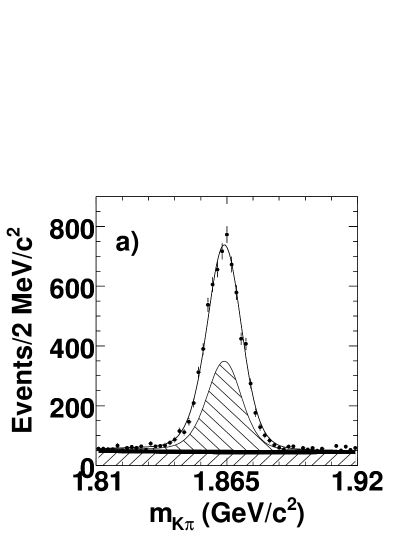
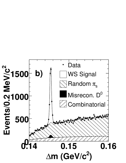
Figure 1: a) $m_{K\pi}$ for wrong-sign (WS) candidates with $0.1445<\Delta m<0.1465{\mathrm{\,Ge\kern-1.00006ptV\!/}c^{2}}$, and b) $\Delta m$ for WS candidates with $1.843<m_{K\pi}<1.883{\mathrm{\,Ge\kern-1.00006ptV\!/}c^{2}}$. The fitted PDFs are overlaid.

The measured proper-time distribution for the RS signal is described by an exponential function convolved with a resolution function whose parameters are determined by the fit to the data. The resolution function is the sum of three Gaussians with widths proportional to the estimated event-by-event proper-time uncertainty $\sigma_{t}$. The random $\pi_{\rm s}^{+}$ background is described by the same proper-time distribution as signal events, since the slow pion has little weight in the vertex fit. The proper-time distribution of the combinatorial background is described by a sum of two Gaussians, one of which has a power-law tail to account for a small long-lived component. The combinatorial background and real $D^{0}$ decays have different $\sigma_{t}$ distributions, as determined from data using a background-subtraction technique based on the fit to $m_{K\pi}$ and $\Delta m$.

The fit to the RS proper-time distribution is performed over all events in the full $m_{K\pi}$ and $\Delta m$ region. The PDFs for signal and background in $m_{K\pi}$ and $\Delta m$ are used in the proper-time fit with all parameters fixed to their previously determined values. The fitted $D^{0}$ lifetime is found to be consistent with the world-average lifetime PDG2006 .

The measured proper-time distribution for the WS signal is modeled by Eq. (7) convolved with the resolution function determined in the RS proper-time fit. The random $\pi_{\rm s}^{+}$ and misreconstructed $D^{0}$ backgrounds are described by the RS signal proper-time distribution since they are real $D^{0}$ decays. The proper-time distribution for WS data is shown in Fig. 2. The fit results with and without mixing are shown as the overlaid curves.

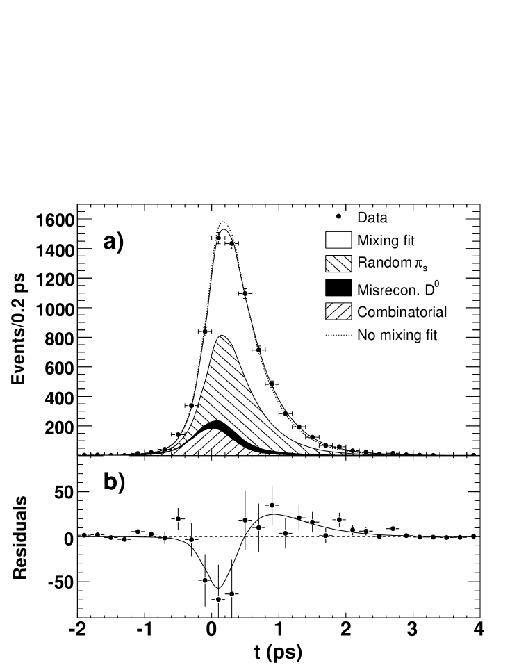
Figure 2: a) Projections of the proper-time distribution of combined $D^{0}$ and $\kern 1.99997pt\overline{\kern-1.99997ptD}{}^{0}$ WS candidates and fit result integrated over the signal region $1.843<m_{K\pi}<1.883{\mathrm{\,Ge\kern-1.00006ptV\!/}c^{2}}$ and $0.1445<\Delta m<0.1465{\mathrm{\,Ge\kern-1.00006ptV\!/}c^{2}}$. The result of the fit allowing (not allowing) mixing but not $C\!P$ violation is overlaid as a solid (dashed) curve. b) The points represent the difference between the data and the no-mixing fit. The solid curve shows the difference between fits with and without mixing.

The fit with mixing provides a substantially better description of the data than the fit with no mixing. The significance of the mixing signal is evaluated based on the change in negative log likelihood with respect to the minimum. Figure 3 shows confidence-level (CL) contours calculated from the change in log likelihood ($-2\Delta\ln{\cal L}$) in two dimensions (${x^{\prime}}^{2}$ and $y^{\prime}$) with systematic uncertainties included. The likelihood maximum is at the unphysical value of ${x^{\prime}}^{2}=-2.2\times 10^{-4}$ and $y^{\prime}=9.7\times 10^{-3}$. The value of $-2\Delta\ln{\cal L}$ at the most likely point in the physically allowed region (${x^{\prime}}^{2}=0$ and $y^{\prime}=6.4\times 10^{-3}$) is $0.7$ units. The value of $-2\Delta\ln{\cal L}$ for no-mixing is $23.9$ units. Including the systematic uncertainties, this corresponds to a significance equivalent to 3.9 standard deviations ($1-\mbox{CL}=1\times 10^{-4}$) and thus constitutes evidence for mixing. The fitted values of the mixing parameters and $R_{\rm D}$ are listed in Table III. The correlation coefficient between the ${x^{\prime}}^{2}$ and $y^{\prime}$ parameters is $-0.94$.

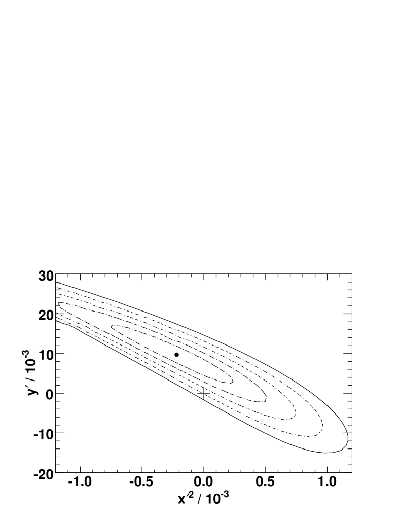
Figure 3: The central value (point) and confidence-level (CL) contours for $1-\mbox{CL}=0.317\ (1\sigma)$, $4.55\times 10^{-2}\ (2\sigma)$, $2.70\times 10^{-3}\ (3\sigma)$, $6.33\times 10^{-5}\ (4\sigma)$ and $5.73\times 10^{-7}\ (5\sigma)$, calculated from the change in the value of $-2\ln{\cal L}$ compared with its value at the minimum. Systematic uncertainties are included. The no-mixing point is shown as a plus sign ($+$).

Table 1: Results from the different fits. The first uncertainty listed is statistical and the second systematic.

Fit type	Parameter	Fit Results ($/10^{-3}$)
No $C\!P$ viol. or mixing	$R_{\rm D}$	$3.53$ $\pm$	$0.08$ $\pm$	$0.04$
No $C\!P$ violation	$R_{\rm D}$	$3.03$ $\pm$	$0.16$ $\pm$	$0.10$
	${x^{\prime}}^{2}$	$-0.22$ $\pm$	$0.30$ $\pm$	$0.21$
	$y^{\prime}$	$9.7$ $\pm$	$4.4$ $\pm$	$3.1$
$C\!P$ violation allowed	$R_{\rm D}$	$3.03$ $\pm$	$0.16$ $\pm$	$0.10$
	$A_{\rm D}$	$-21$ $\pm$	$52$ $\pm$	$15$
	${x^{\prime}}^{2+}$	$-0.24$ $\pm$	$0.43$ $\pm$	$0.30$
	$y^{\prime+}$	$9.8$ $\pm$	$6.4$ $\pm$	$4.5$
	${x^{\prime}}^{2-}$	$-0.20$ $\pm$	$0.41$ $\pm$	$0.29$
	$y^{\prime-}$	$9.6$ $\pm$	$6.1$ $\pm$	$4.3$

Allowing for the possibility of $C\!P$ violation, we calculate the values of $R_{\rm D}=\sqrt{R_{\rm D}^{+}R_{\rm D}^{-}}$ and $A_{\rm D}=(R_{\rm D}^{+}-R_{\rm D}^{-})/(R_{\rm D}^{+}+R_{\rm D}^{-})$ listed in Table III, from the fitted $R_{\rm D}^{\pm}$ values. The best fit points $({x^{\prime}}^{2\pm},y^{\prime\pm})$ shown in Table III are more than three standard deviations away from the no-mixing hypothesis. The shapes of the $({x^{\prime}}^{2\pm},y^{\prime\pm})$ CL contours are similar to those shown in Fig. 3. All cross checks indicate that the close agreement between the separate $D^{0}$ and $\kern 1.79997pt\overline{\kern-1.79997ptD}{}^{0}$ fit results is coincidental.

As a cross-check of the mixing signal, we perform independent $\{m_{K\pi},\,\Delta m\}$ fits with no shared parameters for intervals in proper time selected to have approximately equal numbers of RS candidates. The fitted WS branching fractions are shown in Fig. 4 and are seen to increase with time. The slope is consistent with the measured mixing parameters and inconsistent with the no-mixing hypothesis.

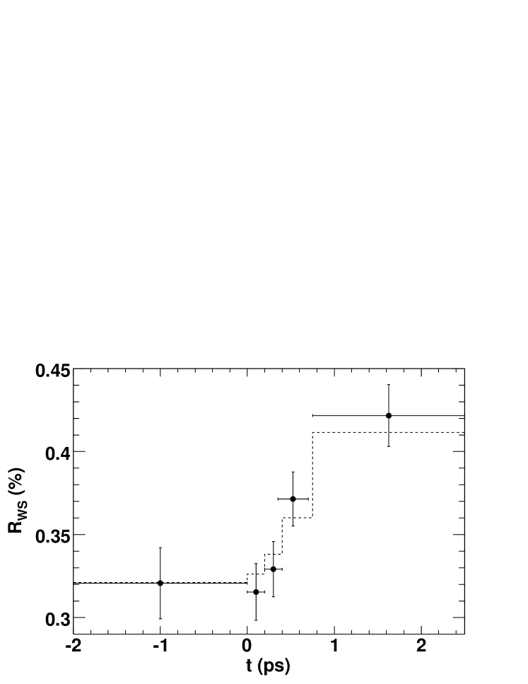
Figure 4: The WS branching fractions from independent $\{m_{K\pi},\,\Delta m\}$ fits to slices in measured proper time (points). The dashed line shows the expected wrong-sign rate as determined from the mixing fit shown in Fig. 2. The $\chi^{2}$ with respect to expectation from the mixing fit is 1.5; for the no-mixing hypothesis (a constant WS rate), the $\chi^{2}$ is 24.0.

We validated the fitting procedure on simulated data samples using both MC samples with the full detector simulation and large parametrized MC samples. In all cases we found the fit to be unbiased. As a further cross-check, we performed a fit to the RS data proper-time distribution allowing for mixing in the signal component; the fitted values of the mixing parameters are consistent with no mixing.

In evaluating systematic uncertainties in $R_{\rm D}$ and the mixing parameters we considered variations in the fit model and in the selection criteria. We also considered alternative forms of the $m_{K\pi}$, $\Delta m$, proper time, and $\sigma_{t}$ PDFs. We varied the $t$ and $\sigma_{t}$ requirements. In addition, we considered variations that keep or reject all $D^{*+}$ candidates sharing tracks with other candidates.

For each source of systematic error, we compute the significance ${s}_{i}^{2}=2t\big{[}\ln{\cal L}({x^{\prime}}^{2},\,y^{\prime})-\ln{\cal L}({x^{\prime}}^{2}_{i},y^{\prime}_{i})\big{]}/2.3$, where $({x^{\prime}}^{2},\,y^{\prime})$ are the parameters obtained from the standard fit, $({x^{\prime}}^{2}_{i},y^{\prime}_{i})$ the parameters from the fit including the $i^{th}$ systematic variation, and ${\cal L}$ the likelihood of the standard fit. The factor 2.3 is the 68% confidence level for 2 degrees of freedom. To estimate the significance of our results in $({x^{\prime}}^{2},\,y^{\prime})$, we reduce $-2\Delta\ln{\cal L}$ by a factor of $1+\mathchar 28934\relax s_{i}^{2}=1.3$ to account for systematic errors. The largest contribution to this factor, $0.06$, is due to uncertainty in modeling the long decay time component from other $D$ decays in the signal region. The second largest component, $0.05$, is due to the presence of a non-zero mean in the proper time signal resolution PDF. The mean value is determined in the RS proper time fit to be $3.6\rm\,fs$ and is due to small misalignments in the detector. The error of $15\times 10^{-3}$ on $A_{\rm D}$ is primarily due to uncertainties in modeling the differences between $K^{+}$ and $K^{-}$ absorption in the detector.

In conclusion we summarize the BABAR  evidence for $D^{0}$-$\kern 1.79997pt\overline{\kern-1.79997ptD}{}^{0}$ mixing. Our result is inconsistent with the no-mixing hypothesis at a significance of 3.9 standard deviations. We measure $y^{\prime}=[9.7\pm 4.4\hbox{ (stat.)}\pm 3.1\hbox{ (syst.)}]\times 10^{-3}$, while ${x^{\prime}}^{2}$ is consistent with zero. We find no evidence for $C\!P$ violation and measure $R_{\rm D}$ to be $[0.303\pm 0.016\hbox{ (stat.)}\pm 0.010\hbox{ (syst.)}]\%$. The result is consistent with Standard Model estimates for mixing.

References

- (1) B. Aubert et al. (BABAR Collaboration), SLAC-PUB-12494.
- (2) B. Aubert et al. (BABAR Collaboration), Phys. Rev. Lett. 91, 121806 (2003).
- (3) M. Staric, et al., Phys. Rev. Lett. 98, 211803 (2007).
- (4) B. Aubert et al. (BABAR Collaboration), Phys. Rev. Lett. 97, 221803 (2006).
- (5) D.M. Asner et al. Phys. Rev. D72, 012001 (2005).
- (6) L.M. Zhang, arXiv 0704, 1000v2 [hep-ex], submitted to Phys. Rev. Lett.
- (7) B. Aubert et al. (BABAR Collaboration), Phys. Rev. Lett. 98, 211802 (2007).
- (8) The use of charge-conjugate modes is implied unless otherwise noted.
- (9) W.-M. Yao et al. (Particle Data Group), J. Phys. G33 1 (2006).