Crustal structure below Popocatépetl Volcano (Mexico) from analysis of Rayleigh waves.

Abstract

An array of ten broadband stations was installed on the Popocatépetl volcano (Mexico) for five months between October 2002 and February 2003. 26 regional and teleseismic earthquakes were selected and filtered in the frequency time domain to extract the fundamental mode of the Rayleigh wave. The average dispersion curve was obtained in two steps. Firstly, phase velocities were measured in the period range [2 - 50] s from the phase difference between pairs of stations, using Wiener filtering. Secondly, the average dispersion curve was calculated by combining observations from all events in order to reduce diffraction effects. The inversion of the mean phase velocity yielded a crustal model for the volcano which is consistent with previous models of the Mexican Volcanic Belt. The overall crustal structure beneath Popocatépetl is therefore not different from the surrounding area and the velocities in the lower crust are confirmed to be relatively low. Lateral variations of the structure were also investigated by dividing the network into four parts and by applying the same procedure to each sub-array. No well defined anomalies appeared for the two sub-arrays for which it was possible to measure a dispersion curve. However, dispersion curves associated with individual events reveal important diffraction for 6 s to 12 s periods which could correspond to strong lateral variations at 5 to 10 km depth.

, , , and

1 Introduction

Popocatépetl is a large andesitic strato-volcano, located 60 km south-east of Mexico City and 40 km West of Puebla (fig. 1.a). It belongs to the Trans-Mexican Volcanic Belt (MVB). Its large cone is the second highest summit of Mexico (5452 m above sea level) with an elipsoidal 600-800 m wide crater.
The present active period began on December 21st 1994. Since 1996, an andesitic to dacitic dome cyclicly grows into the crater and bursts producing high plumes of gas and ash (Arcieniega-Ceballos et al., 2000; Wright et al., 2002). More than 100 000 persons could potentially be directly affected by an eruption and ashes could affect an area with more than 20 million people (De La Cruz-Reyna and Siebe, 1997; Macías and Siebe, 2005).
The overall crustal structure beneath the MVB is relatively well studied (Campillo et al., 1996; Valdes et al., 1986; Shapiro et al., 1997). On the contrary, the crustal seismic structure beneath Popocatepetl is not well known. Receiver functions analysis by Cruz-Atienza et al. (2001), using 4 events from South America, indicates that a Low Velocity Zone may be present beneath a station located 5 km north of the crater.
The aim of this paper is to improve the knowledge of this complex volcano structure, and particularly to determine if the whole crust beneath the volcano is significantly different from the rest of the MVB. The first kilometers of crust beneath several volcanoes have been studied (e.s. Dawson et al., 1999; Laigle et al., 2000; Benz et al., 1996). Typical volcanic anomalies are low velocity zones, attributed to the presence of partial melt, or high velocity zones, due to solidified magmatic intrusions.
We concentrate on the S-wave structure, as S-wave velocities are very sensitive to temperature changes and to the presence of even small amounts of partial melt. The easiest way to get an overall picture of S-wave velocities is through surface wave analysis. However, the traditional 2-stations methods can not be used in this rather diffractive environnement as measurements would possibly be strongly biased due to local and regional diffraction (Wielandt, 1993; Friederich et al., 1995). An alternative approach is therefore to use array analysis. Such methods have been used on volcanoes, particularly for tremor source location (Métaxian et al., 2002; Almendros et al., 2002) or for shallow structure study (See for example Saccorotti et al., 2001). More details can be found in Chouet (2003) who presents a state of the art on volcano seismology.
The dispersion curve had to be measured over a wide frequency range (0.02-1 Hz) to study the overall crustal structure beneath Popocatépetl. The array configuration which was strongly influenced by topography and logistic issues was such that we could not use spatial Fourier transforms outside a very narrow frequency range. Consequently methods based on wavenumber decomposition were excluded. The use of time-domain methods was problematic as we needed a good frequency resolution.
These considerations led us to use the procedure of Pedersen et al. (2003) to measure phase velocities across the array. The assumption behind this method is that the records are constituted by one single plane wave which propagates through the array. Even though this hypothesis is most probably wrong for most individual events, it may be corrected by averaging out unwanted waves (diffraction effects, non plane waves, etc) using events from different directions. The variability between different events will also provide an error estimate on the dispersion curve. To increase frequency range and azimuthal coverage we used both teleseismic and local events.
After a short description of the data and the processing methods used, we present and discuss the main results, with a comparison of the overall crustal structure beneath the volcano to that of the MVB.

2 Data

An array of nine stations (Guralp CMG 40T) with three-components broadband sensors (30-60 s cut-off period) was installed in October 2002 on the Popocatépetl volcano and continuously recorded four months of seismic events. Figure 1.b shows the array geometry. The station altitudes were between 2500 and 4300 m above sea level. The reference altitude used in this study corresponds to an average level of 3500 m a.s.l.
To obtain dispersion curves in a period range of 2 to 50 s, we chose to use both teleseimic and local events with epicentral distances between 200 and 15000 km (see fig. 2). We selected vertical components of events with a good signal to noise ratio and with well developed Rayleigh waves. The usuable frequency range for the two types of events overlapped, however the long period part of the dispersion curve was mainly calculated using teleseismic events while the shorter periods were dominated by regional events.
Prior to the array analysis, we deconvolved the data with the instrument responses. The second step of this analysis was to enhance the signal-to-noise ratio through time-frequency filtering (Levshin et al., 1989). In this part of the analysis we firstly applied multiple filter to the data and identified the group velocity dispersion curve by the maximum amplitude at each frequency. We secondly integrated this curve to obtain the phase velocities and subtracted the corresponding phase $\theta(f)$ at each frequency to obtain a non dispersive signal. A time window was then applied onto the non-dispersive wave to suppress noise and the phase $\theta(f)$ was finally added. Fig. 3 shows the comparison between an unfiltered record (3.a), with its corresponding group velocity (3.c), and filtered record (3.b) of a teleseismic event.
The time-frequency filter efficiently reduces the influence of noise, body waves and higher mode Rayleigh waves. It also makes it possible to identify and exclude events whose fundamental mode of Rayleigh waves is not well separated from other waves. 10 events were rejected during this stage. A further 12 events were excluded during the array analysis, leaving 26 events. Table 1 contains the final event list, and figure 2 shows their distribution. The number of teleseismic events was too small to ensure a correct back-azimuth distribution, but there were events from all quadrants. The regional events were mainly located in the Pacific Coast subduction and the Caribbean Islands, ensuring a back-azimuth range between N126^o (South East) to N273^o (West).

3 Methodology

To measure phase velocities, we follow Pedersen et al. (2003). In this method, the phase velocity at a given frequency is obtained in two steps. Firstly, each event is analysed independently. In this step, the phase $\phi$ of the Wiener filtering $W(f)$ is transformed into time delays $\Delta t$ between each pair of stations using $\Delta t=\phi/(2\pi f)$. The Wiener filtering in the frequency domain that we use is given by:

$$W(f)=\frac{S_{XY}\ast Han(f)e^{j2\pi ft_{0}}}{\sqrt{S_{XX}\ast Han(f)}\sqrt{S_{YY}\ast Han(f)}}$$

$S_{XX}$, $S_{YY}$ and $S_{XY}$ are respectively the Fourier transforms of the autocorrelations and intercorrelation of the two signals , $Han(f)$ is the Fourier transform of the Hanning fonction $han(t)$ and $t_{0}$ is the delay of the intercorrelation peak. $\ast$ represents the convolution product. A grid-search on velocity and back-azimuth is applied to find the best fitting plane wave that would explain the observed time delays. The fit is calculated with the L1 norm, i.e the average absolute difference between observed and predicted time delays. The knowledge of the back-azimuth makes it possible to subsequently calculate the distance between each pair of stations projected onto the slowness vector. In this way each event yields a series of (distance,delay) points.
Secondly, a bootstrap process is applied (Schorlemmer et al., 2003; Efron and Tibshirani, 1996): 500 bootstrap samples are created by resampling the 26 events of the data set. For each bootstrap sample, the phase velocity is calculated as the inverse of the slope of the best fitting line through all the (distance, delay) points. The L1 norm is also used here to estimate the fit between observations and predictions. The points are associated with weighting which reflects how well the data fitted the assumption of a plane wave in the first step of the analysis. The final phase velocity and the associated uncertainity are obtained as the average and standard deviation over the 500 samples.
The advantages of this method are 1) stabilization of delay measurements through Wiener filtering; 2) stabilization of back-azimuths and phase velocities through the use of the L1 norm; 3) weighting of the events in the final phase velocity calculation according to the quality of the back-azimuth estimate; 4) estimation of realistic error bars on the final dispersion curve. For more details, we refer to Pedersen et al. (2003).
The last part of this analysis consists in inverting the dispersion curves. We used the two-step inversion methods proposed by Shapiro et al. (1997). Firstly, the average dispersion curve was inverted using a linearized, classical dispersion scheme (Herrmann, 1987) to find a simple shear wave model which fitted the dispersion curve. We then used this model for a stochastic nonlinear Monte-Carlo inversion. Interface depths and shear-wave velocities were randomly changed into a new model which was kept and used in the next iteration if it fitted the dispersion curve within the error bars. This second step was repeated 5000 times. We eliminated unrealistic models by applying loose constraints on Moho depth (between 40 and 50 km depth) and on the S-wave velocity near the surface in agreement to the existing models (between 1.5 and 3 km/s). We finally calculated the average model and we verified that the corresponding dispersion curve fitted within the error bars of the observed one. The error bars of the final models were computed as the standard deviation of all the acceptable models. Quality factors and P-wave velocities were kept constant during the inversion as their influence was significantly smaller than the error bars of the dispersion curve.

4 Results

To detect differences between the crust under the Popocatépetl and the standard crust of the MVB, one can compare the equivalent shear wave velocities profiles. As surface wave inversions are non-unique it is however useful to also compare the dispersion curves which correspond to the existing models.
The models that we compare with were from: 1) Cruz-Atienza et al. (2001) who obtained their model through inversion of receiver functions using four teleseismic events from South America at station PPIG (located 5 km north of the Popocatépetl crater, see fig.1); 2) Campillo et al. (1996) who inversed the group velocities of local events between the Guerrero Coast and Mexico City; 3) Valdes et al. (1986) whose model is the result of a seismic refraction study in Oaxaca. We recalculated the phase velocities corresponding to these models. Shapiro et al. (1997) detected lateral variations of uppermost crustal structure within the MVB using surface wave group velocities. Due to the limited depth penetration in their study (10 km), their models are not included in our figures, but will be integrated in the discussion of the results.

4.1 Full array

We firstly used all the stations and the 26 events to measure the ’overall dispersion curve’, i.e. the average dispersion curve within the full array. The phase velocities were unstable above 35 s period and were not used in the inversions.
In Figure 4.a we compare our dispersion curve with the ones corresponding to the earth model derived by Campillo et al. (1996), Cruz-Atienza et al. (2001) and Valdes et al. (1986). For periods longer than 8 s, the Campillo et al. (1996) curve is similar to ours. For short periods, the velocities increase rapidly with period, similarly to the Cruz-Atienza et al. (2001) curve.
We verified that our inversions of the observed phase velocities were independent of which of the three reference models (see fig 4.b) was used as starting model. The results shown here are obtained by using the one of Campillo et al. (1996) as it has the advantage of fitting our data well and it only has four layers. The latter is important to allow for an efficient exploration of the parameter space in the Monte Carlo inversion.
Our preferred model (fig. 4.b) shows low shear velocities (2.2 km/s) between the surface and 3 km depth, overlying a layer with velocities increasing slowly from 3.4 to 3.7 km/s between 6 to 20 km depth. The transition between the two layers may be either a strong gradient or a sharp interface. The lower part of the crust has a constant velocity of 3.75 km/s down to Moho which is located at 45 km depth. The velocity below Moho is approximatively 4.3 km/s. The lower crust and upper mantle velocity as well as the Moho depth are not well resolved due to trade-off between these parameters and because of a maximal period of 35s.
The boundary depths that we obtained are however consistent with existing models, in particular with Campillo et al. (1996). Our near surface velocities are however significantly lower and our upper crustal velocities slightly higher than those of Campillo et al. (1996), while the two models are virtually almost identical in the lower crust. The low velocity of the surface layer is relatively well constrained, however we can not exclude that the layer would be slightly thinner with slightly lower velocity. This layer, also identified by Cruz-Atienza et al. (2001), can be associated with the poorly consolidated materials of the volcano cone. Shapiro et al. (1997) find that the velocities in the upper 2 km are low beneath the southern part of the MVB where the volcanic activity is recent as compared to the northern part. Our results imply that the overall crustal structure below Popocatépetl is not significantly different from that of the MVB.
We verified whether an 6-layers initial model with a Low velocity zone between 6 and 10 km inspired by the Cruz-Atienza et al. (2001) model, would yield a significantly different result. The resulting model is not different from our prefered model (fig 4.b), in particular there is no significant Low Velocity Zone. We do not see any indication that the Low Velocity Zone observed by Cruz-Atienza et al. (2001) is a general feature of the volcano.

4.2 Sub-arrays

To investigate lateral variations within the area, we divided the array into sub-arrays for which we calculated dispersion curves independently. The use of sub-arrays was particularly difficult as these arrays were composed of only three stations, so technical problems at any of the relevant stations would render the analysis impossible. It was possible to measure dispersion curves for the Southern (South sub-array: FPC, FPP, FPX) and the western sub-array (West sub-array: FPA, FPP, FPX). The dispersion curves for these two sub-arrays are shown in figure 5. At the largest period the analysis is mainly based on teleseismic events, out of which only 3 or 4 events were avalaible for the sub-array analysis. The phase velocity error bars are consequently large at long period ($>$ 25 s for the South sub-array and $>$ 15 s for the West sub-array).
The dispersion curves for the South sub-array ( located around the active crater) and the West sub-array was respectively measured with 13 and 14 events (see table 1). For the West sub-array, individual dispersion curves show strong oscillations between 6 and 12 s, particularly for events coming from the South or the East. These oscillations, probably due to local diffraction result in large error bar for the final dispersion curve. However, the dispersion curves beneath the two sub-arrays are not significantly different from the overall dispersion curve.
The phase velocities obtained with events for which the surface waves propagated through the volcano before encountering the array are more fluctuating than those obtained with other events. As the majority of the events are located South and South-West of the array, the individual dispersion curves are more fluctuant with the period at the North and East sub-arrays (composed of stations FPA, FPP, FMI and FPC) than for the other sub-arrays. It was consequently not possible to calculate a stable dispersion curve for these two arrays.
The starting model for the inversion for the sub-arrays South and West is the model found with the full array, approximated by four layers. The estimated velocities are not significantly different from those of the overall model. Nevertheless, for the South array velocities are slightly smaller between 6 and 10 km depth, and the surface velocities are higher. The differences are however smaller than the error bars of the overall model.

5 Discussion and Conclusion

The average crust beneath the Popocatépetl volcano appears to be similar to the MVB crust. There is therefore no indication of large scale crustal anomalies associated with Popocatépetl as compared to the MVB. We do however confirm that the lower crust in the area is likely to be associated with relatively low shear wave velocities (3.75 km/s). Close to the surface, the velocity is approximatively 2.2 km/s over at least a depth of 3 km. It probably corresponds to the poorly consolidated material of the cone (such as volcanic slags and ash and pyroclastic deposits) overlying the 2 km-thick volcanic layer of the MVB crust (Shapiro et al., 1997).
We speculate that the oscillations observed for the sub-arrays between 6 and 12 s periods is associated with diffraction by lateral heterogeneity at 5-10 km depth as this period range corresponds to wavelengths between 16 and 36 km. To obtain strong diffraction, the heterogeneity must be of considerable size (i.e. of the order of the wavelength), as surface waves are not strongly diffracted by many small heterogeneities (Chammas et al., 2003). However, the lack of Low Velocity Zone turns down the hypothesis of a large continuous magma chamber. We speculate that either the interface located at 4 km depth in the average model fluctuate strongly, or that an abrupt lateral change takes place immediately beneath the central part of the volcano. The unresolved velocities at 5-10s period at the West and South sub-arrays indicate that future arrays should be designed so as to give good constraints at 5-10 km depth. To obtain this, more stations and a larger recording period are necessary.
More seismic events with a better azimutal distribution would improve the smoothing and the error bars of the dispersion curves and make it possible to include receiver function analysis and coupled Rayleigh-Love inversion.

TABLE AND FIGURE CAPTIONS

Table 1: Origine time, epicentre distance and back-azimuth of the events used for measuring the dispersion curves for the full array or with the sub-arrays (columns 5 and 6).

Figure 1: (a) Location of the Popocatépetl volcano and (b) array geometry used in the analysis. PPIG is a permanent station used by Cruz-Atienza et al. (2001) and is not used in this study.

Figure 2: Location and azimuth distribution of (a) teleseismic and (b) local events used in the array analysis.

Figure 3: Example of frequency-time filtering: a) Trace recorded at FPX, of the event at 03:37:42 GMT on november 03th 2002; b) Same trace after filtering; c) Group velocity of this event before filtering.

Figure 4: a: Comparison of dispersion curves:
1) Uncertainities of our observed dispersion curves ($\pm$ 1 standard deviation, grey area) for the full array and 2) dispersion curve calculating with our average model (solid line); 3) Dispersion curve for Valdes et al. (1986); 4) Same for Campillo et al. (1996); 5) Same for Cruz-Atienza et al. (2001).
Fig. 4. b: Comparison of crustal models:
1) Error bars ($\pm$ 1 standard deviation, grey area) and 2) average S-wave velocity model (solid line); 3) Crustal model for Valdes et al. (1986); 4) Same for Campillo et al. (1996); 5) Same for Cruz-Atienza et al. (2001).

Figure 5: Dispersion curves of the full array (dotted line) and the two sub-arrays (solid line) with their uncertainities (grey area): a) South sub-array; b) West sub-array. In insert: sub-array geometry and back-azimuths of the events used.

date	hour	epicentre	back-	West	South
		(km)	azimuth	array	array
2002/11/03	03:37:42	11021	316
2002/11/04	03:19:18	14875	79		X
2002/11/04	10:00:47	342	240	X	X
2002/11/04	13:57:32	366	241	X	X
2002/11/05	14:05:07	650	273	X	X
2002/11/06	16:02:37	279	186	X	X
2002/11/06	16:24:17	321	192	X	X
2002/11/06	18:04:05	390	234	X	X
2002/11/07	15:14:06	7834	319	X	X
2002/11/08	23:20:41	301	168	X	X
2002/11/09	00:14:18	980	126	X	X
2002/11/09	06:05:58	7779	164
2002/11/15	19:58:31	10135	150
2002/11/20	22:59:14	383	233	X	X
2002/11/21	02:53:14	1903	111	X	X
2002/11/26	00:48:15	7337	319
2002/11/26	16:30:59	379	236	X	X
2002/11/27	01:35:06	6511	323	X
2002/12/01	02:27:55	10444	234	X
2002/12/14	01:37:48	304	234
2002/12/21	08:01:31	276	189
2003/01/21	02:46:47	1024	125
2003/01/22	19:41:38	607	268
2003/01/22	20:15:34	618	267
2003/01/31	15:56:52	275	216
2003/02/19	03:32:36	6749	321

Table 1:

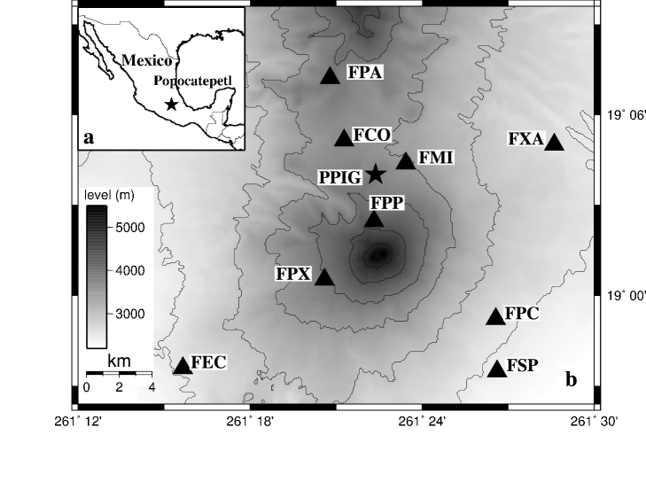
Figure 1:

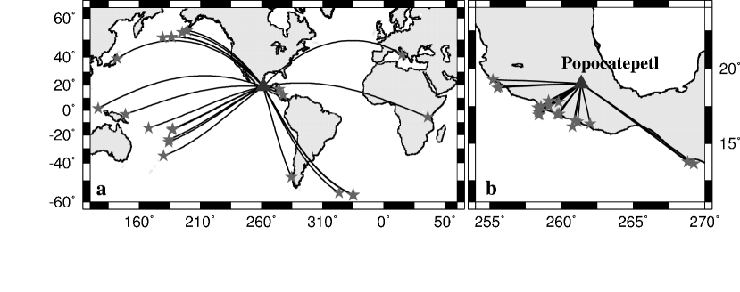
Figure 2:

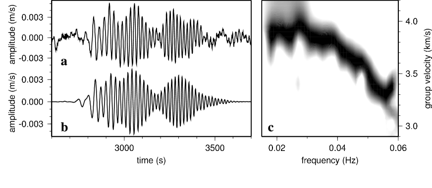
Figure 3:

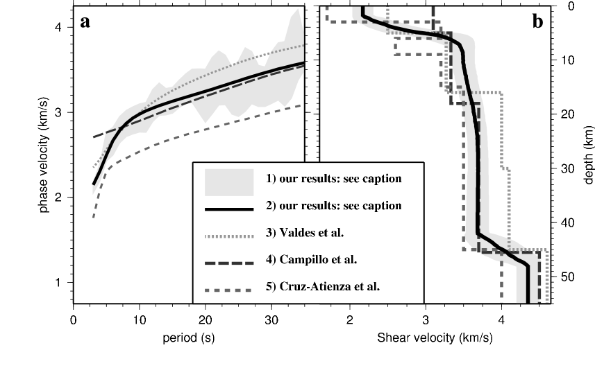
Figure 4:

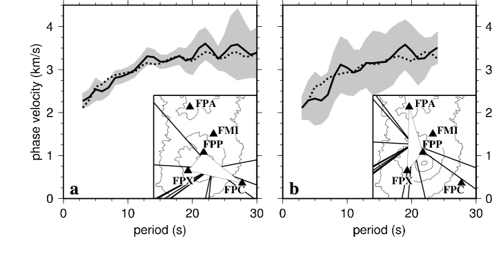
Figure 5:

References

- Almendros et al. (2002) Almendros, J., Chouet, B., Dawson, B., Huber, C., 2002. Mapping the sources of the seismic wave field at Kilauea Volcano, Hawaï, using data recorded on multiple seismic antenna. Bull. Seism. Soc. Am. 92, 2333-2351.
- Arcieniega-Ceballos et al. (2000) Arcieniega-Ceballos, A., Chouet, B.A., Dawson, P., 2000. Very long-period signals associated with vulcanian explosions at Popocatépetl Volcano, central Mexico. J. Volcanol. Geotherm. Res. 26, 3013-3016.
- Benz et al. (1996) Benz, H.M., Chouet, B.A., Dawson, P.B, Lahr, J.C., Page, R.A., Hole, J.A., 1996. Three-dimensional P and S wave velocity structure of Redoudt volcano, Alaska. J. Geophys. Res. 101(B4), 8111-8128.
- Campillo et al. (1996) Campillo, M., Singh, S.K., Shapiro, N., Pacheco, J., Herrmann, R.B., 1996. Crustal structure South of the Mexican Volcanic belt, based on group velocity dispersion. Geofísica Internacional 35, 361-370.
- Chammas et al. (2003) Chammas, R., Abraham, O., Cote, P., Pedersen, H. A., Semblat, J. F., 2003. Characterization of Heterogeneous Soils Using Surface Waves: Homogenization and Numerical Modeling, International Journal of Geomechanics 3, 55-63.
- Cruz-Atienza et al. (2001) Cruz-Atienza, V.M., Pacheco, J.F., Singh, S.K., Shapiro, N.M., Valdes C., Iglesias, A., 2001. Size of Popocatépetl volcano explosions (1997-2001) from waveform inversion. Geophys. Res. Lett. 28, 4027-4030.
- Chouet (2003) Chouet, B., 2003. Volcano Seimology. Pure and Applied Geophysics 160, 739-788.
- Dawson et al. (1999) Dawson, P.B., Chouet, B.A., Okubo, P.G., Villasenor, A., Benz, H.M., 1999. Three-dimensional velocity structure of the Kilauea caldera, Hawaii. Geophys. Res. Lett. 26, 2805-2808.
- De La Cruz-Reyna and Siebe (1997) De La Cruz-Reyna, S., Siebe, C., 1997. The giant Popocatépetl stirs. Nature 388, 227.
- Efron and Tibshirani (1996) Efron, B. and Tibshirani, R., 1986. Bootstrap methods for standard errors, confidence intervals and other measurements of statistical accuracy. Statistical Science 1, 54-77.
- Friederich et al. (1995) Friederich, W., Wielandt, E., 1995. Interpretation of seismic surface waves in regional networks: joint estimation of wavefield geometry and local phase velocity. Method and numerical tests. Geophys. J. Int. 120, 731-744.
- Herrmann (1987) Herrmann, R.B., 1987. Computers programms in seismology, Volume IV: Surface waves. Saint Louis University, Missouri.
- Laigle et al. (2000) Laigle, M., Hirn, A., Sapin, M., Lépine, J.C., Diaz, J., Gallart, J., Nicolich, R., 2000. Mount Etna dense array local earthquake P and S tomography and implications for volcanic plumbing. J. Geophys. Res. 105(B9), 21633-21646.
- Levshin et al. (1989) Levshin, A.L., Yanovskaia, T.B., Lander, A.V., Bukchin, B.G., Barmin, M.P., Ratnikova, L.I. and Its, E.N., 1989. Surface waves in a vertically inhomogeneous media. In: Keilis-Borok, V.I. (Ed.), Seismic Surface Waves in a Laterally Inhomogeneous Earth. Kluwer, Dordrecht, pp. 131-182.
- Macías and Siebe (2005) Macías, J.L., Siebe, C., 2005. Popocatépetl crater filled to the brim: significance for hazard evaluation. J. Volcanol. Geotherm. Res. 141, 327-330.
- Métaxian et al. (2002) Métaxian, J.-P., Lesage, P., Valette, B., 2002. Locating sources of volcanic tremor and emergent events by seismic triangulation: Application to Arenal volcano, Costa Rica. J. Geophys. Res. 107(B10), 2243-2261.
- Pedersen et al. (2003) Pedersen, H.A., Coutant, O., Deschamps, A., Soulage, M., Cotte, N., 2003. Measuring surface wave phase velocities beneath small broad-band arrays: tests of an improved algorithm and application to the French Alps. Geophys. J. Int. 154, 903-912.
- Saccorotti et al. (2001) Saccorotti G., Almendros J., Carmona E., Ibánez J.M., Del Pezzo E., 2001, Slowness Anomalies from two dense seismic arrays at Deception Island volcano, Antartica. Bull. Seism. Soc. Am. 91, 561-571.
- Schorlemmer et al. (2003) Schorlemmer, D., Neri, G., Wiemer, S., Mostaccio, A., 2003. Stability and significance tests for b-value anomalies: Example from the Tyrrhenian Sea. Geophys. Res. Lett. 30(16), 1835-1841.
- Shapiro et al. (1997) Shapiro, N.M., Campillo, M.,Paul, A., Singh, S.K., Jongmans, D., Sanchez-Sesma, F.J., 1997. Surface wave propagation across the Mexican Volcanic Belt and the origin of the long period seismic wave amplification in the valley of Mexico. Geophys. J. Int. 128, 151-166.
- Valdes et al. (1986) Valdes, C.M., Mooney, W.D., Singh, S.K.,Meyer, R.P., Lomnitz, C., Luetgert, J. H., Hesley, B.T., Lewis, B.T.R., Mena, M., 1986. Crustal structure of Oaxaca, Mexico from seismic refraction measurements. Bull. Seism. Soc. Am. 76, 547-564.
- Wielandt (1993) Wielandt, E., 1993. Propagation and structural interpretation of nonplane waves. Geophys. J. Int. 113, 45-53.
- Wright et al. (2002) Wright, R., De La Cruz-Reyna, S., Harris, A., Flynn, L., Gomez-Palacios, J.J., 2002. Infrared satellite monitoring at Popocatépetl: Explosions, exhalations, and cycle of dome Growth. J. Geophys. Res. 107(B8), 1029-1045.