A Galaxy in Transition: Structure, Globular Clusters, and Distance of the
Star-Forming S0 Galaxy NGC 1533 in Dorado

Abstract

We use two-band imaging data from the Advanced Camera for Surveys on board the Hubble Space Telescope for a detailed study of NGC 1533, an SB0 galaxy in the Dorado group surrounded by a ring of H i. NGC 1533 appears to be completing a transition from late to early type: it is red, but not quite dead. Faint spiral structure becomes visible following galaxy subtraction, and luminous blue stars can be seen in isolated areas of the disk. Dust is visible in the color map in the region around the bar, and there is a linear color gradient throughout the disk. We determine an accurate distance from the surface brightness fluctuations (SBF) method, finding $(m{-}M)=31.44\pm 0.12$ mag, or $d=19.4\pm 1.1$ Mpc. We then study the globular cluster (GC) colors, sizes, and luminosity function (GCLF). Estimates of the distance from the median of the GC half-light radii and from the peak of the GCLF both agree well with the SBF distance. The GC specific frequency is $S_{N}=1.3\pm 0.2$, typical for an early-type disk galaxy. The color distribution is bimodal, as commonly observed for bright galaxies. There is a suggestion of the redder GCs having smaller sizes, but the trend is not significant. The sizes do increase significantly with galactocentric radius, in a manner more similar to the Milky Way GC system than to those in Virgo. This difference may be an effect of the steeper density gradients in loose groups as compared to galaxy clusters. Additional studies of early-type galaxies in low density regions can help determine if this is indeed a general environmental trend.

1. Introduction

The Hubble Space Telescope (HST) has opened the door to our understanding of extragalactic star cluster systems, revealing numerous globular clusters (GCs) in early-type galaxies (e.g. Gebhardt & Kissler-Patig, 1999; Peng et al. 2006) as well as “super-star clusters” (SSCs) in late-type galaxies (Larsen & Richtler 2000), especially starbursts (e.g. Meurer et al. 1995, Maoz et al. 1996). In early-type systems the color distribution of the GCs is often bimodal, consisting of a blue metal-poor component and a red metal-rich component (e.g. West et al. 2004; Peng et al. 2006). This observation gives a hint to the connection between the early- and late-type systems. Mergers often have particularly strong starbursts and rich populations of SSCs, as seen for example in NGC4038/39 - “the Antennae” system (Whitmore & Schweizer 1995; Whitmore et al. 1999), and hierarchical merging is one possible origin for the redder population of GCs in early-type galaxies (e.g., Ashman & Zepf 1998; Beasley et al. 2002; Kravtsov & Gnedin 2005).

Much of the research on GC systems has concentrated on galaxy clusters which are rich in early-type galaxies (e.g., the ACS Virgo Cluster Survey, Côté et al. 2004; the ACS Fornax Cluster Survey, Jordán et al. 2007). Early-type galaxies in groups and the field are somewhat less studied, particularly with HST and the Wide Field Channel (WFC) of its Advanced Camera for Surveys (ACS). The relatively wide ($3\farcm 4$) field of view of the ACS WFC combined with its fine pixel sampling make it an exceptional tool for imaging GCs out to a few tens of Mpc where they have measurable angular sizes (Jordán et al. 2005).

Here we report HST ACS/WFC imaging of the SB0 (barred lenticular) galaxy NGC 1533 in the Dorado group. This group is in the “Fornax wall” (Kilborn et al. 2005) and hence at a similar distance to the Fornax cluster (e.g., Tonry et al. 2001). Dorado is interesting in that it is richer than the Local Group but still dominated by disk galaxies (its brightest members being the spiral NGC 1566 and the S0 NGC 1553), and its members have H i masses similar to non-interacting galaxies with the same morphology (Kilborn et al. 2005). While the apparent crossing time of the group is only $\sim 13$% of the age of the universe (Firth et al. 2006; see also Ferguson & Sandage 1990), the most recent analyses conclude the group is unvirialized (Kilborn et al. 2005; Firth et al. 2006), which may explain the richness in spirals and H i.

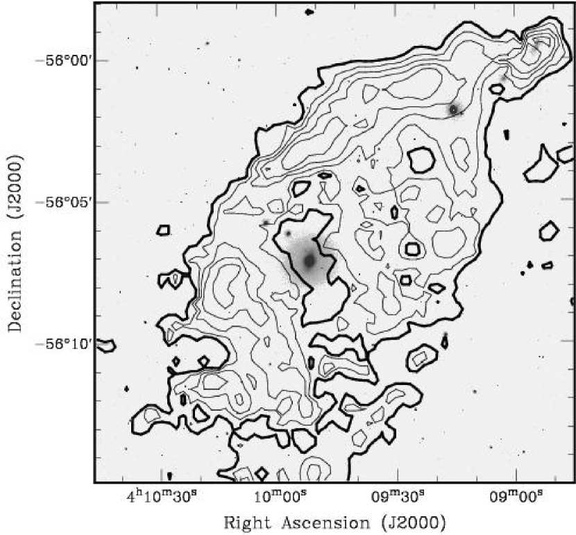
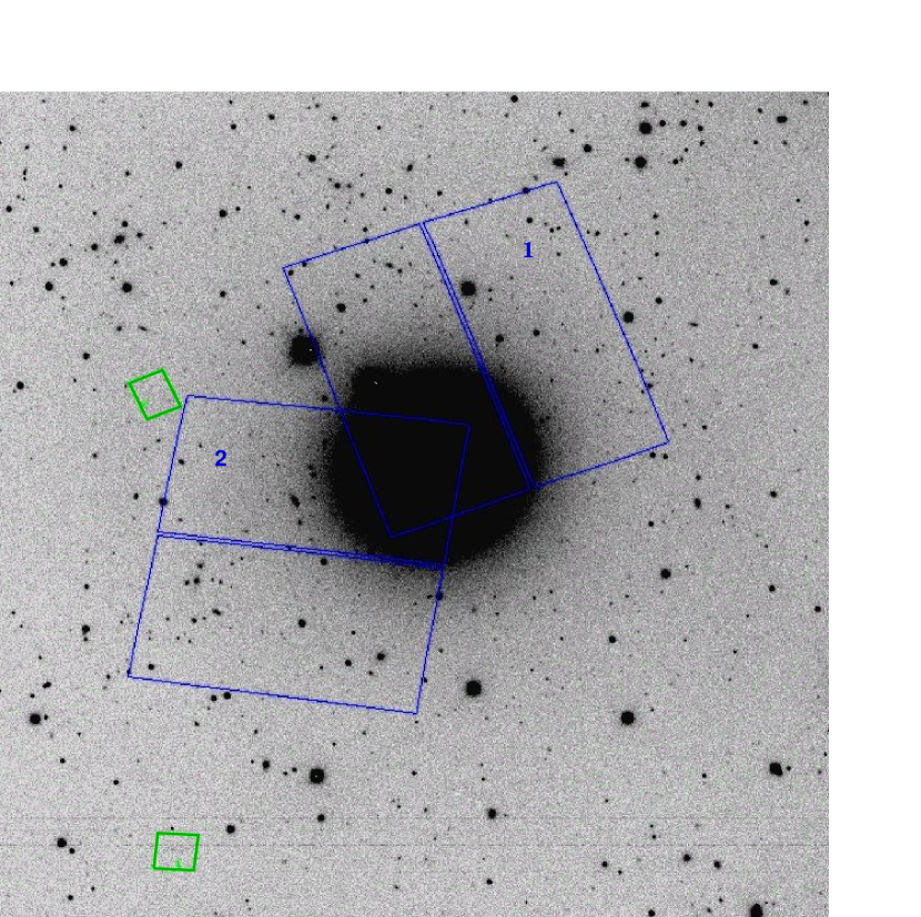
Figure 1.— Left panel: H i contours from Ryan-Weber et al. (2003) are overlaid on a ground-based $R$-band image of the NGC 1533 field from the SINGG survey (Meurer et al. 2006). The outermost contour (bold) is at a column density of $10^{20}$ cm^-2, and the contours increase in steps of $0.5{\times}10^{20}$ cm^-2. The small companion galaxies IC 2038/2039 are in the upper right corner of the image. NGC 1533 itself is in an H i “hole” (the galaxy center is not detected), and this distribution has been described as a ring. Right panel: ACS HRC (green) and WFC (blue) fields of view for the two HST roll angles described in the text (labeled 1 and 2). The outlines of the camera fields are overlaid on a $\sim\,$9′ portion of the SINGG $R$-band image. North is up and East is to the left in both panels.

NGC 1533 is the seventh brightest member of the Dorado group, with $M_{V}{\,\approx\,}{-}20.7$. It lies within the virial radius, but is a $\sim\,$2-$\sigma$ velocity outlier (Kilborn et al., 2005; Firth et al. 2006) so that it is moving at high speed through the intra-group medium. A vast H i arc is seen in the outskirts of NGC 1533 connected to the Sdm galaxy IC 2038 and the small S0 galaxy IC 2039 (Ryan-Weber et al. 2004). This suggests that NGC 1533 is “stealing” ISM from its companions or has cannibalized another gas-rich satellite (see Figure 1, left panel). As is typically seen in S0 galaxies, star formation is weak in NGC 1533. Observations of this galaxy in spectroscopic surveys note the presence of emission lines (Jorgensen et al. 1997; Bernardi et al. 2002); the nuclear spectrum available from the 6dF survey (Jones et al. 2005) shows [N ii]6584 and weak H$\alpha$. H$\alpha$ imaging from the Survey of Ionization in Neutral Gas Galaxies (SINGG, an H$\alpha$ imaging survey of H i selected galaxies; Meurer et al. 2006) shows a few weak H ii regions beyond the end of its bar (the nucleus is too bright to allow faint nuclear H ii regions to be detected in the SINGG images), as well as a scattering of very faint “intergalactic H ii regions”. These are discussed in more detail by Ryan-Weber et al. (2004) who show that they are so faint that it would only take one to a few O stars to ionize each one. Although its current rate is low, the star formation in NGC 1533 illustrates another possible channel for building up cluster systems in early-type galaxies: slow re-ignited star formation in ISM stripped from companions.

The ACS WFC images of NGC 1533 used in the present study were obtained with HST as “internal parallel images” while the ACS High Resolution Channel (HRC) was pointed at the intergalactic H ii regions (HST GO Program 10438; M. Putman, PI). The HRC observations are discussed elsewhere (Werk et al. 2007, in preparation). Here we use the WFC observations to measure the structural properties of the galaxy, characterize its GC population, and use the GC luminosity function (GCLF), GC half-light radii, and surface brightness fluctuations (SBF) to provide accurate distance estimates. The contrast between NGC 1533, a (weakly) star-forming gas-rich barred S0 in a loose group environment, and galaxies in the richer environments of the Virgo and Fornax cluster, provides a useful test of the ubiquity of the various relations found in the denser environments.

The following section describes the observations and data reductions in more detail. Sec. 3 discusses the galaxy morphology, structure, color profile, and isophotal parameters. Sec. 4 presents the SBF analysis and galaxy distance, while Sec. 5–7 discuss the GC colors, effective radii, luminosity function, and specific frequency. The final section summarizes our conclusions.

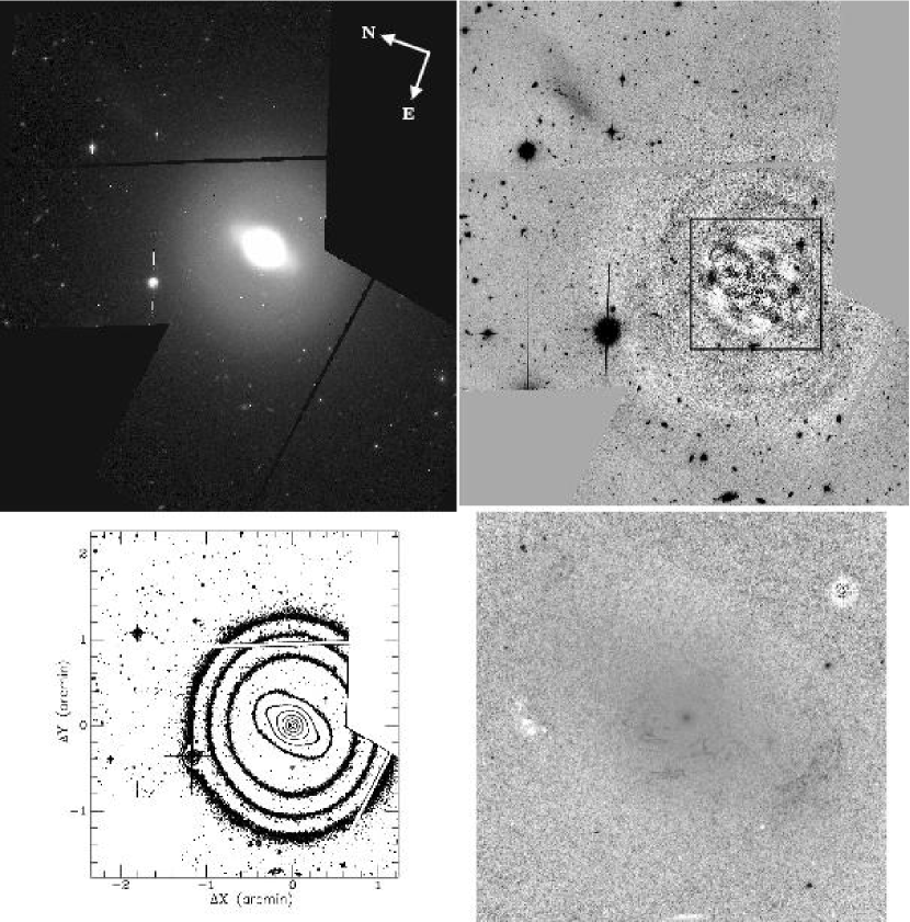
Figure 2.— Upper left: Combined F814W ACS/WFC image of NGC 1533. Lower left: Contour map of a 3$\farcm$6$\times$4$\farcm$0 portion of the image. Contours are plotted in steps of a factor of two in intensity, with the faintest being at $\mu_{I}=20.7$ mag arcsec^-2. Upper right: The image following galaxy model subtraction, showing the faint spiral structure (the “plume” 2′ north of the galaxy is a ghost image). The same 3$\farcm$6$\times$4$\farcm$0 field is shown; the box marks the central 1′. Lower right: Colormap of the central 1′ region of NGC1533, with dark indicating red areas and white indicating blue. The dark spot at center marks the center of the galaxy. Dust can be seen as faint, dark, wispy features. A compact blue star-forming region is visible to the left of the galaxy center, near the center-left of the map.

2. Observations and Data Reduction

As noted above, during the primary ACS HRC observations of H II regions in the halo of NGC 1533, the WFC was used for parallel imaging of the main galaxy. These observations were carried out on 2005 September 25 with HST V3-axis position angle PA_V3 = 110$\fdg$15 and on 2005 November 18 with PA_V3 = 170$\fdg$75; we refer to these throughout as “roll 1” and “roll 2,” respectively. Figure 1 shows the positions and orientations of the primary ACS/HRC fields, and the overlapping parallel ACS/WFC fields, at the two roll angles.

2.1. Image Processing

NGC 1533 was imaged in the F814W and F606W bandpasses of the ACS/WFC. Eight exposures totaling 4950 s in F814W, and four exposures totalling 1144 s in F606W, were taken at each of the two roll angles. Following standard calibration by the STScI archive, the data were processed with the ACS IDT “Apsis” pipeline (Blakeslee et al. 2003) to produce final, geometrically corrected, cleaned images with units of accumulated electrons per pixel. Apsis also ensures the different bandpass images are aligned to better than 0.1 pix and performs automatic astrometric recalibration of the processed images.

We calibrated the photometry using the Vega-based $m_{1}$ zero points from Sirianni et al. (2005): $m_{1,\,F606}=26.398$ and $m_{1,\,F814}=25.501$. Galactic extinction was taken into account using the dust maps of Schlegel et al. (1998) and the extinction ratios from Sirianni et al. (2005). We determined extinction corrections of $A_{606}=0.045$ mag and $A_{814}=0.029$ mag for the F606W and F814W bandpasses, respectively. For comparison to other studies, we also converted the measured (F606W$\,-\,$F814W) colors to Johnson–Cousins $(V{-}I)$ using the empirically-based prescription given by Sirianni et al.

We processed the data at the two roll angles with Apsis both separately and combined together. The upper left panel of Figure 2 shows the result from the combined processing, which is useful for analyzing the galaxy 2-D surface brightness distribution and isophotal parameters using the largest angular range. However, for the SBF and globular cluster analyses, we considered each pointing separately and then merged the results at the end. This was done to avoid PSF and orientation mismatch effects (e.g., diffraction spikes and effects due to the gate structure of the CCDs do not match up when combining images with differing orientations). For each filter image at each pointing, we modeled the galaxy light using the “elliprof” software written by J. Tonry for the SBF Survey of Galaxy Distances (Tonry et al. 1997) and described in more detail by Jordán et al. (2004). Saturated areas, bright sources, diffraction spikes, and dusty regions were masked out for a better model fit. The galaxy model was then subtracted from the image, revealing faint sources and residual features, including faint spiral structure as discussed in Sec. 3.

2.2. Object Photometry

Object detection was performed with SExtractor (Bertin & Arnout 1996) using the galaxy-subtracted image for detection and an RMS image for the weighting. The RMS image gives the uncertainty per pixel including the effects of instrumental and photon shot noise, as well as the additional “noise” from the galaxy surface brightness fluctuations. It is constructed as described in detail by Jordán et al. (2004):

$${\rm RMS}\,=\,\sqrt{({\rm RMS}_{Ap})^{2}+(K_{F}\ast model)}\,,$$ (1)

where ${\rm RMS}_{Ap}$ is the Apsis RMS image based on the instrumental and shot noise alone (Blakeslee et al. 2003), model is the galaxy surface brightness model, and $K_{F}$ gives the ratio of the variance per pixel from SBF, $\sigma^{2}_{L}$, to that from photon shot noise from the galaxy, $\sigma^{2}_{p}$. The $K_{F}$ factor depends on the bandpass, exposure time, galaxy distance (which determines the apparent amplitude of the SBF), and the image resolution; it can be estimated as

$$K_{F}\;=\;\frac{\sigma^{2}_{L}}{\sigma^{2}_{p}}\;=\;\frac{1}{p}\,10^{-0.4(\overline{m}_{F}-m^{\ast}_{1,F})}\,,$$ (2)

where $m^{\ast}_{1,F}=m_{1,F}+2.5\,\log(T)$, $T$ is the total exposure time, $\overline{m}_{F}$ is the SBF magnitude in the given bandpass, and $p$ is a factor that reduces the SBF variance because of the smoothing effect of the PSF. We adopt $\overline{m}_{F814}\approx 30$ for NGC 1533 based on the measurement from Tonry et al. (2001) in the very similar $I_{C}$ bandpass (and confirmed by our SBF result in Sec 4) and assume $\overline{M}_{F606}-\overline{M}_{F814}$ $\approx 2$ based on expectations from stellar population models (Liu et al. 2000; Blakeslee et al. 2001) to determine $\overline{m}_{F606}$. Following Jordán et al. (2004), we convolved simulated noise images with the ACS PSFs to determine the $p$ factor in Eq. 2; thus, we reduced the variance ratio by 12 for F606W and by 13 for F814W and finally determined the values $K_{F606}=1.1$ and $K_{F814}=6.0$.

We ran SExtractor in “dual image mode,” such that object detection, centroiding, and aperture determination was performed only in the deeper F814W image, while the object photometry was performed in both the F606W and F814W images. This ensures that the same pixels are used for the photometry in both images (see Benítez et al. 2004 for a detailed discussion). The catalogs produced by SExtractor include magnitudes measured within various fixed and automatic apertures. By comparing color measurements of the same objects at the two different roll angles, we chose to use the colors measured within an aperture of radius 4 pixels. Since we are mainly interested here in compact, only marginally resolved, globular cluster candidates, we applied a uniform correction of 0.016 mag to the colors measured in this aperture, based on the difference in the F606W and F814W aperture corrections (Sirianni et al. 2005). These colors were transformed to $(V{-}I)$ following Sirianni et al., as described above. For the total $I$-band magnitude, we use the extinction-corrected, aperture-corrected Vega-based F814W magnitude $I_{814}$. According to Sirianni et al., for objects with $(V{-}I)\approx 1$, this should differ from Cousins $I_{C}$ by $\lesssim\,$0.006 mag, or less than the expected zero-point error of $\sim\,$0.01 mag.

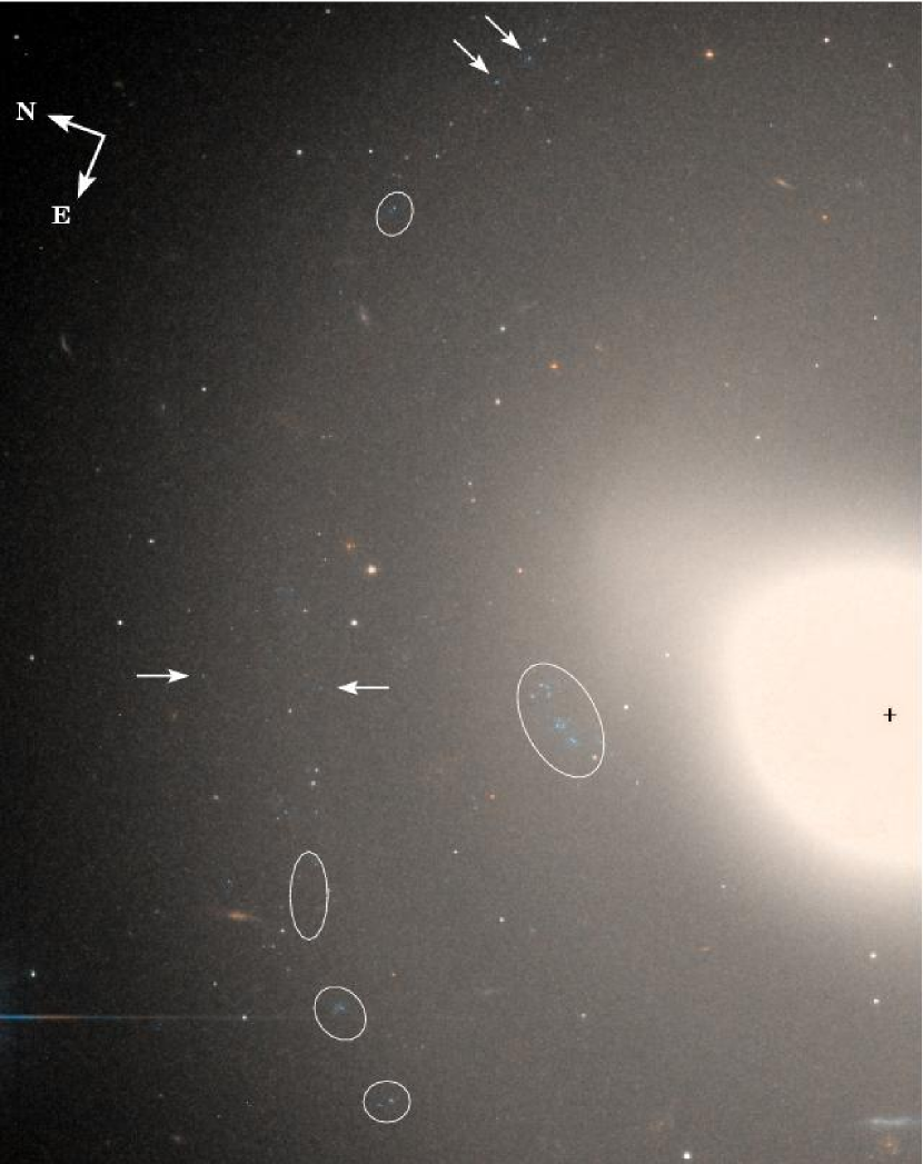
Figure 3.— Blue objects in a $1\farcm 1{\times}1\farcm 4$ region in NGC 1533. The ellipses mark the known H II regions from Meurer et al. (2006), and the arrows point out individual, compact blue objects which appear to be in the same faint spiral arm. The two white sources within the largest H ii region are GC candidates. The galaxy center is marked and the orientation is the same as in Fig. 2.

3. Galaxy Properties

Tonry et al. (2001) reported SBF distances to six members of the Dorado group. However, one of these (NGC 1596) was found to be about 20% closer than the others; omitting it gives a mean distance modulus for Dorado of $\langle m{-}M\rangle=31.40\pm 0.09$ mag, or $\langle d\rangle=19.1\pm 0.8$ Mpc. (We have revised the published numbers downward by 3%, as noted in Sec. 4 below, before taking the average.) NGC 1533 itself had a poorly determined ground-based SBF distance of $d=20.8\pm 4.0$, the largest among the Dorado galaxies, but in agreement with the mean distance given the large uncertainty. Based on 24 Dorado group members, Kilborn et al. (2005) report a mean velocity of $1250\pm 57$ km s^-1, with $\sigma=282$ km s^-1. NGC 1533’s velocity is 790 km s^-1, indicating a motion through the group of 460 km s^-1 towards us.

3.1. Morphology

The morphological type of NGC 1533 in the RC3 is $T=-3$ (de Vaucouleurs et al. 1991), indicating an early-type S0. Buta et al. (2006) classify it as (RL)SB0⁰, meaning that it is a barred, intermediate-type S0 containing both an inner lens structure and a ring-like feature in the disk. In a morphological study of 15 early-type disk galaxies, Laurikainen et al. (2006) give an inner radius of 44″ for the ring. Some of these features are evident in the contour map in Figure 2: the round central bulge and convex-lens shape of its surrounding isophotes, the oblong bar, and the disk are all visible. In addition, the model-subtracted image in the upper right panel reveals spiral features that are difficult to see in the original image. The faint spiral arms appear to emanate from the ends of the bar and wrap around by 360^∘. Sandage & Brucato (1979) also noted a “suggestion of weak spiral pattern in outer lens (or disk)” in NGC 1533. It seems likely that this is the “ring” seen by Buta et al. (2006) and Laurikainen et al. (2006). Thus, NGC 1533 appears to be in the late stages of transition from a barred spiral to a barred S0 galaxy. Such morphological transitions are believed to underlie the observed evolution in the cluster morphology-density relation at intermediate redshift (e.g., Dressler et al. 1997; Postman et al. 2005). Understanding the processes involved in similar transitions at low redshift can therefore guide our understanding of cluster evolution.

The subtracted image also shows luminous material about 2$\farcm$0 to the north/northwest of the NGC 1533 galaxy center, beyond the galaxy disk. This feature is only visible in the F814W image, not in the F606W or ground-based images. It is apparently an internal camera reflection from a bright star outside the field of view.

The color map in the lower right panel of Fig. 2 reveals the presence of wispy dust (darker areas in the color map) to the east and south of the nucleus within the central 20″ along the bar. Moreover, a compact region of bluer light is visible at the center left edge of the color map, about 23″ to the northeast of the galaxy nucleus. This position coincides with the brightest H ii region seen in the H$\alpha$ image of Meurer et al. (2006). Our F606W image shows the individual blue stars, as well as diffuse emission around them in this and the other H ii regions. The diffuse light probably arises from the emission lines (especially H$\alpha$, [O iii]) in the F606W passband. The areas of dust and star formation support the view of NGC 1533 as a galaxy recently converted from spiral to S0. However, it should be noted that dust features are found in roughly half of bright early-type galaxies when studied at high resolution (Ferrarese et al. 2006), and isolated star formation is not too uncommon.

At larger radius within the disk (outside the color map in the figure), we find several other small groups, or isolated examples, of unresolved blue objects with colors $(V{-}I)\approx 0$ and magnitudes $I_{814}\gtrsim 23.5$. Some of these are visible in Figure 3, and the ones associated with H ii regions are marked in the color-magnitude diagram presented in Sec. 5. They may be a mix of post-asymptotic giant branch (PAGB) stars, indicating an intermediate age population, and small isolated regions of star formation. Several of the blue objects, highlighted in Figure 3, are spread out along one of the spiral arms. The likely connection with the spiral arm in this case points towards these being a small, dispersed group of fairly young stars.

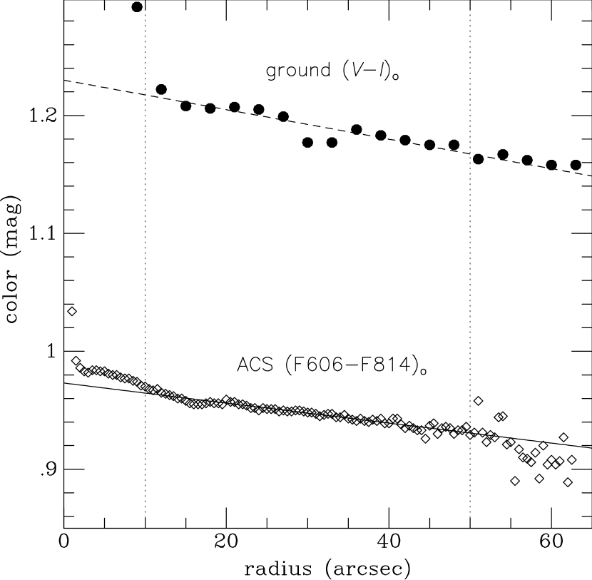
Figure 4.— Surface brightnesses in 0$\farcs$5 circular rings for the Vega-calibrated F606W and F814W bandpasses are plotted as a function of $r^{{1}/{4}}$ (left). The dashed and solid lines show linear fits to the data inside a radius of 16″ where the bulge dominates. The lower and upper dotted lines show the sky levels in F606W and F814W, respectively. NGC 1533 colors from the ground-based $(V{-}I)$ data (solid circles) of Tonry et al. (1997) and our ACS (F606W$\,-\,$F814W) imaging (open diamonds) is shown as a function of radius (right). The lines show linear fits to the data points in the radial range $10\arcsec<r<50\arcsec$.

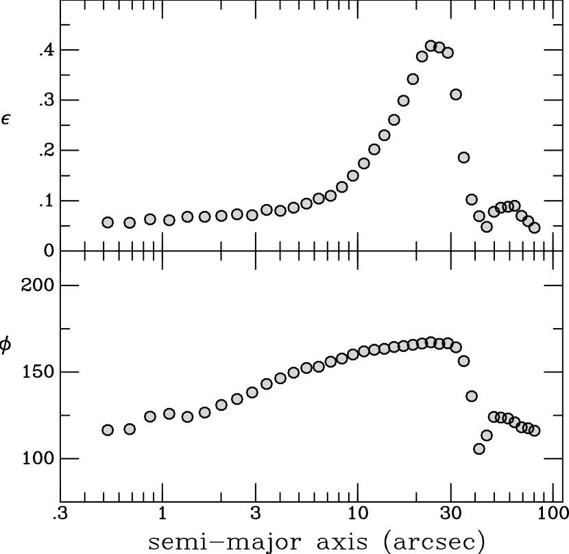
Figure 5.— Isophotal parameters for NGC 1533. Ellipticity $\epsilon$ and position angle $\phi$ from the galaxy isophote modeling are shown versus the semi-major axis of the isophote (left). The higher-order $A_{3}$ and $A_{4}$ harmonic terms, measuring deviations of the isophotes from pure ellipses, are shown versus the isophotal semi-major axis (left). The peak in the $A_{4}$ profile occurs at 21″, whereas the peak in $\epsilon$ occurs at 24″.

3.2. Galaxy Surface Photometry and Structure

Although NGC 1533 has a complex isophotal structure, it can also be enlightening to study the simple one-dimensional light profile. Figure 4 (left panel) shows the galaxy surface brightness profiles in F606W and F814W. Within a radius of about 16″, the profile is reasonably well fit by a de Vaucouleurs $r^{1/4}$-law profile (a straight line in the figure). Between 16″ and $\sim\,$45″, the profile becomes much flatter; this includes the inner disk and area around the bar. In the outer disk, beyond $\sim\,$50″, the profile steepens again.

The right panel of Figure 4 shows the galaxy color profile. In addition to our measured (F606W$\,-\,$F814W) profile, we show the ground-based $(V{-}I)$ photometry for this galaxy from the Tonry et al. (1997) study (which provides median and average surface photometry measured in 3″ radial bins, without removal of external sources). The ground-based data come from multiple long exposures with the Cerro Tololo 4 m Blanco telescope at a pixel scale of 0$\farcs$47 pix^-1. They suffer from poor seeing (1$\farcs$5 in $I$, 1$\farcs$8 in $V$) and severe central saturation; however, the systematic error on the color is only 0.018 mag (Tonry et al. 2001). Similar gradients are observed in both sets of photometry. By binning the data at the same scales and comparing colors over a radial range of 10″ – 50″, we determined:

$$(V{-}I)\,=\,(1.196\pm 0.003)+(1.2\pm 0.2)\,[{(\hbox{F606W}-\hbox{F814W})}-0.95]\,,$$ (3)

with an RMS scatter of 0.010 mag in the fit. This relation yields $(V{-}I)$ colors between the empirical (based on stellar photometry) and theoretical (based on synthetic spectra and the bandpass transmission curves) transformations provided by Sirianni et al. (2005), which differ between themselves by $\sim\,$0.07 mag in this color range. It is in better agreement with the empirical transformation, differing by about 0.02 mag, as compared to $\sim\,$0.05 mag with the synthetic transformation, which is probably more uncertain because the F606W bandpass differs substantially from standard $V$. Likewise, Brown et al. (2005) reported that when transformations were calculated based on the bandpass definitions, empirical corrections of order $\sim\,$0.05 mag were required to match globular cluster data from $(V{-}I)$ to (F606W$\,-\,$F814W). In any case, Eq. 3 allows for a precise matching of our measured (F606W$\,-\,$F814W) colors to Johnson–Cousins $(V{-}I)$ over the small range of the galaxy color gradient. This is important for calibrating our SBF measurements in Sec. 4 below.

We also performed parametric 2-D surface photometry fits with Galfit (Peng et al. 2002). For the simplest case, we used a double Sérsic (1968) model to fit the bulge and disk (the bar was poorly modeled, mostly as part of the bulge component). This analysis yielded a bulge-to-total ratio $B/T=0.42$, with half-light radii of 7″ and 46″ for the bulge and disk, respectively. The Sérsic index for the bulge was $n=2.0$, intermediate between an exponential and a de Vaucouleurs profile. However, the fit gave $n=0.4$ for the disk, or a profile that goes as $\sim\exp(-\alpha r^{2.5})$, which is even more spatially truncated than a Gaussian. This agrees with what was seen in the 1-D plot, where the profile remains fairly constant over a large radial range then drops off more steeply beyond about 50″. We also made fits with 3 and 4 components. These gave better model residuals, but the different components did not neatly break down into clearly distinct physical components such as bulge, bar, disk, halo (or lens, etc.), so the interpretation was unclear.

3.3. Isophotal Parameters

Figure 5 presents the radial profiles of the isophotal ellipticity, position angle, and $A_{3}$ and $A_{4}$ harmonic parameters. The upper left panel of the figure shows that the galaxy is quite round within 10″ (bulge) and beyond 40″ (disk). However, it reaches a maximum ellipticity $\epsilon=0.41$ at a semi-major axis distance of 24″, corresponding to the semi-major axis of the bar. As seen in the lower left panel, there is also a gradual isophotal twist from $PA\approx 125^{\circ}$ near a radius of 1″, to $PA\approx 170^{\circ}$ where the ellipticity reaches its maximum. Laurikainen et al. (2006) found similar ellipticity and orientation trends for NGC 1533 from their analysis of ground-based $K$-band data, although they do not appear to have resolved the structure inside a few arcseconds.

The right panels of Figure 5 show the amplitudes of the third-order and fourth-order harmonic terms, which measure the deviations of the isophotes from pure ellipses (Jedrzejewski 1987). The values reported by elliprof are the relative amplitudes of these higher order harmonics with respect to the mean isophotal intensity, i.e., $A_{3}=I_{3}/I_{0}$ and $A_{4}=I_{4}/I_{0}$. The upper right panel of the figure shows that the galaxy remains quite symmetric at all radii, since the $A_{3}$ component remains near zero. However, the $A_{4}$ component, an indicator of “diskiness,” reaches a maximum of 13% at a major axis of 21″, then drops suddenly. Thus, $A_{4}$ reaches its maximum at a smaller radius than does the ellipticity, since the major axis of the lens-like isophotes is smaller than that of the bar. This agrees with the contour map in Figure 2, where the “convex lens” shape appears embedded within the oblong bar.

4. Surface Brightness Fluctuations Distance

We measured the SBF amplitude in four radial annuli for each of the two F814W observations at the different roll angles. We used the software and followed the standard analysis described by Tonry et al. (1997), Ajhar et al. (1997), Jensen et al. (1998), Blakeslee et al. (1999, 2001), and references therein. More details on the SBF analysis for ACS/WFC data are given by Mei et al. (2005) and Cantiello et al. (2005, 2007). Briefly, after subtracting the galaxy model as described above, we fitted the large-scale spatial residuals to a two-dimensional grid (we used the SExtractor sky map for this) and subtracted them to produce a very flat “residual image.” All objects above a signal-to-noise threshold of 10 were removed (masked) from the image. We used this high threshold to avoid removing the fluctuations themselves, or the brightest giants in the galaxy. As described in the following sections, with the resolution of HST/ACS we are able to detect and remove globular clusters (the main source of contamination) to more than a magnitude beyond the peak of the GCLF, and the residual contamination is negligible. We also used the F606W image and the color map to identify and mask the dusty regions and small areas of star formation.

We then modeled the image power spectra in the usual way, using the template WFC F814W PSF provided by the ACS IDT (Sirianni et al. 2005) and a white noise component. We performed the analysis in four radial annuli: $64<R_{p}\leq 128$, $128<R_{p}\leq 256$, $256<R_{p}\leq 512$, and $512<R_{p}\leq 840$, where $R_{p}$ is the projected radius in pixels. The annuli grow by factors of two in order to preserve the same approximate signal level in each; the outermost limit is set by the proximity of the galaxy to the edge of the ACS image.

The SBF amplitude is the ratio of the galaxy image variance (normalization of the PSF component of the power spectrum) to the surface brightness; it has units of flux, and is usually converted to a magnitude called $\overline{m}$. The absolute $I$-band SBF magnitude has been carefully calibrated according to the galaxy $(V{-}I)$ color (Tonry et al. 1997, 2000). With a 0.06 mag adjustment to the zero point (Blakeslee et al. 2002) as a consequence of the final revisions in the HST $H_{0}$ Key Project Cepheid distances (Freedman et al. 2001), the calibration is

$$\overline{M}_{I}\;=\;-1.68{\pm}0.08\,+\,(4.5\pm 0.25)[(V{-}I)_{0}-1.15]\,.$$ (4)

For objects with colors similar to the GCs or the mean galaxy surface brightness, we have assumed $I_{814}=I_{C}$, since both the empirical and synthetic transformations from Sirianni et al. (2005) agree in predicting that the difference should be $<\,$0.01 mag. However, the SBF is much redder, with a typical color $\overline{M}_{V}{-}\overline{M}_{I}\approx 2.4$ mag (Blakeslee et al. 2001). This is outside the color range of the empirical transformation, but the synthetic one gives $\overline{M}_{I}=\overline{M}_{814}+0.04$, with an estimated uncertainty of $\sim\,$0.02 mag. We apply this correction and tabulate our SBF results in Table 1 for the four annuli at the two different roll angles. The table also gives the galaxy color converted to $(V{-}I)$ using Eq. 3 in the same annuli and with the same masking as used for the SBF analysis, and the resulting distance moduli determined from Eq. 4.

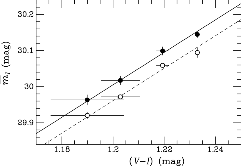
Figure 6.— SBF measurements in four radial annuli in NGC 1533 from the roll 1 (filled circles) and roll 2 (open circles) observations. The solid and dashed lines have slopes of 4.5, as given by the published $\overline{m}_{I}$–$(V{-}I)$ calibration, and are fitted only in the zero point. Although internally quite consistent, the two sets of observations give distance moduli that differ by 0.04 mag.

Figure 6 provides a graphical representation the SBF results. The measurements at the two different roll angles are remarkably consistent, except for a systematic offset of 0.04 mag. Weighted averages of the annuli give mean distance moduli and formal errors of $31.456\pm 0.008$ and $31.416\pm 0.009$ mag for rolls 1 and 2, respectively. The galaxy appears at very different locations in the field of view for the two observations, in fact on different CCD chips. We verified that the difference in the photometry itself was negligible (about ten times smaller than the $(m{-}M)$ offset). However, the ACS/WFC does have some spatial variation in the PSF (Krist 2003), and temporal variations can be caused by jitter, sun angle, etc. Any mismatch in the PSF template used for the power spectrum analysis directly affects the SBF measurement, and this is the most likely cause of the small difference.

We therefore average the results from the two roll angles and use the 0.04 mag difference as a more realistic estimate of the measurement uncertainty. To this, we add uncertainties of 0.01 mag in the absolute calibration of F814W, 0.02 mag for the transformation of $\overline{m}$ to the standard $I$ band, $4.5\times 0.018=0.08$ mag from the systematic uncertainty in the $(V{-}I)$ color used for the calibration (Sec. 3.2), and 0.08 mag from the $\overline{M}_{I}$ calibration zero point. Finally, we obtain $(m{-}M)=31.44\pm 0.12$ mag, or $d=19.4\pm 1.1$ Mpc. This is an improvement by a factor of 3.5 compared to the ground-based distance from Tonry et al. (2001), and agrees well with the mean SBF result for the Dorado group (see Sec. 3 above). Thus, although NGC 1533 is something of a velocity outlier, its distance is the same as the group mean. Our measurement translates to a spatial scale of 94.0 pc per arcsec, or 4.70 pc per ACS/WFC pixel, which we adopt for the globular cluster analysis in the following sections.

5. Globular Cluster Colors

To obtain a sample of globular cluster candidates from the object photometry described in Sec. 2.2 above, we selected objects with $19<I_{814}<24$ mag, $0.5\leq(V{-}I)\leq 1.5$, FWHM $\leq$ 4 pix (0$\farcs$2) in each bandpass, and galactocentric radius $R_{g}$ in the range $10\arcsec\ <R_{g}\leq 108\arcsec$ ($\sim\,$0.9 to $\sim\,$10.2 kpc). The FWHM selection is about twice the width of the PSF and is meant to reject clearly extended objects such as background galaxies. Correcting for the PSF, it corresponds to an intrinsic physical FWHM (which is roughly equal to the half-light radius for a typical King model) of about 16 pc. This is large enough to include essentially all GCs (e.g., Jordán et al. 2005) but may exclude potential ultra-compact dwarfs (UCDs; Drinkwater et al. 2000) such as the ones studied by Haşegan et al. (2005) in the ACS Virgo Cluster Survey. A search for UCDs in these data would be difficult without spectroscopy: they have very low number densities and there appears to be a distant background galaxy cluster about 2$\farcm$5 north of NGC 1533 that would be a source of contamination.

Figure 7 shows the color–magnitude diagram of sources that have been selected according to these radial and FWHM constraints. The shaded region marks the color and magnitude constraints on the GC candidates. The tip of the red giant branch in NGC 1533 should occur at $I\approx 27.4$, assuming $M_{I}^{\rm TRGB}\approx-4$ (Lee et al. 1993; Rizzi et al. 2007), but superpositions of multiple red giants, and possibly AGB stars, can be detected a couple magnitudes brighter than this. This accounts for the “cloud” of faint red sources in Figure 7.

The figure also shows a dozen objects, marked with blue stars, that are brighter than $I_{814}=25$ and lie within the H ii regions visible in the H$\alpha$ image of Meurer et al. (2006). These objects have colors $(V{-}I)\approx-0.2\pm 0.2$ and absolute magnitudes $M_{V}\gtrsim-7.5$, which are reasonable for small associations of a few O and B stars. Their magnitudes and colors are similar to the blue stars and associations found in the HRC data studied by Werk et al. (2007, in preparation). However, the two brightest compact sources found to lie within the H ii regions are actually GC candidates, as shown in the figure. One of these objects has the color of a typical “blue GC” with $(V{-}I)\approx 0.9$, while the other is a typical “red GC” with $(V{-}I)\approx 1.2$. Both are marginally resolved (i.e., nonstellar). We suspect that this is a simple case of projection and that these GC candidates are not physically associated with the H ii region, since the projection is within the area of the largest H ii region (see Figure 3), which is located at a radius where the surface density of GCs is fairly high. Thus, we treat these two objects the same as the other GC candidates in our analysis, and simply note that none of our results would change significantly if they were removed.

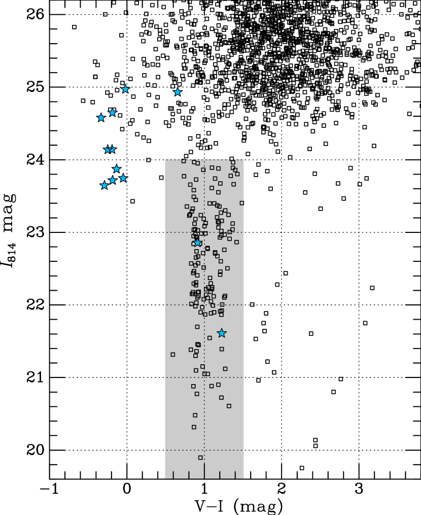
Figure 7.— Color-magnitude diagram for compact sources (FWHM $<$ 0$\farcs$2) in the galactocentric radial range $10\arcsec<R_{g}<108\arcsec$. The shaded region marks the broadest selection we use for GC candidates: $0.5<(V{-}I)<1.5$ and $I_{814}<24$. The blue stars represent compact sources with $I_{814}<25$ that lie within the H ii regions identified by Meurer et al. (2006). The two such sources that lie within the region of the GC candidates are probably simple cases of projection. In general, objects with $(V{-}I)\approx 0\pm 0.5$, $I_{814}\approx 23.5$–25.5 appear to be blue supergiants either in the H ii regions or dispersed along the faint spiral arms; those with $(V{-}I)\approx 2$, $I_{814}<23$ are likely Galactic M dwarfs. The large cloud of points with $(V{-}I)\approx 2\pm 0.1$ and $I_{814}\gtrsim 25$ are (mostly blends of) the brightest evolved giants and supergiants in NGC 1533.

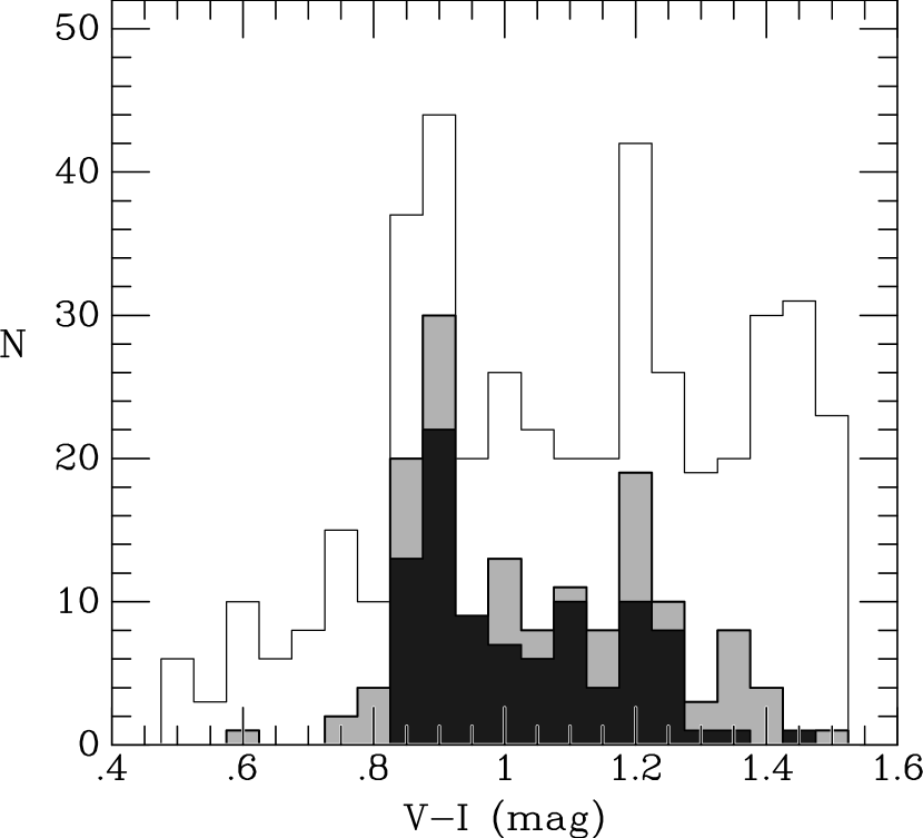
Figure 8.— Histograms of candidate globular cluster $(V{-}I)$ colors (converted from F814W and F606W as described in the text). The gray histogram uses an $I$-band magnitude cutoff $I<24$ (about 1$\,\sigma$ beyond the peak of the GCLF) with the FWHM and radial position selections as given in Figure 7. The open histogram is similar, but uses a cutoff $I<26$, and thus has a substantial contribution from the brightest giants in NGC 1533. The dark histogram includes only the $I<23$ GC candidates that are found to be nonstellar based on the ISHAPE fits, and thus should be nearly free from contamination.

The selection for GC candidates was done for the catalogs from each pointing, then the two lists of GC candidates were merged, giving a total of 151 candidates. For objects in the overlapping region of the two roll angles, the objects’ magnitudes and colors were averaged. Table 2 lists the positions, $(V{-}I)$ colors, effective radii (discussed in the following section), $I_{814}$ magnitudes, and field (roll 1, roll 2, or merge) for each object selected in this way. Figure 8 shows a histogram of the color distribution of these objects. For comparison, it also shows the distribution when the magnitude cutoff is $I_{814}=26$, and the distribution for a cutoff of $I_{814}=23$ with apparently stellar sources (based on the shape fits in Sec. 6.1) removed. For the former sample ($I_{814}{<\,}26$), there is sizable contamination from the faint red sources seen in Figure 7, while for the latter sample ($I_{814}{<\,}23$, nonstellar), there should be negligible contamination.

The $(V{-}I)$ distribution of the GC candidates (gray histogram in Figure 8) was tested for bimodality using the KMM (Kaye’s Mixture Modeling) algorithm (McLachlan & Basford 1988; Ashman et al. 1994), which compares the goodness-of-fit between single and double Gaussian descriptions of the data. The algorithm finds that the data are better described by a double Gaussian with $>99.9$% confidence. It returns best-fit values for the color peaks of 0.921 and 1.226 mag. Assuming the relation for GCs from Kissler-Patig et al. (1998), these correspond to peak metallicities $[{\rm Fe/H}]\sim-1.5$ and $\sim-0.5$, which are normal for a galaxy of this luminosity (e.g., Fig. 13 of Peng et al. 2006). We also considered restricting the GC candidates to a narrower color range of $0.7\leq(V{-}I)\leq 1.4$ (since the Gaussian assumption makes the method sensitive to outliers) and to alternative magnitude cutoffs of $I_{814}<23$ and $I_{814}<25$, as well as excluding the small percentages of likely stellar objects among the candidates. The confidence of bimodality (in the KMM sense) remained near 100% for all these combinations of magnitude and color cuts, except for the case with the faint magnitude cut $I_{814}<25$ and broader color range of $0.5\leq(V{-}I)\leq 1.5$, for which the confidence level was 98.8%. This fainter cutoff results in considerable contamination, yet still exhibits likely bimodality. We conclude that the GC color distribution in NGC 1533 is bimodal to a high level of confidence.

Figure 9.— $(V{-}I)$ colors for GC candidates in the red (filled squares) and blue (open squares) peaks, as determined by the KMM algorithm, are plotted as a function of $I_{814}$ magnitude. The solid lines show the average colors for the two groups. There is no significant slope in the color-magnitude relations of either the red or blue GCs when a cutoff magnitude of $I_{814}<23$ is used.

Recently there has been discussion in the literature of a correlation between magnitude and color for the blue component of the GC population in some galaxies, in the sense that the blue GCs become redder at higher luminosities (Harris et al. 2006; Strader et al. 2006; Mieske et al. 2006). This has been dubbed “the blue tilt.” As a simple test for this in NGC 1533, we split our catalog of GC candidates into red and blue groups using the $(V{-}I)=1.07$ average between the two peaks from KMM as the dividing value. We then performed simple linear least-squares fits to test for a nonzero slope (see Figure 9). With a magnitude cutoff of $I_{814}<23$, (just beyond the peak of the GCLF), we find slopes of $d(V{-}I)/dI=0.003\pm 0.012$ and $d(V{-}I)/dI=0.012\pm 0.021$ for the color-magnitude relations of the blue and red GC candidates, respectively; both are zero within the errors. If we use a cutoff magnitude of $I_{814}<24$, then the slopes both differ from zero by 2$\,\sigma$, but this occurs as a result of the increasing scatter at fainter magnitudes, coupled with the truncation of the other half the data (simple tests can reproduce this effect). When observed, the “tilt” occurs because the blue and red sequences converge at bright magnitudes, not diverge at faint magnitudes. There is no evidence of this effect in the present data set.

The lack of the blue tilt for NGC 1533 is not surprising, since past evidence for it comes from GCs in the brightest ellipticals in galaxy groups and clusters (Harris et al. 2006; Mieske et al. 2006). In such systems, the GCs reach higher luminosities and masses, both because the populations are richer and because the GCLFs are broader (Jordán et al. 2006). The simplest explanation for the tilt is that it results from self-enrichment: the most massive metal-poor GCs were able to retain some self-enriched gas while star formation was ongoing. Since the GCs in a small population like that of NGC 1533 do not reach such high masses, this effect may not have occurred. For instance, Harris et al. (2006) report that for very bright galaxies, the blue and red GC peaks merge into a single broad peak at $M_{I}<-10.5$. In NGC 1533, only 7 GC candidates have this high luminosity ($I\lesssim 20.9$), so it impossible to discern if the blue and red peaks merge. Similarly, if the tilt is due to mergers or accretion by GCs, it might only occur in the richest systems where these would be more common. It will be interesting to see if blue tilts are found in the GC systems of other intermediate-luminosity galaxies, and if so, whether those systems are unusually rich or have broad GCLFs.

6. Globular Cluster Sizes

6.1. GC Shape Analysis

The half-light radius of each GC candidate was obtained using the Ishape program (Larsen 1999). Ishape fits the 2-D shape of each object under the assumption that the object can be modeled by one of various analytic profiles convolved with the PSF. We fitted the GC candidates in each roll using the “KING30” profile, which is a King (1962) model with concentration parameter $c=30$. Ishape reports the model FWHM in pixels (prior to PSF convolution), which we then converted to effective radius $R_{\rm eff}$ using the conversion factor of 1.48 given in Table 3 of the Ishape users’ manual (Larsen 2005). We then converted to a physical size in parsecs using the distance derived in Sec. 4. From this analysis, 12 of the 151 GC candidates (7.9%) brighter than $I_{814}{=\,}24$ were found to be stellar, with zero intrinsic size, and were then removed from the catalog.

We fitted the GC candidates (and fainter sources to $I_{814}<26$) for the two different roll angles separately, then compared the results for sources in the overlapping region. This is an important test, as Ishape does not provide very robust size uncertainties. The manual states that the sizes should be accurate to about 10%, given sufficiently high signal-to-noise ($S/N\gtrsim 40$). Figure 10 shows that the agreement is good down to $I_{814}=23$, where the scatter in the differences is 0.4 pc (or 0.3 pc error per measurement), but worsens abruptly at fainter magnitudes. The scatter is larger by a factor of 7.5 for objects with $23<I_{814}<24$, and by a factor of 10 for $23<I_{814}<26$. We therefore consider only objects with $I_{814}<23$ as having reliable $R_{\rm eff}$ determinations, although we tabulate all the measurements in Table 2.

Figure 11 compares the effective radii from roll 1 to those from roll 2 for objects with $I_{814}<23$ and present in both observations. The RMS scatter in the differences is 18.9%, indicating that the error per measurement is 13%. There is no significant offset in the $R_{\rm eff}$ values measured in the two different observations.

Figure 10.— Differences in the $R_{\rm eff}$ values from Ishape for matched objects present in both the roll 1 and roll 2 observations are plotted as a function of $I_{814}$ magnitude. There is an apparent abrupt transition from reliable to dubious measurement values at $I_{814}\approx 23$.

Figure 11.— Top: Measured $R_{\rm eff}$ values for objects with $I_{814}<23$ in roll 1 are plotted against the $R_{\rm eff}$ values for the same objects measured in roll 2. The plotted line is equality. Bottom: Fractional differences in the $R_{\rm eff}$ values are plotted as a function of the average value. The solid line shows the mean offset of $0.038\pm 0.036$.

Figure 12.— Left: GC effective radius is plotted versus GC color, showing no significant correlation. Right: GC effective radius is plotted versus radius from the center of NGC 1533. The line shows the correlation given in Eq. 5, which has a slope of $\sim\,$0.2 pc/kpc.

Some previous studies have found that $R_{\rm eff}$ depends on the color of the GC, with red GCs being smaller on average than blue GCs (Jordán et al. 2005; Larsen et al 2001). Figure 12 (left panel) shows $R_{\rm eff}$ vs $(V{-}I)$ for all GCs brighter than $I_{814}=23$ in both roll angles (with the values averaged for objects in the overlap). We find no statistically significant trend of $R_{\rm eff}$ with color in the present data set. However, the sample consists of only 92 objects with robust $R_{\rm eff}$ measurements. If we calculate the median $R_{\rm eff}$ values for the 56 blue GCs and 36 red GCs (using the KMM splitting from above), we find $\langle R_{\rm eff}\rangle=2.90\pm 0.13$ and $\langle R_{\rm eff}\rangle=2.59\pm 0.18$ for the blue and red GCs, respectively. The uncertainties have been estimated by dividing the robust biweight scatter (Beers et al. 1990) by the square root of the number in each sample. Thus, we find that the red GCs are $11\pm 8\%$ smaller than the blue ones, which is in the expected sense but not very significant.

On the other hand, we do find a correlation between $R_{\rm eff}$ and radial distance from center of NGC 1533 (Figure 12, right panel). The average size of the GCs increases with galactocentric radius. Omitting the 3 objects at radius $\sim 0\farcm 5$ with $R_{\rm eff}>9$ pc (which are more than 6$\,\sigma$ outliers), we find the following relation:

$$R_{\rm eff}\;=\;(2.83\pm 0.12)\,+\,(0.191\pm 0.047)[(R_{g}/1\,{\rm kpc})-4]\;{\rm pc},$$ (5)

where $R_{\rm eff}$ is in pc and galactocentric radius $R_{g}$ is in kpc. The best-fit slope is virtually unchanged if the blue and red GCs are taken separately: $0.18\pm 0.06$ and $0.20\pm 0.08$ for blue and red, respectively. Thus, we find a strong correlation between $R_{\rm eff}$ and radius $R_{g}$, significant at the 4$\,\sigma$ level, but no significant correlation between $R_{\rm eff}$ and color. NGC 1533 is much more similar to the Milky Way in this regard (e.g., van den Bergh et al. 1991) than to the early-type galaxies in the Virgo cluster, where $R_{\rm eff}$ has only a mild dependence on $R_{g}$ but a significant dependence on color (Jordan et al. 2005). It is tempting to associate this difference with environment, but first it is necessary to study the behavior of $R_{\rm eff}$ for the GCs of many more galaxies in loose group environments.

6.2. Distance from Half-Light Radius

Using the extensive ACS Virgo Cluster Survey data set, Jordan et al. (2005) have proposed a distance calibration based on the median half-light radius of the GC population of a galaxy. From Eq. 19 of that paper, the distance $d$ in Mpc to the galaxy is estimated as

$$d=\frac{0.552\pm 0.058}{\langle\hat{r}_{h}\rangle}\;\hbox{Mpc},$$ (6)

where $\langle\hat{r}_{h}\rangle$ is the corrected median half-light radius in arcseconds (their $r_{h}$ corresponds to what we have called $R_{\rm eff}$, following the Ishape notation). Their definition of $\langle\hat{r}_{h}\rangle$ involves small corrections based on galaxy $z$-band surface brightness, galaxy $(g{-}z)$ color, and GC $(g{-}z)$ color. We do not have photometry in these bandpasses, and although we might estimate conversions from models, Jordán et al. note that the corrections are second-order; one can omit them for bright galaxies such as NGC 1533 and still obtain an accurate distance. Thus, we simply take $\langle\hat{r}_{h}\rangle$ as equal to the median $\langle R_{\rm eff}\rangle=0\farcs 0296\pm 0\farcs 0011$ for the 92 GC candidates in our catalog with $I_{814}<23$. This gives a distance $d=18.6\pm 2.0$ Mpc, in accord with the distance of $19.4\pm 1.1$ Mpc obtained from SBF in Sec. 4. The agreement in distance implies that the sizes of the GCs in NGC 1533 agree in the median with those in the Virgo cluster and supports the use of GC half-light radii as distance indicators.

Figure 13.— The GCLF of candidate globular clusters. The thick solid curve is a maximum likelihood fit to the (unbinned) GC magnitude distribution, represented by the histogram. The dashed line shows the limiting magnitude used for the fit.

Figure 14.— Probability contours on the GCLF width $\sigma$ and turnover magnitude $m^{0}_{I}$ from the maximum likelihood fitting routine. The contours are drawn at significance steps of 0.5 $\sigma$, with the outermost being at 3$\,\sigma$ (99.7% confidence).

7. Globular Cluster Luminosity Function

We used the maximum likelihood code from Secker (1992) to fit the globular cluster luminosity function (GCLF) for 151 GC candidates down to a limit of $I_{814}=24$. In order to do this, it is necessary to have a reasonable estimate of the background contamination. We searched the HST archive for possible background fields with similar Galactic latitudes ($b\approx-45$) taken through the same F606W+F814W filter combination to a similar depth. These fields were processed in the same way as the NGC 1533 fields, and the catalogs were subjected to the same selection according to their magnitude, color, and FWHM. Some of these fields were found to be anomalously rich, as they targeted distant rich galaxy clusters; these fields were excluded. In the end, we used three high-latitude background comparison fields from HST program numbers 9405, 9919, and 10438.

For a Gaussian GCLF, we find a turnover (peak) $I_{814}$ magnitude $m^{0}_{I}=22.84^{+0.18}_{-0.24}$ and dispersion $\sigma_{\rm LF}=1.10\pm 0.15$ mag. This GCLF is plotted in Figure 13. The code also reports the confidence contours on the fit, as shown in Figure 14. We performed various tests by changing the selection of the data, including narrowing the color range to be between 0.7 and 1.4, varying the cutoff magnitude by $\pm 0.5$ mag, and being more restrictive with the FWHM cut. These alternative selections changed $m^{0}_{I}$ by about $\pm 0.1$ mag, and $\sigma_{\rm LF}$ by about $\pm 0.05$ mag, both well within the quoted errors.

Our SBF distance together with the measured $m^{0}_{I}$ implies $M^{0}_{I}=-8.6^{+0.22}_{-0.27}$ for NGC 1533. Conversely, the GCLF measurement provides another estimate of the distance, if we have a calibration for $M^{0}_{I}$. Harris (2001) gives a $V$-band calibration $\langle M^{0}_{V}\rangle=-7.4\pm 0.2$, where we use the quoted scatter as an estimate of the uncertainty. This zero point assumes a Virgo distance modulus of 30.97, which is 0.12 mag less than the calibration used for the ACS Virgo Cluster Survey and in this work. If we adjust for this offset and assume $\langle V{-}I\rangle$ = 1.07 mag (Sec. 5; Gebhardt & Kissler-Patig 1999), then we have $\langle M^{0}_{I}\rangle=-8.59$, giving $(m{-}M)=31.41\pm{0.29}$ mag. This is consistent with the measured SBF distance and the distance estimated from the GC half-light radii. Note, however, that if we had used the value of $\langle M^{0}_{V}\rangle$ given by Harris for S0 galaxies, or if we had converted from the value of $\langle M^{0}_{z}\rangle$ given by Jordán et al. (2006), then the inferred distance modulus would have been larger by about 0.2 mag, although still in agreement within the errors.

Jordán et al. (2006) have found a correlation for Virgo galaxies of the GCLF width with galaxy $B$ luminosity, and we can test whether or not NGC 1533 follows this trend. The total apparent $B$-band magnitude of NGC 1533 from the RC3 is 11.7. With our measured $(m{-}M)$, Eq. (2) from Jordán et al. (2006) predicts $\sigma_{\rm LF}=1.09$ mag, in excellent agreement with our measured value of $1.10\pm 0.15$ mag. We conclude that the GCLF of NGC 1533 is consistent within the uncertainties with those observed in Virgo.

Finally, we can estimate the value of the GC specific frequency $S_{N}=N_{\rm GC}\times 10^{0.4(M_{V}+15)}$ (Harris & van den Bergh 1981), where $N_{\rm GC}$ is the number of globulars and $M_{V}$ is the absolute magnitude of the galaxy. The GCLF analysis indicates that the number of GCs integrated over luminosity is $163\pm 20$ in the region analyzed. We used an outer radial limit of 1$\farcm$8 for this study, but a portion of the area within this radius is missing as a result of the proximity of the galaxy to the image edge at both roll angles (see Fig. 1) and the necessity of omitting the inner 10″. If we assume that the GCs are symmetrically distributed like the galaxy light (although they may have a more extended density profile at large radii), then we estimate a total population $N_{\rm GC}=250\pm 30$ within 1$\farcm$8. The total $V$ magnitude of the galaxy within the same radius is $V=10.75$, and using the measured distance modulus, we find $S_{N}=1.3\pm 0.2$. We expect this is very close to the “global” value, as $\lesssim\,$5% of the light (based on the galaxy profile modeling), and few candidate GCs, are beyond this radius (which motivated the choice of radius). This result for NGC 1533 agrees well with the mean local $S_{N}=1.0\pm 0.6$ reported by Kundu & Whitmore (2001) from HST/WFPC2 imaging of nearby S0 galaxies and the average $S_{N}\approx 1.6$ found by Peng et al. (2007) for intermediate-luminosity early-type (mainly S0) galaxies in Virgo.

8. Summary and Conclusions

We have analyzed deep F606W and F814W images of the galaxy NGC 1533 and its GC population taken at two roll angles with the ACS/WFC on HST. Although it is classified as an early-type barred lenticular galaxy, we found faint spiral structure once a smooth fit to the galaxy isophotes was subtracted. The color map shows faint dust features in the area around the bar and inner disk. Previous ground-based H$\alpha$ imaging had shown that the galaxy disk contains several faint, compact H ii regions. We find that all of these regions have some blue stars associated with them. Four of the H ii regions lie within one of the faint spiral arms, and several other blue stars are spread out within the arm. These observations suggest that NGC 1533 is in the late stages of a transition in morphology from type SBa to SB0.

Transition objects such as NGC 1533 may be the key to understanding the evolution of the morphology-density relation in galaxy clusters, which is often explained as infalling spirals being transformed into S0s by the harsh cluster environment (e.g., Dressler et al. 1997; Postman et al. 2005). However, recent evidence at intermediate redshift indicates that the transitions begin outside the clusters in small group environments through galaxy-galaxy interactions (Moran et al. 2007). Following infall, the intra-cluster medium then serves to expedite the process by removing the remaining cool gas. With NGC 1533, we have a close-up view of this transition in the Dorado group, including interaction with the neighboring galaxies IC 2038/2039 (Ryan-Weber et al. 2004).

From two-dimensional two-component parametric modeling of the galaxy surface brightness, we find a bulge-to-total ratio $B/T\approx 0.42$. The half-light radii of the bulge and disk are $\sim\,$7″ and $\sim\,$46″, respectively. We find a best-fitting Sérsic index $n=2.0$ for the bulge, which can be reasonably approximated by an $r^{1/4}$ law in the 1-D profile. However, the disk has a relatively flat profile over a factor-of-three in radius, from $\sim\,$15″ to $\sim\,$45″, then steepens fairly abruptly beyond $\sim\,$50″. This gives the disk a very low Sérsic index of $n\approx 0.4$, which might result from past high-speed interactions of NGC 1533 within the group environment.

Overall, the color of NGC 1533 is that of an evolved, red population, except in the few, small isolated regions where the blue stars occur. The bulge color is $(V{-}I)\gtrsim 1.22$, similar to cluster ellipticals, and then there is a mild, but significant, linear color gradient throughout the disk. There is a gradual isophotal twist and the isophotes increase in ellipticity out to a semi-major axis distance of 24″, where $\epsilon$ goes above 0.4 before falling sharply again towards the round outer disk. The peak of the $A_{4}$ harmonic term, measuring “diskiness,” occurs at a smaller semi-major axis of 21″. This is because the pointed lens-like isophotes occur inside of the bar.

We measured the SBF amplitude in four broad radial annuli for each of the two observations at different roll angles. A gradient in the SBF amplitude is clearly detected and follows the color gradient (the bluer outer regions have relatively brighter SBF). By matching our ACS photometry against ground-based $(V{-}I)$ data for this galaxy, we have accurately calibrated the SBF measurements to obtain distance moduli. We find excellent agreement among the different annuli but with an offset of 0.04 mag in distance between the two observations. However, the distance error is dominated by systematic uncertainty in the color and calibration zero point. We find a final distance modulus $(m{-}M)=31.44\pm 0.12$ mag, or $d=19.4\pm 1.1$ Mpc.

Candidate globular clusters were selected according to color, magnitude, radial position, and FWHM. Analysis of the color distribution of these objects with the KMM algorithm indicates with a very high degree of confidence that the distribution is bimodal with peaks at $(V{-}I)\approx 0.92$ and 1.22. There is no evidence that the blue GCs become redder at bright magnitudes, the so-called “blue tilt.” The absence of this effect in NGC 1533, an intermediate luminosity galaxy with a small GC population, is consistent with a self-enrichment explanation, since the GCs in such systems do not reach the high masses that they do in richer systems. The sizes of the GC candidates were measured using the Ishape software. By comparing the results from the two different roll angles, we found that the effective (half-light) radii $R_{\rm eff}$ have an accuracy of about 13% down to $I_{814}=23$, but are not reliable beyond this. We did not find a significant trend of $R_{\rm eff}$ with GC color, although the red-peak GCs have a median $R_{\rm eff}$ smaller by $11\pm 8$% than the blue-peak GCs.

However, we did find a significant (4 $\sigma$) trend of $R_{\rm eff}$ with galactocentric radius. In this respect, NGC 1533 is more like the Milky Way than the Virgo early-type galaxies. This may be an effect of the environment: since the sizes of the GCs are limited by the tidal field, and the density gradients will be steeper in small groups such as Dorado or the Local Group, GC sizes should have a stronger dependence on radius in such environments. The dominance of this radial effect may weaken or obscure any relation between size and color. More studies of size and color trends for the GCs of galaxies in loose groups are needed to verify this hypothesis, although this may be difficult because of the low GC populations in such systems. We then used the median half-light GC radius to obtain another estimate of the distance to NGC 1533. Following Jordán et al. (2005), we find $d=18.6\pm 2.0$ Mpc, in good agreement with the SBF distance.

We modeled the $I_{814}$-band GCLF of NGC 1533 as a Gaussian using a maximum likelihood fitting routine. The best-fit peak magnitude $m^{0}_{I}=22.84^{+0.18}_{-0.24}$ corresponds to $M^{0}_{I}\approx-8.6$ for the measured SBF distance, in good agreement with expectations based on other galaxies. The fitted Gaussian dispersion of $\sigma_{\rm LF}=1.10\pm 0.15$ mag is in accord with the relation between $\sigma_{\rm LF}$ and galaxy luminosity found recently by Jordán et al. (2006) for Virgo galaxies. Finally we estimate the GC specific frequency in the analysis region to be $S_{N}=1.3\pm 0.2$, typical for a disk galaxy. We conclude that the GCs in NGC 1533 have the same average size, color, and luminosity within the errors as the Virgo early-type galaxies, but the stronger dependence of size on galactocentric distance is more reminiscent of the Milky Way.

NGC 1533 represents an interesting class of transitional objects, both in terms of morphology and environment. A large, multi-band, systematic study of such systems with HST, similar to the ACS Virgo and Fornax Cluster surveys but focusing on group galaxies, has yet to be undertaken and must await either a revived ACS or Wide Field Camera 3. Such an effort would be extremely valuable in piecing together a more complete picture of the interplay between galaxy structure, globular cluster system properties, and environment.

Table 1SBF Measurements for Various Annuli in NGC 1533

$\langle r\rangle$	$(V{-}I)_{0}$	$\overline{m}_{I,\,1}$	$\overline{m}_{I,\,2}$	$(m{-}M)_{1}$	$(m{-}M)_{2}$
(arcsec)	(mag)	(mag)	(mag)	(mag)	(mag)
3.8	1.2329 $\pm$ 0.0007	30.145 $\pm$ 0.009	30.094 $\pm$ 0.013	31.452 $\pm$ 0.009	31.401 $\pm$ 0.014
9.2	1.2194 $\pm$ 0.0024	30.099 $\pm$ 0.011	30.059 $\pm$ 0.007	31.467 $\pm$ 0.016	31.427 $\pm$ 0.012
17.9	1.2029 $\pm$ 0.0075	30.018 $\pm$ 0.012	29.972 $\pm$ 0.006	31.460 $\pm$ 0.036	31.414 $\pm$ 0.034
32.9	1.1899 $\pm$ 0.0142	29.963 $\pm$ 0.014	29.920 $\pm$ 0.010	31.464 $\pm$ 0.065	31.421 $\pm$ 0.065

Note. — Quoted uncertainties reflect internal measurement error only. See text for discussion of systematic errors and final averaged distance.

Table 2GC Candidates

ID	RA	DEC	$(V{-}I)_{0}$	$\pm$	$R_{eff}$	$I_{814}$	$\pm$	field
Number	(J2000)	(J2000)	(mag)	(mag)	(arcsec)	(mag)	(mag)
13	62.478742	$-$56.109037	1.260	0.042	0.0207	22.759	0.024	merge
20	62.481901	$-$56.108821	1.341	0.079	0.0544	23.777	0.046	merge
30	62.494871	$-$56.107931	0.867	0.028	0.0307	22.467	0.014	merge
141	62.503620	$-$56.108303	1.082	0.025	0.0222	22.180	0.012	r2
175	62.469642	$-$56.111536	0.913	0.052	0.0340	22.856	0.034	merge
199	62.475854	$-$56.111165	0.863	0.049	0.0085	22.950	0.032	merge
219	62.456702	$-$56.113055	0.863	0.088	0.0159	23.580	0.058	merge
391	62.458113	$-$56.114010	0.855	0.037	0.0289	22.176	0.023	merge
424	62.477575	$-$56.112507	1.123	0.034	0.0377	22.120	0.019	merge
428	62.512621	$-$56.109436	1.299	0.025	0.0525	22.503	0.011	r2
443	62.468860	$-$56.113378	1.012	0.036	0.0237	21.869	0.022	merge
467	62.466586	$-$56.113788	1.086	0.046	0.0207	22.049	0.029	merge
472	62.470944	$-$56.113139	1.226	0.033	0.0277	21.610	0.018	merge
556	62.498873	$-$56.111763	0.816	0.036	0.0215	23.248	0.021	r2
566	62.486962	$-$56.112939	1.276	0.084	0.0592	23.898	0.054	r2
616	62.507189	$-$56.111401	0.987	0.045	0.0629	23.863	0.026	r2
785	62.488994	$-$56.114282	0.806	0.080	0.0433	23.231	0.060	merge
883	62.473735	$-$56.116447	0.901	0.050	0.0163	22.738	0.034	merge
1030	62.487940	$-$56.116245	1.093	0.023	0.0296	20.884	0.011	merge
1048	62.491160	$-$56.116023	0.869	0.072	0.0355	23.966	0.052	merge
1151	62.483266	$-$56.117620	0.950	0.024	0.0300	19.897	0.011	merge
1238	62.494429	$-$56.117187	0.895	0.056	0.0696	23.727	0.039	r2
1336	62.474199	$-$56.119748	1.220	0.025	0.0266	20.723	0.013	merge
1388	62.475712	$-$56.120119	0.905	0.026	0.0244	20.775	0.013	merge
1398	62.487527	$-$56.119145	0.907	0.045	0.0455	22.925	0.028	merge
1542	62.472319	$-$56.121682	1.070	0.090	0.0355	23.399	0.065	merge
1550	62.469259	$-$56.122013	1.088	0.054	0.0141	22.218	0.036	r2
1607	62.483549	$-$56.121258	0.901	0.025	0.0289	21.363	0.013	merge
1633	62.490568	$-$56.120816	1.270	0.060	0.0037	23.301	0.033	r2
1645	62.468214	$-$56.122742	1.460	0.085	0.0141	22.868	0.053	r2
1669	62.486759	$-$56.121398	0.858	0.023	0.0281	20.880	0.011	merge
1690	62.483049	$-$56.121813	1.205	0.031	0.0252	21.911	0.017	merge
1692	62.489449	$-$56.121244	1.326	0.045	0.0585	22.910	0.026	r2
1760	62.490182	$-$56.121732	1.141	0.074	0.0185	23.741	0.047	r2
1794	62.459528	$-$56.124760	1.046	0.026	0.0170	21.050	0.013	merge
1822	62.493954	$-$56.121881	0.900	0.038	0.0340	22.935	0.023	r2
1837	62.482462	$-$56.122994	0.839	0.057	0.0348	23.287	0.039	merge
1847	62.497809	$-$56.121721	0.834	0.025	0.0511	22.013	0.013	r2
1977	62.466685	$-$56.125414	1.269	0.041	0.0240	22.123	0.025	merge
1980	62.475828	$-$56.124632	0.892	0.036	0.1017	22.274	0.022	merge
2004	62.467446	$-$56.125627	1.042	0.055	0.0333	22.783	0.036	merge
2023	62.495436	$-$56.123193	1.183	0.054	0.0237	23.552	0.033	r2
2032	62.472654	$-$56.125346	0.928	0.027	0.0400	21.448	0.015	merge
2043	62.483985	$-$56.124394	0.893	0.024	0.0281	21.098	0.012	merge
2101	62.480199	$-$56.125032	0.882	0.050	0.1343	23.042	0.033	merge
2138	62.460701	$-$56.127096	1.367	0.058	0.0474	23.121	0.035	merge
2215	62.486362	$-$56.125426	0.819	0.095	0.0585	23.657	0.045	merge
2262	62.472163	$-$56.127100	0.831	0.041	0.0281	22.571	0.026	merge
2321	62.496776	$-$56.125300	0.857	0.029	0.0244	22.439	0.015	r2
2536	62.470591	$-$56.129244	0.884	0.030	0.0222	21.981	0.017	merge
2613	62.474279	$-$56.129425	0.994	0.033	0.0211	22.078	0.018	merge
2657	62.484181	$-$56.128924	1.222	0.028	0.0274	21.865	0.014	r2
2664	62.494131	$-$56.128090	1.215	0.045	0.0562	23.272	0.025	r2
2720	62.475693	$-$56.130236	1.004	0.172	0.0333	21.053	0.012	merge
2753	62.515850	$-$56.126848	1.195	0.035	0.0895	23.355	0.017	r2
2782	62.509445	$-$56.127683	1.129	0.036	0.0385	23.399	0.019	r2
2804	62.467737	$-$56.131626	0.826	0.024	0.0340	21.384	0.012	r2
2846	62.510464	$-$56.128097	0.864	0.024	0.0326	22.293	0.011	r2
2884	62.462936	$-$56.132600	0.918	0.030	0.0266	22.174	0.016	r2
2959	62.466327	$-$56.132967	1.023	0.030	0.0296	22.141	0.016	r2
3108	62.470197	$-$56.133570	0.890	0.051	0.0141	23.448	0.033	r2
3287	62.479226	$-$56.134192	0.841	0.025	0.0451	22.151	0.013	r2
3702	62.464106	$-$56.138694	0.896	0.025	0.0681	22.311	0.012	r2
4233	62.482340	$-$56.141013	0.739	0.045	0.0710	23.773	0.025	r2
4244	62.494051	$-$56.140087	0.861	0.028	0.0296	22.841	0.014	r2
4269	62.504504	$-$56.139280	0.875	0.031	0.0237	23.117	0.015	r2
4737	62.473405	$-$56.145470	0.912	0.020	0.0437	21.459	0.009	r2
4740	62.493197	$-$56.143711	1.069	0.023	0.0296	21.544	0.009	r2
4791	62.482879	$-$56.145036	0.961	0.032	0.0385	22.984	0.015	r2
2072	62.413458	$-$56.114438	0.775	0.032	0.0244	23.354	0.017	r1
2617	62.429086	$-$56.100548	1.128	0.021	0.0451	21.899	0.009	r1
2645	62.422291	$-$56.111412	1.225	0.020	0.0340	21.391	0.009	r1
2859	62.433442	$-$56.097663	1.207	0.045	0.0511	23.672	0.021	r1
3048	62.430437	$-$56.105507	1.103	0.023	0.0385	22.242	0.011	r1
3055	62.425954	$-$56.112310	0.956	0.034	0.0385	23.236	0.018	r1
3110	62.427170	$-$56.111496	0.864	0.039	0.0437	23.489	0.022	r1
3125	62.427697	$-$56.110888	1.018	0.032	0.0222	23.128	0.018	r1
3143	62.428683	$-$56.109900	0.866	0.017	0.0585	20.316	0.007	r1
3540	62.430444	$-$56.113735	0.925	0.023	0.0340	22.125	0.012	r1
3645	62.443910	$-$56.095340	0.914	0.047	0.0511	23.949	0.025	r1
3647	62.430762	$-$56.115511	1.139	0.030	0.0296	22.708	0.015	r1
3978	62.440401	$-$56.106818	1.015	0.036	0.0170	22.986	0.021	r1
4063	62.433704	$-$56.118506	0.920	0.028	0.0340	22.574	0.016	r1
4114	62.436845	$-$56.114726	1.074	0.029	0.0340	22.371	0.015	r1
4202	62.454829	$-$56.089105	0.927	0.022	0.0363	22.181	0.010	r1
4277	62.442072	$-$56.110460	1.099	0.074	0.0340	23.892	0.047	r1
4280	62.440208	$-$56.113842	1.271	0.022	0.0266	21.119	0.011	r1
4320	62.436274	$-$56.121193	1.004	0.039	0.0266	23.086	0.023	r1
4373	62.449126	$-$56.102981	0.885	0.037	0.0725	23.182	0.022	r1
4436	62.453844	$-$56.097291	0.919	0.026	0.0681	22.667	0.013	r1
4444	62.447418	$-$56.107243	1.044	0.029	0.0274	22.096	0.015	r1
4526	62.444006	$-$56.113942	1.260	0.030	0.0525	22.102	0.016	r1
4630	62.444749	$-$56.114977	1.205	0.035	0.0237	22.418	0.020	r1
4658	62.449950	$-$56.107424	1.203	0.043	0.0244	22.930	0.025	r1
4704	62.451416	$-$56.106083	1.098	0.061	0.0163	23.611	0.040	r1
4742	62.460552	$-$56.093062	1.112	0.021	0.0340	21.993	0.009	r1
4760	62.450792	$-$56.108034	1.379	0.078	0.0858	23.664	0.045	r1
4790	62.454256	$-$56.103414	0.909	0.026	0.0311	21.698	0.013	r1
4794	62.453328	$-$56.104755	1.171	0.036	0.0266	22.670	0.020	r1
4806	62.452688	$-$56.106034	1.164	0.049	0.0340	23.206	0.030	r1
4813	62.453102	$-$56.105470	1.167	0.053	0.0770	23.371	0.032	r1
4888	62.460404	$-$56.095814	1.182	0.062	0.0585	23.881	0.036	r1
4948	62.442253	$-$56.124977	1.024	0.029	0.0503	22.215	0.016	r1
5095	62.449093	$-$56.117356	0.884	0.048	0.0451	22.977	0.032	r1
5239	62.450679	$-$56.117956	1.045	0.046	0.0400	22.773	0.029	r1
5271	62.448478	$-$56.121895	1.364	0.056	0.1347	23.041	0.032	r1
5280	62.450171	$-$56.119649	1.188	0.056	0.0466	23.132	0.036	r1
5290	62.457697	$-$56.108462	0.974	0.029	0.0385	21.967	0.016	r1
5313	62.449563	$-$56.121180	1.400	0.096	0.0266	23.858	0.061	r1
5389	62.449014	$-$56.123932	0.882	0.021	0.0326	20.481	0.010	r1
5393	62.455059	$-$56.114635	1.214	0.045	0.0133	22.601	0.028	r1
5446	62.463440	$-$56.103252	1.140	0.035	0.0170	22.725	0.020	r1
5475	62.460226	$-$56.108876	1.226	0.029	0.0969	21.923	0.016	r1
5604	62.450771	$-$56.125846	1.230	0.029	0.0422	22.006	0.016	r1
5708	62.463336	$-$56.108916	0.905	0.047	0.0215	22.901	0.031	r1
5754	62.463867	$-$56.109087	1.221	0.052	0.1199	22.956	0.032	r1
5768	62.452947	$-$56.125993	0.952	0.034	0.0385	21.897	0.016	r1
5837	62.456743	$-$56.121757	0.887	0.026	0.0281	21.300	0.014	r1
5865	62.469218	$-$56.103303	1.208	0.030	0.0681	22.459	0.016	r1
5963	62.455278	$-$56.127144	0.887	0.038	0.0141	22.545	0.024	r1
6042	62.466243	$-$56.111291	1.341	0.120	0.0067	23.842	0.077	r1
6050	62.469475	$-$56.107693	1.184	0.022	0.0296	20.902	0.011	r1
6052	62.472359	$-$56.103277	1.100	0.028	0.0237	22.218	0.015	r1
6055	62.474468	$-$56.100142	0.918	0.033	0.0237	23.026	0.019	r1
6058	62.458180	$-$56.124987	1.226	0.061	0.0340	23.158	0.038	r1
6179	62.474633	$-$56.101859	1.084	0.027	0.0237	22.296	0.014	r1
6279	62.473238	$-$56.107092	1.177	0.051	0.0200	23.148	0.032	r1
6429	62.474914	$-$56.107999	1.263	0.047	0.0385	22.968	0.029	r1
6457	62.475410	$-$56.108026	0.856	0.031	0.0296	22.152	0.018	r1
6597	62.484653	$-$56.097083	1.222	0.031	0.0525	23.020	0.015	r1
6622	62.480808	$-$56.099170	1.087	0.023	0.0266	21.884	0.010	r1
6842	62.480776	$-$56.108464	0.986	0.038	0.0170	22.715	0.023	r1
6872	62.490483	$-$56.094283	0.853	0.033	0.0599	23.327	0.016	r1
6997	62.483392	$-$56.107559	1.183	0.042	0.0244	23.067	0.025	r1
7017	62.471658	$-$56.125870	0.971	0.044	0.0215	22.527	0.028	r1
7081	62.484164	$-$56.108342	0.910	0.030	0.0340	22.408	0.017	r1
7213	62.476729	$-$56.122510	0.841	0.054	0.0503	23.030	0.036	r1
7455	62.494309	$-$56.100625	0.945	0.036	0.0296	22.844	0.018	r1
7509	62.494724	$-$56.101300	0.892	0.026	0.0363	22.653	0.013	r1

References

- Ajhar et al. (1997) Ajhar, E. A., Lauer, T. R., Tonry, J. L., Blakeslee, J. P., Dressler, A., Holtzman, J. A., & Postman, M. 1997, AJ, 114, 626
- Ashman et al. (1994) Ashman, K. M., Bird, C. M., & Zepf, S. E. 1994, AJ, 108, 2348
- Ashman & Zepf (1998) Ashman, K. M., & Zepf, S. E. 1998, Globular Cluster Systems (New York: Cambridge University Press)
- Beasley et al. (2002) Beasley, M. A., Baugh, C. M., Forbes, D. A., Sharples, R. M., & Frenk, C. S. 2002, MNRAS, 333, 383
- Beers, Flynn, & Gebhardt (1990) Beers, T. C., Flynn, K., & Gebhardt, K. 1990, AJ, 100, 32
- Benítez et al. (2004) Benítez, N., et al. 2004, ApJS, 150, 1
- Bernardi et al. (2002) Bernardi, M., Alonso, M.V., da Costa L.N., Willmer, C.N.A., Wegner, G., Pellegrini, P.S., Rité, and Maia, M.A.G. 2002, AJ, 123, 2990
- Bertin & Arnouts (1996) Bertin, E., & Arnouts, S. 1996, A&AS, 117, 393
- Blakeslee et al. (1999) Blakeslee, J. P., Ajhar, E. A., & Tonry, J. L. 1999, Post-Hipparcos Cosmic Candles, 237, 181
- Blakeslee et al. (2003) Blakeslee, J. P., Anderson, K. R., Meurer, G. R., Benítez, N., & Magee, D. 2003, Astronomical Data Analysis Software and Systems XII, 295, 257
- Blakeslee et al. (2002) Blakeslee, J. P., Lucey, J. R., Tonry, J. L., Hudson, M. J., Narayanan, V. K., & Barris, B. J. 2002, MNRAS, 330, 443
- Blakeslee et al. (2001) Blakeslee, J. P., Vazdekis, A., & Ajhar, E. A. 2001, MNRAS, 320, 193
- Brown et al. (2005) Brown, T. M., et al. 2005, AJ, 130, 1693
- Buta et al. (2006) Buta, R., Corwin, H., & Odewahn, S. 2006, The De Vaucouleurs Atlas of Galaxies (Cambridge: Cambridge Univ. Press)
- Cantiello et al. (2005) Cantiello, M., Blakeslee, J. P., Raimondo, G., Mei, S., Brocato, E., & Capaccioli, M. 2005, ApJ, 634, 239
- Cantiello et al. (2007) Cantiello, M., Raimondo, G., Blakeslee, J.P., Brocato, E., & Capaccioli, M. 2007, ApJ, 662, 940
- Côté et al. (2004) Côté, P., Blakeslee, J.P., Ferrarese, L., Jordán, A., Mei, S., Merritt, D., Milosavljević, M., Peng, E.W., Tonry., J.L., & West, M.J. 2004, ApJS, 153, 223
- de Vaucouleurs et al. (1991) de Vaucouleurs, G., de Vaucouleurs, A., Corwin, H. G., Jr., Buta, R. J., Paturel, G., & Fouqué, P. 1991, Third Reference Catalog of Bright Galaxies (New York: Springer-Verlag) (RC3)
- Dressler et al. (1997) Dressler, A., et al. 1997, ApJ, 490, 577
- Drinkwater et al. (2000) Drinkwater, M. J., Jones, J. B., Gregg, M. D., & Phillipps, S. 2000, Publications of the Astronomical Society of Australia, 17, 227
- Ferguson & Sandage (1990) Ferguson, H.C., & Sandage, A. 1990, AJ, 100, 1
- Ferrarese et al. (2006) Ferrarese, L., et al. 2006, ApJS, 164, 334
- Firth et al. (2006) Firth, P., Evstigneeva, E.A., Jones, J.B., Drinkwater, M.J., Phillips, S., & Gregg, M.D. 2006, MNRAS, 372, 1856
- Freedman et al. (2001) Freedman, W. L., et al. 2001, ApJ, 553, 47
- Gebhardt & Kissler-Patig (1999) Gebhardt, K. & Kissler-Patig, 1999, AJ, 118, 1526
- Harris (2001) Harris, W. E. 2001, Saas-Fee Advanced Course 28: Star Clusters, 223
- Harris & van den Bergh (1981) Harris, W. E., & van den Bergh, S. 1981, AJ, 86, 1627
- Harris et al. (2006) Harris, W. E., Whitmore, B. C., Karakla, D., Okoń, W., Baum, W. A., Hanes, D. A., & Kavelaars, J. J. 2006, ApJ, 636, 90
- Haşegan et al. (2005) Haşegan, M., et al. 2005, ApJ, 627, 203
- Jedrzejewski (1987) Jedrzejewski, R. I. 1987, MNRAS, 226, 747
- Jensen et al. (1998) Jensen, J. B., Tonry, J. L., & Luppino, G. A. 1998, ApJ, 505, 111
- Jones et al. (2005) Jones, D.H., Saunders, W., Read, M., & Colless, M. 2005, PASA, 22, 277
- Jordán et al. (2004) Jordán, A., et al. 2004, ApJS, 154, 509
- Jordán et al. (2005) Jordán, A., et al. 2005, ApJ, 634, 1002
- Jordán et al. (2006) Jordán, A., et al. 2006, ApJ, 651, L25
- Jordán et al. (2007) Jordán, A., Blakeslee, J.P., Côté, P., Ferrarese, L., Infante, L., Mei, S., Merritt, D., Peng, E.W., Tonry., J.L., & West, M.J. 2007, ApJS, 169, 213
- Jorgensen (1997) Jorgensen, I. 1997, MNRAS, 288, 161
- Kilborn et al. (2005) Kilborn, V. A., Koribalski, B. S., Forbes, D. A., Barnes, D. G., & Musgrave, R. C. 2005, MNRAS, 356, 77
- King (1962) King, I. 1962, AJ, 67, 471
- Kissler-Patig et al. (1998) Kissler-Patig, M., Brodie, J. P., Schroder, L. L., Forbes, D. A., Grillmair, C. J., & Huchra, J. P. 1998, AJ, 115, 105
- Kravtsov & Gnedin (2005) Kravtsov, A. V., & Gnedin, O. Y. 2005, ApJ, 623, 650
- krist (2003) Krist, J. 2003, ISR ACS-2003-06 (Baltimore: STScI)
- Kundu & Whitmore (2001) Kundu, A., & Whitmore, B. C. 2001, AJ, 122, 1251
- Larsen (1999) Larsen, S. S. 1999, A&AS, 139, 393
- Larsen & Richtler (2000) Larsen, S.S., & Richtler, T. 2000, A&A, 354, 836
- Larsen et al. (2001) Larsen, S. S., Forbes, D. A., & Brodie, J. P. 2001, MNRAS, 327, 1116
- Laurikainen et al. (2006) Laurikainen, E., Salo, H., Buta, R., Knapen, J., Speltincx, T., & Block, D. 2006, AJ, 132, 2634
- Liu et al. (2000) Liu, M. C., Charlot, S., & Graham, J. R. 2000, ApJ, 543, 644
- Mei et al. (2005) Mei, S., et al. 2005, ApJS, 156, 113
- McLachlan & Basford (1988) McLachlan, G. J., & Basford, K. E. 1988, Mixture models. Inference and applications to clustering (Statistics: Textbooks and Monographs, New York: Dekker, 1988)
- Maoz, et al. (1996) Maoz, D., Barth, A.J., Sternberg, A., Filippenko, A.V., Ho, L.C., Macchetto, F.D., Rix, H.-W., & Schneider, D.P. 1996, AJ, 111, 2248
- Meurer et al. (1995) Meurer, G.R., Heckman, T.M., Leitherer, C., Kinney, A., Robert, C., & Garnett, D.R. 1995 AJ, 110, 2665
- Meurer et al. (2006) Meurer, G. R., et al. 2006, ApJS, 165, 307
- Mieske et al. (2006) Mieske, S., et al. 2006, ApJ, 653, 193
- Moran et al. (2007) Moran, S.M., Ellis, R.S., Treu, T., Smith, G.P., Rich, R.M., & Smail I. 2007, ApJ, in press
- Peng, Ho, Impey, & Rix (2002) Peng, C. Y., Ho, L. C., Impey, C. D., & Rix, H. 2002, AJ, 124, 266
- Peng et al. (2006) Peng, E. W., et al. 2006, ApJ, 639, 95
- Peng et al. (2007) Peng, E. W., et al. 2007, ApJ, submitted
- Postman et al. (2005) Postman, M., et al. 2005, ApJ, 623, 721
- Rizzi et al. (2007) Rizzi, L., Tully, R. B., Makarov, D., Makarova, L., Dolphin, A. E., Sakai, S., & Shaya, E. J. 2007, ApJ, 661, 815
- Ryan-Weber et al. (2003) Ryan-Weber, E. V., Webster, R. L., & Staveley-Smith, L. 2003, MNRAS, 343, 1195
- Ryan-Weber et al. (2004) Ryan-Weber, E. V., et al. 2004, AJ, 127, 1431
- Sandage & Brucato (1979) Sandage, A., & Brucato, R. 1979, AJ, 84, 472
- Schlegel et al. (1998) Schlegel, D. J., Finkbeiner, D. P., & Davis, M. 1998, ApJ, 500, 525
- Secker (1992) Secker, J. 1992, AJ, 104, 1472
- Sersic (1968) Sérsic, J. L. 1968, Cordoba, Argentina: Observatorio Astronomico, 1968
- Sirianni et al. (2005) Sirianni, M., et al. 2005, PASP, 117, 1049
- Strader et al. (2006) Strader, J., Brodie, J. P., Spitler, L., & Beasley, M. A. 2006, AJ, 132, 2333
- Tonry et al. (1997) Tonry, J. L., Blakeslee, J. P., Ajhar, E. A., & Dressler, A. 1997, ApJ, 475, 399
- Tonry et al. (2001) Tonry, J. L., Dressler, A., Blakeslee, J. P., Ajhar, E. A., Fletcher, A. B., Luppino, G. A., Metzger, M. R., & Moore, C. B. 2001, ApJ, 546, 681
- van den Bergh et al. (1991) van den Bergh, S., Morbey, C., & Pazder, J. 1991, ApJ, 375, 594
- West et al. (2004) West, M. J., Côté, P., Marzke, R. O., & Jordán, A. 2004, Nature, 427, 31
- Whitmore & Schweizer (1995) Whitmore, B.C., & Schweizer, F. 1995, AJ, 109, 960
- Whitmore et al. (1999) Whitmore, B.C., Zhang, Q., Leitherer, C., Fall, S.M., Schweizer, F., & Miller, B.W. 1999, AJ, 118, 1551