Prediction and verification of indirect interactions in densely interconnected regulatory networks

Abstract

We develop a matrix-based approach to predict and verify indirect interactions in gene and protein regulatory networks. It is based on the approximate transitivity of indirect regulations (e.g. $A\rightarrow B$ and $B\rightarrow C$ often implies that $A\rightarrow C$) and optimally takes into account the length of a cascade and signs of intermediate interactions. Our method is at its most powerful when applied to large and densely interconnected networks. It successfully predicts both the yet unknown indirect regulations, as well as the sign (activation or repression) of already known ones. The reliability of sign predictions was calibrated using the gold-standard sets of positive and negative interactions. We fine-tuned the parameters of our algorithm by maximizing the area under the Receiver Operating Characteristic (ROC) curve. We then applied the optimized algorithm to large literature-derived networks of all direct and indirect regulatory interactions in several model organisms (Homo sapiens, Saccharomyces cerevisiae, Arabidopsis thaliana and Drosophila melanogaster).

Introduction

The development of high-throughput experimental techniques lead to the accumulation of unprecedented amounts of data describing regulatory interactions in model organisms. Effective computational algorithms are needed to convert this treasure trove of information into the system-wide understanding of the underlying biological processes.

Regulatory interactions between proteins can be either direct or indirect. We would refer to a link from a regulatory protein to a target protein as direct if it is mediated by a direct molecular mechanism, such as e.g. transcriptional regulation of target protein’s level by a transcription factor or phosphorylation of a substrate protein by a kinase. Conversely, regulations involving any number of intermediate proteins will be referred to as indirect. In fact, indirect regulations are vastly more common than the direct ones and thus are more likely to be detected experimentally. Large sets of regulatory interactions (both direct and indirect) are often represented in terms of a directed network in which edges carry signs representing whether the regulation is an activation (positive sign) or an inhibition (negative sign). By ignoring the strength of interactions and combinatorial effects of several inputs such network provides a very simplified description of the real-life regulatory processes.

In this work, we develop a novel algorithm which allows one to verify already known indirect regulations, infer their signs (if it is not known), and to predict the new ones, which have not yet been experimentally detected. As an input it uses a network consisting of all presently known regulatory interactions (both direct and indirect). Our algorithm also allows one to make an educated guess about which of the interactions in the original network are direct and which are indirect in cases when this information is not readily available (as e.g. in microarray experiments following a perturbation localized on one or several genes). Thus it contributes to a popular topic of reconstructing direct regulatory network from microarray data Friedman:JCB00 ; Peer:BI01 . Our algorithm works best when applied to large and heavily-interconnected networks. That is the reason we chose to apply it to networks in well-studied model organisms obtained using automatic text-mining technologies Novichkova:BI03 .

Large-scale network analysis of indirect regulatory interactions in yeast was recently studied in Wagner:BI01 ; Wagner:GB04 ; Kyoda:BI04 . These works focused on the classification of regulations as either direct or indirect and subsequently pruning of indirect regulations. Pruning of indirect regulations is a useful procedure from the point of network simplification. However, being developed for relatively sparse networks, these algorithms assume all links are equally reliable and neither of these algorithms performs well for heavily interconnected networks considered in this study.

The emergent behavior of the rapidly growing body of knowledge contained in regulatory and other biomolecular networks was recently explored in a series of publications of Rzhetsky and collaborators Rzhetsky:NatBt05 ; Rzhetsky:PLoS106 ; Rzhetsky:PNAS06 . The matrix-based approach advocated below nicely compliments the Bayesian methods Rzhetsky:PLoS106 of validation of large maps of biomolecular pathways or, more generally, any set of published biological statements Rzhetsky:PNAS06 .

The main idea behind our algorithm is as follows: consider a protein $i$ regulating (either directly or indirectly) a protein $k$ which in its turn is known to regulate (again directly or indirectly) a protein $j$, then it is likely to also have an indirect regulatory interaction between $i$ and $j$. This simple observation could be further extended in two ways. Firstly, indirect regulations could propagate along longer protein cascades, thus a series of regulations $i\rightarrow k_{1}\rightarrow k_{2}\rightarrow j$ contributes to increase the likelihood of an indirect regulation $i\rightarrow j$. Secondly, having multiple parallel pathways reinforce the predictability. Therefore, if a protein $i$ regulates proteins $k_{1}$, $k_{2}$ and each of them regulates a protein $j$, it is even more likely to find an indirect regulation from $i$ to $j$.

A simple-minded way to predict or verify an indirect regulation between a protein $i$ and a protein $j$ is to simply count the number of directed paths connecting $i$ and $j$. However, this counting scheme does not take into account two important observations. First of all, paths should be weighted differently according to their lengths. Inferences based on longer cascades is less reliable, and thus such should contribute less to the likelihood. We choose to exponentially discount longer paths by weighting a path involving $n$ intermediate proteins by a factor $\lambda^{n}$, where $\lambda<1$ is a parameter of our algorithm. Secondly, the inferred sign of the indirect regulation from different paths should agree with each other. In general, if a protein $i$ and a protein $j$ are connected by a multi-step path, the sign of the resultant indirect regulation between $i$ and $j$ is given by the product of signs of all intermediate edges. It is natural to assume that the effect of a positive path (whose edges give a positive product) and the effect of a negative path (whose edges give a negative product) contradict and to some extent cancel each other.

In the next section, we will show that this central idea of predicting likely indirect regulations could be easily incorporated using a matrix formalism. Obviously, the likelihood can serve as a quantitative measure of the reliability of any regulation in a dataset. Thus one could also verify already known regulations based on this calculated likelihood. A regulation with a high likelihood is deemed reliable. On the other hand, indirect regulations with a high likelihood missing from the dataset could be reliably predicted. As always, there is a tradeoff between the number of predictions and their quality.

We applied our algorithm to the set of genetic regulations extracted from contents of the entire PubMed database (14,000,000 abstracts) and 47 full text journals. The automatic extraction of interactions was made possible by the Medscan algorithm based on Natural Language Processing (NLP) techniques Novichkova:BI03 ; Daraselia:BI04 . Both direct and indirect regulatory interactions were collected for four model organisms: Homo sapiens, Saccharomyces cerevisiae, Arabidopsis thaliana and Drosophila melanogaster (see Table 1 for details). As reflected in their inter-connectedness index ($\mathrm{IC}=\langle k^{(in)}k^{(out)}\rangle/\langle k^{(in)}\rangle$), all these networks are globally interconnected (IC$>1$). In particular, since the network of human proteins is the largest and the most heavily interconnected (IC$\simeq$60) among all networks used in this manuscript, we will show the results for this network in more details.

Table 1: Regulatory networks in the four model organisms. The IC (inter-connectedness) index, defined as $\langle k^{(in)}k^{(out)}\rangle/\langle k^{(in)}\rangle$, measures how tightly bound together are the nodes in the network. In this formula $k^{(in)}$ and $k^{(out)}$ stand for the in- and out-degrees of nodes respectively. IC$>1$ means that the network is globally interconnected. From the table one can see that all of the networks used in this study are globally interconnected with the human dataset with IC$\simeq 60$ being the most densely connected of them all. The gold-standard positive and negative sets consist of highly reproducible regulations (the ones reported in multiple publications) with a given sign.

	Number of		Number of links		Size of gold-standard set
Organisms	Proteins	IC	positive	negative	positive	negative
Homo sapiens	7853	61.9	36426	16436	3442	1671
Saccharomyces cerevisiae	1218	3.42	1208	813	125	85
Arabidopsis thaliana	490	2.84	426	252	42	25
Drosophila melanogaster	569	1.39	410	203	46	25

Results and Discussion

Matrix formalism

In this work, we represent the dataset of all known direct and indirect regulatory interactions in a given organism as a directed network. In matrix notation, it is fully defined by an adjacency matrix $A$ taking the values

$$A_{ij}=\left\{\begin{array}[]{l}+1\quad\quad\mbox{if }i\mbox{ positively regulates }j,\\ -1\quad\quad\mbox{if }i\mbox{ negatively regulates }j,\\ \;\;\;0\quad\quad\mbox{if }i\mbox{ is not known to regulate }j.\\ \end{array}\right.$$ (1)

To predict new indirect regulations and to quantify the reliability of the existing ones, we use another matrix $X$ given by

$$X = A^{2}+\lambda A^{3}+\lambda^{2}A^{4}+\lambda^{3}A^{5}\cdots$$ (2)

$$= \frac{A^{2}}{I-\lambda A}$$

where $\lambda<1$ is a parameter to be discussed later. $X_{ij}$ includes the contribution of all paths from $i$ to $j$. $(A^{n})_{ij}$ is the net number of paths (number of positive paths minus the number of negative paths) of length $n$ from node $i$ to node $j$, the sign of $X_{ij}$ is based on whether positive paths or negative paths dominate. If positive (negative) paths dominate, $X_{ij}$ is positive (negative), and it is likely that $i$ is indirectly activating (repressing) $j$.

The constant $\lambda$ in Eq. (2) is basically a free parameter which could be optimized later to provide the best performance for the algorithm. Generally speaking, $\lambda$ determines the weights of different paths. If $\lambda$ is chosen to be less than one, the contribution from long paths is exponential suppressed. In this work, we have chosen different $\lambda$’s for different networks in order to optimize the performance of our algorithm. We will first present our results using the optimal value of $\lambda$. The definition of the optimal $\lambda$ and its determination will be addressed later on.

Calibration of reliability

We have argued that the absolute magnitude of matrix elements of $X$ is a measure of reliability of indirect regulations. Following the matrix formalism, we calculate $X$ for four different regulatory networks: Homo sapiens, Saccharomyces cerevisiae, Arabidopsis thaliana and Drosophila melanogaster (see the Materials and Methods section for additional information).

In our algorithm, every non-zero element of $X$ possesses certain predictive power. We collect all possible predictions by picking out all non-zero $X_{ij}$’s. The validity of our algorithm is evident if pairs $i$ and $j$ with large value of $|X_{ij}|$ are likely to correspond to more reliable regulations. To show this is indeed the case, one needs to use “gold-standard set” containing completely trustable regulations, which however is not readily available. For this purpose, we define the gold-standard set to be regulations which are frequently reported in the literature (for details of the cutoff on the number of publications, see Materials and Methods). The values of the median value of $|X|$ for all the non-zero matrix elements and those within the gold-standard set are $3.9\times 10^{-3}$ and $3.5$ respectively.

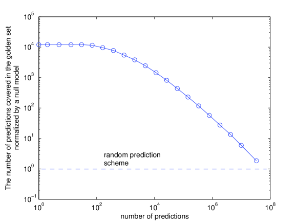
Figure 1: The advantage of our prediction algorithm over null-model expectations. The x-axis corresponds to the number $n$ of predictions with the largest values of $|X_{ij}|$. The y-axis is the ratio between the overlap of these $n$ predictions with the combined (positive+negative) gold-standard set and the null model expectation of this overlap. One can see that our predictions are up to $10^{4}$ times more likely to correspond to reliable, experimentally verified regulations than expected by pure chance alone.

Figure 1 shows a more detailed calibration of the matrix elements. We define a predictive set of size $n$ using the $n$ predictions with the largest values of $|X_{ij}|$. If all the possible predictions are used, the size of the set is huge (up to $10^{7}$). The number of predictions covered in the gold-standard set is counted and normalized by the corresponding number obtained by a set of $n$ random predictions. As shown in Figure 1, the overlap between the gold-standard set and the best $100$ of our predictions is $10,000$ (sic!) times better than what is expected by pure chance alone. The advantage decreases when predictions with smaller values of $|X_{ij}|$ are included. In case all possible predictions are used, the predictive set is only sightly (2-fold) better than a random set. This is expected since predictions with smaller values of $|X_{ij}|$ are much less likely to be reliable.

Large $|X_{ij}|$ is a result of “confirmation” by multi-step paths from $i$ to $j$, therefore such predictions are likely to be indirect in nature. To prove that it is indeed the case, we separate the gold-standard set into direct and indirect subsets based on the information obtained from literature as described. In agreement with our expectation, the predictions are biased toward the indirect subset (see Figure S1 in the Supporting Information).

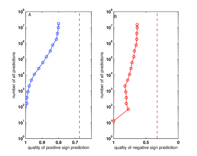
Figure 2: The tradeoff between the number of predictions and their average quality (panel A for positive predictions and B for negative predictions). For a set of predictions, the average quality is defined as the fraction of predictions whose sign agrees with that in the gold-standard set. The dotted line is the quality expected for a null model as described in the main text.

Another use of matrix elements is to determine whether the regulations are positive or negative. Under our formalism, regulations corresponding to large positive matrix elements are likely to represent positive regulations. In order to calibrate the reliability for a set of predictions, we define the average quality by counting the fraction of prediction whose inferred sign agrees with that reported in the gold-standard set. Figure 2 shows the tradeoff between the number of predictions and the average quality. As shown in Figure 2A, a set of predictions with average quality $100\%$ offers about $100$ predictions of positive regulation. However, if one is willing to downgrade the quality to $95\%$, the number of predictions is up to $5000$. By including all the positive entries in $X$, we are offered a huge number of predictions, but with a relatively low quality. However, even in that case, the average quality is still much better than a null model, which is defined as the fraction of positive regulations among all the regulations in the gold-standard set. Thus the quality of our null model for positive (negative) regulations in human is $3442/(3442+1671)=0.67$ ($1671/(3442+1671)$=0.33). They are shown as dashed lines in Figure 2. Using negative matrix elements, one could also predict negative regulations. Large negative elements of $X$ are indeed more likely to have negative signs in our gold-standard set (see Figure 2B).

To understand better the quality of our sign predictions, we study the Receiver Operating Characteristic (ROC) curves. Figure 3A is the ROC curve for positive-sign predictions. It shows the sensitivity against specificity in different predictive sets as described by varying the $|X_{ij}|$ threshold. For positive-sign prediction, sensitivity is defined as the fraction of regulations in the positive gold-standard set which are predicted to be positive by our algorithm. Specificity, on the other hand, is defined as the fraction in the gold-standard negative set that are predicted to be positive by our algorithm. Data points close to the origin consist of predictions with large $X_{ij}$. The most important observation is the convexity of the curve, which means that the sign of interaction predicted by our method is more likely to be correct than expected by pure chance alone. In fact for a totally random predicted set, the ROC curve would be a straight line $y=x$. The area under a ROC curve is commonly used to quantify the performance of an algorithm. Using the negative $X_{ij}$ to predict negative regulations, one could similarly define sensitivity and specificity resulting another ROC curve as shown in Figure 3B.

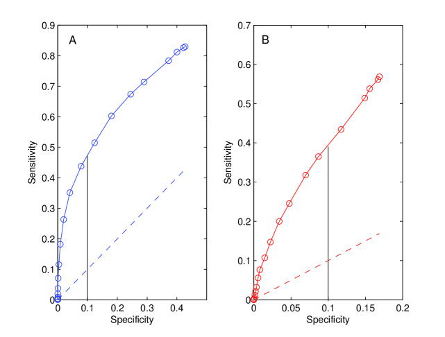
Figure 3: ROC curves for sign predictions using positive $X_{ij}$ (panel A) and negative $X_{ij}$ (panel B). Each data point corresponds to a predictive set defined by a particular threshold of $X_{ij}$. The dotted lines are $y=x$, which is the null model expectations. The area under the ROC curve to the left of the solid line measures the performance of our algorithm.

Making use of the ROC curves, we could address the primary assumption behind our definition of the gold-standard set: the larger is the number of papers reporting a given interaction, the more reliable it is. We define different gold-standard sets by varying the publication cutoff. Gold-standard sets arising from a high cutoff are smaller in size, but supposed to be more reliable. By comparing the area of the ROC curves obtained from different gold-standard sets, we find that indeed the ROC curve from a high-cutoff gold-standard set encloses a larger area (see Figure S2 in Supporting information), which means those regulations are indeed more trustable.

Validation of new predictions

So far, every non-zero matrix element of $X$ stands for a prediction. However, predictions could fall into two categories: those covered in the gold-standard set and those not. Using the predictions covered in the gold-standard set, we have calibrated the reliability. Next, we are going to focus on the predictions missing from the gold-standard set. First of all, we do not consider these regulations as defects. In fact, being in the same predictive set, they possess the same quality as those covered in the gold-standard set. Therefore, we could use them as “real” predictions of missing regulations and expand the original dataset with these predictions.

Table 2 shows the number of the these new predictions offered by our algorithm for the four model organisms. Two different quality cutoffs $95\%$ and $75\%$ are used. The number of predictions offered varies among the datasets, this is because the datasets have different number of nodes, links and topologies. However, in all cases, one could gain more predictions by lowering the quality cutoff. We would like to stress that the term “quality” is calibrated separately in different datasets, therefore it is not meaningful to compare the new predictions in human and yeast even though their apparent qualities are the same. In fact, predictions from human dataset are the most reliable, because our algorithm is benefited from the heavily connected nature of the human dataset.

Without experimental verification, it is hard to validate our new predictions. To demonstrate our new predictions indeed make biological sense, we compare our new predictions from human data to a complementary dataset of human regulatory interactions. The dataset is also obtained from literature using the Medscan algorithm but all the regulations are not included in Table 1 and the matrix $A$ (see the Materials and Methods section). We find that a significant fraction of our new predictions coincide with this dataset. As shown in Table 2, we have generated $2500$ new predictions with an average quality of $95\%$ for the human network. Among them $750$ are indeed verified in the extra dataset. The corresponding P-value with respect to a random model is less than $10^{-100}$. The list of $2500$ predictions in human network, together with the predictions for other model organisms are listed in Table S3 in Supporting information.

Table 2: Number of new predictions offered by our algorithm in regulatory networks of different organisms.

Organisms	95% sign quality	75% sign quality
Homo sapiens	2500	$1.8\times 10^{7}$
Saccharomyces cerevisiae	190	7100
Arabidopsis thaliana	85	13000
Drosophila melanogaster	650	1400

The optimal value of $\lambda$

With ROC curves in hand, we are in a position to choose an appropriate $\lambda$ for Eq. (2). As a common practice, the quality of a ROC curve is quantified by the area under the curve. The optimal $\lambda$ is thus the one whose ROC curve encloses the largest area. However, the direct comparison of different areas may be ambiguous. For example, compare the ROC curves from Fig. 3, the one on the left panel encloses a larger area while at the same time, the length covered in the x-axis is longer. To overcome the problem, we introduce a cutoff in the x-axis, and integrate area from $0$ up to the cutoff. In this study, the cutoff is chosen to be $0.1$. As the beginning of the ROC curve refers to the highly reliable predictions, the introduction of the cutoff restricts ourselves in comparing the most reliable predictions. Thereafter, we define a quantity $\theta$ to measure the overall performance of the algorithm, which is the ratio between the area under the ROC curve from $0$ to the cutoff and the corresponding area under the straight line $y=x$. The ratio could be understood as the advantage of our algorithm over random predictions.

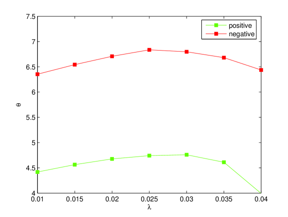
Figure 4: Determination of the optimal value of $\lambda$. Optimal $\lambda$ maximizes $\theta$, defined by the ratio between the area under the ROC curve from $0$ to $0.1$ and the corresponding area under the straight line $y=x$. For human network, the optimal $\lambda$ for positive and negative predictions are $0.025$ and $0.030$ respectively.

The performance of a particular $\lambda$ in Eq. 2 could be quantified by the resultant $\theta$. In Fig. 4, we plot $\theta$ against different $\lambda$’s for positive and negative ROC curves in the human dataset. In short, the optimal $\lambda$ is the one which gives the largest $\theta$. From Figure 4, the optimal $\lambda$ for positive and negative predictions are $0.025$ and $0.030$ respectively. Readers are referred to the Materials and Methods section for details of estimating $\theta$.

Materials and Methods

Collections of regulatory networks

The regulatory networks for different model organisms are obtained by the Medscan algorithm based on Natural Language Processing (NLP). The term “regulation” refers to the general influence of the activity of one protein by another. Therefore, apart from transcriptional regulations (which are direct regulations), indirect regulations might be results of any cascades of post-transcriptional or post-translational interactions between proteins.

Regulations are extracted from over 14 million PUBMED abstracts and 47 full text journals. Properties of regulations including the sign (positive or negative) and its nature (direct and indirect) are parsed whenever the information could be extracted from the corresponding abstract. The number of times a regulation is reported in literature is kept for the definition of gold-standard sets. Details of each network is shown Table 1.

Apart from the data as shown in Table 1, we have extracted an additional set ($35672$) of human regulations. The regulations are not included with the datasets in Table 1 because their signs could not be parsed. In this study, we use them as independent validation for the new predictions generated by our algorithm.

Definition of gold-standard sets

For each organism, the corresponding positive (negative) gold-standard set is defined by the top $10\%$ most frequently reported positive (negative) regulations. The size of each gold-standard set could be found in Table 1. For human dataset, the publication cutoffs used in positive and negative gold-standards are $8$ and $5$ respectively.

Estimation of the area under a ROC curve

For each ROC curve, we fit the data point by the function $y=Ax^{B}$ using the MATLAB function fminsearch, which is based on the Nelder-Mead method in non-linear optimization. The area under the fitted curve is numerically evaluated in MATLAB by the function quadl using the adaptive Lobatto quadrature.

To exclude the data points far from the origin, which are results of less reliable predictions, we introduce a cutoff in the x-axis. Area is integrated from $0$ up to the cutoff. In this study, a cutoff of value $0.1$ is used.

Acknowledgements

Work at Brookhaven National Laboratory was carried out under Contract No. DE-AC02-98CH10886, Division of Material Science, U.S. Department of Energy. This work was supported by National Institute of General Medical Sciences Grant 1 R01 GM068954-01. IM thanks the Institute for Strongly Correlated and Complex Systems at Brookhaven National Laboratory for hospitality and financial support during visits when the majority of this work was done. KKY and SM visit to Kavli Institute for Theoretical Physics where part of this work was accomplished was supported by the National Science Foundation under Grant No. PHY05-51164.

Supporting Information

Figure S1. The coverage of direct and indirect gold-standard sets. The coverage of the direct (indirect) subset for a given set of predictions is defined as the number of verified predictions normalized by the size of the direct (indirect) gold-standard set. Data points closer to the origin refer to predictions with larger average value of $|X_{ij}|$. As reflected by the convexity of the curve, those regulations are more likely to be indirect rather than direct.

Figure S2. ROC curves of the human regulatory network using gold-standard sets with different cutoffs. A gold-standard set is defined by regulations which are highly reported in literature. An interaction belonging to the gold-standard set with cutoff $5\%$ is among the top $5\%$ of the dataset in terms of the number of papers reporting. Data points labeled by $\circ$, $\triangle$ and $\star$ are the results of gold-standard sets whose sizes are $5\%$, $10\%$ and $20\%$ of the original network. These correspond to publication cutoffs $14,8,4$ for positive regulations and $9,5,3$ for negative regulations respecitively. The ROC curves (positive and negative) corresponding to a high-cutoff gold-standard set enclose larger areas.

Table S3. The new predictions and their signs offered by our algorithm with an average quality of 95%. (Table_S3.xls)

References

- (1) Friedman N, Linial M, Nachman I, Pe’er D (2000) Using bayesian networks to analyze expression data. J Comput Biol 7:601–620. doi:10.1089/106652700750050961.
- (2) Pe’er D, Regev A, Elidan G, Friedman N (2001) Inferring subnetworks from perturbed expression profiles. Bioinformatics 17 Suppl 1:S215–24.
- (3) Novichkova S, Egorov S, Daraselia N (2003) Medscan, a natural language processing engine for medline abstracts. Bioinformatics 19:1699–1706.
- (4) Wagner A (2001) How to reconstruct a large genetic network from n gene perturbations in fewer than n(2) easy steps. Bioinformatics 17:1183–1197.
- (5) Tringe SG, Wagner A, Ruby SW (2004) Enriching for direct regulatory targets in perturbed gene-expression profiles. Genome Biol 5:R29. doi:10.1186/gb-2004-5-4-r29.
- (6) Kyoda K, Baba K, Onami S, Kitano H (2004) Dbrf-megn method: an algorithm for deducing minimum equivalent gene networks from large-scale gene expression profiles of gene deletion mutants. Bioinformatics 20:2662–2675. doi:10.1093/bioinformatics/bth306.
- (7) Cokol M, Iossifov I, Weinreb C, Rzhetsky A (2005) Emergent behavior of growing knowledge about molecular interactions. Nat Biotechnol 23:1243–1247. doi:10.1038/nbt1005-1243.
- (8) Rzhetsky A, Zheng T, Weinreb C (2006) Self-correcting maps of molecular pathways. PLoS ONE 1:e61. doi:10.1371/journal.pone.0000061.
- (9) Rzhetsky A, Iossifov I, Loh JM, White KP (2006) Microparadigms: chains of collective reasoning in publications about molecular interactions. Proc Natl Acad Sci U S A 103:4940–4945. doi:10.1073/pnas.0600591103.
- (10) Daraselia N, Yuryev A, Egorov S, Novichkova S, Nikitin A, et al. (2004) Extracting human protein interactions from medline using a full-sentence parser. Bioinformatics 20:604–611. doi:10.1093/bioinformatics/btg452.