Water maser variability over 20 years in a large sample of star-forming regions: the complete database

Abstract

Context. Water vapor emission at 22 GHz from masers associated with star-forming regions is highly variable.

Aims. We present a database of up to 20 years of monitoring of a sample of 43 masers within star-forming regions. The sample covers a large range of luminosities of the associated IRAS source and is representative of the entire population of H₂O masers of this type. The database forms a good starting point for any further study of H₂O maser variability.

Methods. The observations were obtained with the Medicina 32–m radiotelescope, at a rate of 4–5 observations per year.

Results. To provide a database that can be easily accessed through the web, we give for each source: plots of the calibrated spectra, the velocity–time–flux density plot, the light curve of the integrated flux, the lower and upper envelopes of the maser emission, the mean spectrum, and the rate of the maser occurrence as a function of velocity. Figures for just one source are given in the text for representative purposes. Figures for all the sources are given in electronic form in the on-line appendix. A discussion of the main properties of the H₂O variability in our sample will be presented in a forthcoming paper.

1 Introduction

Since the discovery of 22 GHz H₂O maser emission associated with young stellar objects (YSOs) within star-forming regions (SFRs), variability of maser emission is well-known. Changes as large as several orders of magnitude in the maser emission have been observed (e.g., Little et al. lit77 (1977); Liljeström et al. lil89 (1989); Claussen et al. cla96 (1996); Comoretto et al. com90 (1990); Wouterloot et al. wou95 (1995)). At the same time, velocity drifts of individual components of up to a few km s^-1 per year have also been reported (e.g., Brand et al. BCCFPPV2003 (2003)). The variability can be slow or burst-like and covers all ranges of timescales, from hours-days to months-years. In the present study we are mainly concerned with the latter and, for the first time, deal with a large sample of sources (43) and with a time-span of up to 20 years, with 4–5 spectra per year.

Due to the large amount of telescope time required to follow the evolution of H₂O maser emission, inevitably the variability is more easily monitored through single dish observations. In fact, besides our campaign only the Pushchino 22–m single-dish maser patrol covers a comparably long period (e.g., Rudnitskij et al. russi (2007)). Furuya et al. (furuya (2003)) carried out a multiepoch 22 GHz H₂O maser survey towards 173 low-mass YSOs (Class 0 to Class III sources) using the Nobeyama 45 m telescope. This was the first complete water maser survey towards Class 0 sources in the northern sky. However, their observations extend non-uniformly over a period of only three years.

It is well-known that the variability depends strongly on the luminosity of the SFR (usually derived from the associated IRAS source). For instance, there is a minimum luminosity ($\sim$25 L_⊙) below which H₂O maser emission may be present only for about one third of the entire duration of the maser activity (Persi et al. per94 (1994); Claussen et al. cla96 (1996)). The results obtained so far suggest that the lower the SFR luminosity, the higher the observed degree of variability of the H₂O maser emission. Higher luminosity sources may show more steady components. Consequently, a large sample of sources is needed to better understand the dependence of the variability on other parameters of the SFRs, in particular on their luminosities which cover a range of several orders of magnitude, and on their (molecular) environment.

The use of a single dish instrument is of course a limitation because interferometric observations clearly show that H₂O  masers within a SFR often consist of many spatially separated, unresolved components, generally clustered in groups (usually with different velocities), which in most cases cannot be separated in single dish observations (e.g., Forster & Caswell for89 (1989),  for99 (1999); Tofani et al. tof95 (1995)). However, Felli et al. (FMRC2006 (2006)) reported a case in which single dish observations were able to separate the evolution of spatially distinct components. Nevertheless, frequent single dish observations have the advantage of being able to follow potential velocity drifts of individual velocity components, which can be easily identified in the spectra, and thus give a better view of the dynamics (e.g., accelerations) occurring in the circumstellar environment of the YSO.

In two earlier papers (Valdettaro et al. VPBCCFP2002 (2002); Brand et al. BCCFPPV2003 (2003)), we set the basis for a systematic study of the H₂O variability in SFRs with the Medicina 32–m radiotelescope using a sample of 14 sources which covered a wide range of luminosities and had been observed for more than 10 years. Here we report on a larger sample of 43 SFRs (including the former 14 sources) and increase the time coverage up to 20 years. The database is presented in the form of plots of the calibrated spectra and additional plots of derived quantities, in a form that can be easily accessed through the web. In a forthcoming paper, we will analyze the properties of H₂O variability of our sample.

2 The sample

A large sample of sources selected from the Arcetri Atlas (Cesaroni et al. cesa88 (1988); Comoretto et al. com90 (1990); Palagi et al. PCC93 (1993); Brand et al. brand (1994); Valdettaro et al. val01 (2001)) has been monitored regularly since the beginning of the operating period of the Arcetri digital autocorrelator at the Medicina 32–m radiotelescope (1987), at a rate of 4–5 observations per year. Our goal was to study the dependence of the variability of H₂O masers in SFRs on the luminosity of the associated YSO, assumed to remain constant during our patrol. It should be pointed out that the FIR luminosity is derived from IRAS observations and, consequently, is representative of the entire luminosity of the SFR and not necessarily of the YSO that powers the H₂O maser. In fact a SFR may have a very complex structure, with several YSOs in various evolutionary stages and with different luminosities present within the same SFR, as for instance in W75–N (Hunter et al. hun94 (1994)). Variability might also depend on other characteristics of the SFR such as the presence of molecular outflows (Felli et al. FPT92 (1992)), its IRAS colours and the presence or absence of an UC Hii region (Palla et al. pal91 (1991), PCBCCF93 (1993); Codella et al. CFNPP94 (1994), CFN96 (1996); Codella & Felli CF95 (1995); Codella & Palla CP95 (1995)).

The present sample of 43 H₂O masers was chosen out of the several hundred known H₂O masers of SFR type (e.g., Comoretto et al. com90 (1990)) using the following criteria:

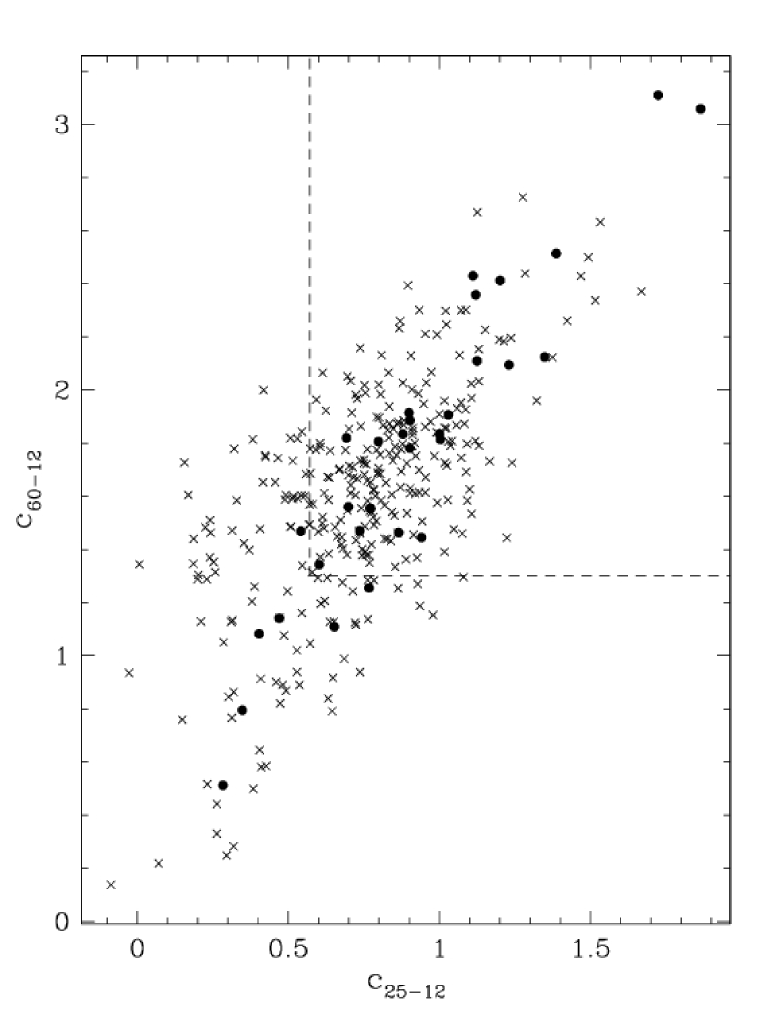
Figure 1: Colour-colour (C_a-b = log(F_a/F_b), F_a = IRAS flux in band $a$ $\mu$m) diagram of the IRAS counterparts of the sources listed in Table 1 ($\circ$), compared to that of a larger sample of H₂O masers of SFR type (a merger of Comoretto et al. com90 (1990), Brand et al. brand (1994) and Valdettaro et al. val01 (2001)) ($\times$). The dashed box defines the location of Ultracompact Hii regions (Wood & Churchwell WC89 (1989))

• the maser sources were to be of the SFR-type, i.e. associated with a SFR, to be distinguished from those associated with late-type stars. The SFR classification of Palagi et al. (PCC93 (1993)) and Valdettaro et al. (val01 (2001)) is based on IRAS colours. The location of the sources of our sample in an IRAS colour-colour plot is shown in Fig. 1 and compared with that of a much larger sample of SFRs with H₂O maser emission (a merger of Comoretto et al. com90 (1990), Brand et al. brand (1994) and Valdettaro et al. val01 (2001)). The dashed box defines the region occupied by sources with colours characteristic of ultracompact Hii regions (Wood & Churchwell WC89 (1989)). To double-check the true nature of the sources exciting the H₂O masers, other morphological indicators of the SFRs were also searched for in the literature, e.g. association with dense molecular cores (e.g Cesaroni et al. CFW98 (1999)), presence of UC Hii regions, presence of molecular outflows and other types of masers. All investigations further support the SFR identification.

• the luminosities of the associated IRAS source was to cover as large a range as possible;

• the sample was to be sufficiently large to be representative of the entire population of H₂O masers within SFRs;

• the sources were to be suitably distributed in right ascension, to avoid scheduling problems due to clustering of sources in the inner region of the Galactic plane in the large sample;

• the peak flux density was to be greater than a few Jy so that the source could be easily observed with a 5 min on-source integration time with the Medicina 32–m radio telescope;

• the number of selected sources was not to be too large to allow observations in a $<$ 2–3 day session;

• finally, in order to prevent confusion in the single beam from nearby, but unrelated, maser sources, we selected sources from the Arcetri Atlas for which no other masers had been reported within a circle of several arcminutes with single dish observations.

The main source parameters are given in Table 1, which lists:

• a running number;

• the source name;

• the associated IRAS source, when available;

• J2000.0 right ascension;

• J2000.0 declination;

• $V_{\rm cl}$, the velocity of the associated molecular cloud relative to the LSR, derived from the literature using tracers sensitive to high molecular density, such as NH₃ and CS (in km s^-1)

• $d$, the distance taken from the literature (in kpc);

• $L_{\rm IR}$, the integrated FIR luminosity (in L_⊙), usually derived from IRAS data or, otherwise, taken from the literature;

• the date of the first observation;

• references for the distance.

The IRAS luminosity was obtained by adopting the distance from Col. 7, assuming an emissivity proportional to the frequency, correcting the observed IRAS flux densities for the derived colour temperatures between two adjacent bands, and extrapolating the fluxes to 6 and 400 $\mu\mathrm{m}$ (Wouterloot et al. wou95 (1995)).

Table 1: The H₂O maser sample

#	Name	IRAS	$\alpha$(J2000)	$\delta$(J2000)	$V_{\rm cl}$	$d$	$L_{\rm IR}$	First obs.	Ref.
					(km s-1)	(kpc)	($L_{\sun}$)
1	NGC 281	00494+5617	00:52:24.7	+56:33:50	–30.8	2.2	7.9 103	01-APR-1987	1
2	W3 OH	02232+6138	02:27:04.7	+61:52:26	–46.8	2.04	6.6 104	27-MAR-1987	2
3	RNO 15–FIR	03245+3002	03:27:38.1	+30:12:59	4.7	0.35	2.0 101	30-MAR-1987	3
4	AFGL 5142	05274+3345	05:30:48.0	+33:47:54	–4.1	1.8	5.3 103	14-SEP-1995	4
5	Ori A–west	05302-0537	05:32:41.6	–05:35:47	8.9	0.5	4.0 101	13-FEB-1990	5,6
6	KL IRC2		05:35:14.5	–05:22:30	9.0	0.45	8.0 104	30-MAR-1987	6
7	OMC 2	05329-0512	05:35:27.6	–05:09:35	11.1	0.45	2.0 102	26-MAR-1987	6
8	Sh 2–231	05358+3543	05:39:12.9	+35:45:51	–17.6	2.00	6.4 103	23-MAR-1987	7
9	HHL 26	05373+2349	05:40:24.1	+23:50:55	2.0	2.4	1.8 103	09-JUL-1988	8
10	Sh 2–235	05375+3540	05:40:53.3	+35:41:49	–57.0	1.8	1.1 104	31-MAR-1987	9,34
11	NGC 2071	05445+0020	05:47:05.4	+00:21:43	9.5	0.39	4.1 102	20-MAR-1987	10
12	HH 397A	05553+1631	05:58:13.9	+16:32:00	5.7	2.0	3.0 103	20-MAR-1989	11
13	Mon R2 IRS3	06053-0622	06:07:48.0	–06:22:57	10.5	0.8	3.2 104	03-MAY-1988	12
14	Sh 2–252	06055+2039	06:08:35.5	+20:39:13	8.9	2.0	4.0 103	01-APR-1987	13
15	AFGL 5180	06058+2138	06:08:53.3	+21:38:12	3.3	1.5	5.0 103	19-DEC-1998	4
16	GGD 12–15	06084-0611	06:10:52.2	–06:11:32	11.4	1.0	7.9 103	17-JUN-1987	14
17	Sh 2–255/7	06099+1800	06:12:53.6	+17:59:27	7.0	2.5	4.7 104	22-MAR-1987	15
18	Sh 2–269	06117+1350	06:14:36.5	+13:49:35	18.2	5.3	1.2 105	22-MAR-1987	16
19	NGC 2264	06384+0932	06:41:10.1	+09:29:22	9.0	0.8	2.1 103	24-OCT-1992	17
20	G31.41+0.31	18449-0115	18:47:34.7	–01:12:46	98.0	7.9	2.6 105	22-MAR-1987	18
21	W43 Main3		18:47:47.0	–01:54:35	98.7	6.54	1.5 106	31-MAR-1987	19
22	G32.74–0.08	18487-0015	18:51:21.9	–00:12:09	38.2	2.6	5.3 103	12-JUN-1987	20
23	G34.26+0.15	18507+0110	18:53:18.8	+01:14:56	57.8	3.9	7.5 105	22-MAR-1987	20,18
24	G35.20–0.74	18556+0136	18:58:12.6	+01:40:37	34.0	1.8	1.4 104	01-APR-1987	20
25	OH43.8–0.1	19095+0930	19:11:54.2	+09:35:55	41.0	2.8	2.7 104	22-MAR-1987	21
26	G45.07+0.13	19110+1045	19:13:22.0	+10:50:52	58.5	6.0	4.4 105	01-APR-1987	18
27	G59.78+0.06	19410+2336	19:43:11.5	+23:43:54	22.3	2.2	1.5 104	01-APR-1987	22
28	ON 1	20081+3122	20:10:09.1	+31:31:37	13.0	3.0	2.7 104	23-MAR-1987	7
29	IRAS 20126+4104	20126+4104	20:14:26.0	+41:13:33	–3.6	1.7	1.0 104	21-MAR-1989	23
30	AFGL 2591	20275+4001	20:29:24.9	+40:11:20	–5.7	1.0	2.0 104	31-MAR-1987	24
31	W75–N		20:38:36.4	+42:37:35	10.0	2.0	1.4 105	22-MAR-1987	25
32	Sh 2–128(H$_2$O)	21306+5540	21:32:11.4	+55:53:55	–71.0	6.5	8.9 104	26-MAR-1987	20
33	AFGL 2789	21381+5000	21:39:58.2	+50:14:22	–43.9	5.7	4.5 104	29-JAN-1989	26
34	IC1396n	21391+5802	21:40:41.9	+58:16:12	0.0	0.62	3.2 102	21-MAR-1989	27
35	NGC 7129 FIRS2		21:43:00.2	+66:03:26	–10.1	1.0	4.3 102	26-OCT-1991	20
36	Sh 2–140 IRS1	22176+6303	22:19:18.3	+63:18:47	–7.1	0.9	2.6 104	30-MAR-1987	7
37	L1204–G	22198+6336	22:21:26.7	+63:51:38	–10.8	0.9	5.9 102	04-DEC-1989	28,7
38	IRAS 22506+5944	22506+5944	22:52:36.9	+60:00:48	–51.5	5.7	2.2 104	12-JUN-1987	29
39	Cepheus A	22543+6145	22:56:18.1	+62:01:46	–10.7	0.73	2.5 104	11-FEB-1987	30
40	WB89–234H$_2$O	23004+5642	23:02:31.8	+56:57:44	–53.5	5.6	9.6 103	17-SEP-1995	31
41	Sh 2–158	23116+6111	23:13:44.7	+61:28:10	–56.9	2.5	2.5 105	12-JUN-1987	32
42	IRAS 23139+5939	23139+5939	23:16:10.3	+59:55:29	–44.0	3.5	1.0 104	12-JUN-1987	33
43	IRAS 23151+5912	23151+5912	23:17:20.8	+59:28:47	–54.7	3.5	3.9 104	12-JUN-1987	33

Distances from: (1) Georgelin (geo75 (1975)); (2) Hachisuka et al. (hachi06 (2006)); (3) Herbig & Jones (hj83 (1983)); (4) Snell et al. (sn88 (1988)); (5) adopted distance by Fukui et al. (fukui (1986)), Meehan et al. (meeha (1998)) quote $d=0.45$ kpc; (6) adopted distance, for a recent review of distance determinations to the Orion region see Jeffries (jeff (2007)); (7) Palagi et al. (PCC93 (1993)); (8) Molinari et al. (mol02 (2002)); (9) Evans & Blair (nayo (1981)); (10) Anthony-Twarog (antw (1982)); (11) Shepherd & Churchwell (devi (1996)); (12) Racine (raci (1968)); (13) Lada & Wooden (lawo (1979)); (14) Racine & van den Bergh (ravdb (1970)); (15) Hunter & Massey (massey (1990)); (16) M. Honma, private communication; (17) Walker (walker (1956)); (18) Churchwell et al. (cwc (1990)); (19) kinematic distance, using the rotation curve of Brand & Blitz (bb93 (1993)); (20) Valdettaro et al. (VPBCCFP2002 (2002)); (21) Honma et al. (hon05 (2005)); (22) Y. Xu, private communication; (23) Wilking et al. (wilky (1989)); (24) van der Tak et al. (vdt (1999)); (25) Hunter et al. (hun94 (1994)); (26) Clarke et al. (clarke (2006)); (27) de Zeeuw et al. (deze (1999)); (28) Crampton & Fisher (cramfis (1974)); (29) Molinari et al. (mol96 (1996)); (30) Blaauw et al. (bla59 (1959)); (31) Brand & Wouterloot (bw98 (1998)); (32) L. Moscadelli, private communication; (33) Wouterloot & Walmsley (wouw (1986)); (34) Armandroff & Herbst (arma (1981)).

The sample covers a range of IR luminosities from 20 L_⊙ to $1.5\times 10^{6}$ L_⊙. These values bracket the entire luminosity interval of the regions where H₂O maser of the SFR-type are found (Palagi et al. PCC93 (1993)). In the histogram of Fig. 2 the distribution of the IR luminosities of the sources in our sample is compared with that of a much larger sample of SFR with H₂O maser emission (Palagi et al. PCC93 (1993)). Both histograms are normalized to their respective total number of sources. The small decrease of sources in our sample at large luminosities is probably due to the clustering of bright masers in the inner region of the Galactic plane which is less sampled according to criterion (4). The slightly larger percentage of sources in our sample at low luminosities is due to H₂O masers added after the publication of the Palagi et al. (PCC93 (1993)) sample.

Similarly, in Fig. 3 the distribution of H₂O maser integrated fluxes of our sources in the last observing run (February 2007) is compared with that of a much larger sample of SFR (a merger of Comoretto et al. com90 (1990), Brand et al. brand (1994) and Valdettaro et al. val01 (2001)). Both histograms are normalized to their respective total number of sources.

Figure 3 shows that in Feb. 2007 there were percentage-wise, more sources with high integrated flux densities in our present sample than there are in the comparison catalogue. Likewise there is a smaller percentage of sources with low integrated flux densities. For a large range in $L_{\rm IR}$ the general trend is for the average integrated flux density to increase with increasing $L_{\rm IR}$ (e.g., Brand et al. (BCCFPPV2003 (2003)); this trend will be further investigated in a forthcoming paper) and the difference between the distributions shown in Fig. 3 reflects the fact that we have biased our present sample towards sources of high $L_{\rm IR}$, in order to have a good chance of yielding a maser detection in a reasonable amount of integration time. On the other hand, sources of lower $L_{\rm IR}$ usually have a lower flux density, and do not have a 100% detection rate (e.g., Brand et al. brand2007 (2007)). This, in combination with our present sample’s bias towards sources with higher $L_{\rm IR}$ can be seen as the main cause of the difference between the histograms in Fig. 3 for the lower integrated flux density bins. Furthermore, on the low flux density side, the difference between the histograms is enhanced by the way sources from the comparison catalogue were counted (if there was more than one observation, we always selected the one in which the source was detected). Note that although in Fig. 3 we show the distribution of integrated flux densities for the observing session of Feb. 2007, any other session would have given the same statistical result. In summary and within the limitations inherent in the comparison, we confirm that our sample is fairly representative of the entire population of SFRs.

Ideally, from the observed maser variability, we would like to infer the properties of the exciting YSO and of its surroundings. However, while for H₂O masers from late–type stars the association is unambiguous (i.e. there is only one star pumping the maser), for SFR-type masers, several distinct YSOs may simultaneously be present within our beam. This ambiguity can only be solved with high–resolution interferometric observations, but even if in many cases these are available, they cover at most a few epochs and there is no guarantee that the spatial/velocity situation of the maser spots remains the same over long time intervals, given the large variability observed.

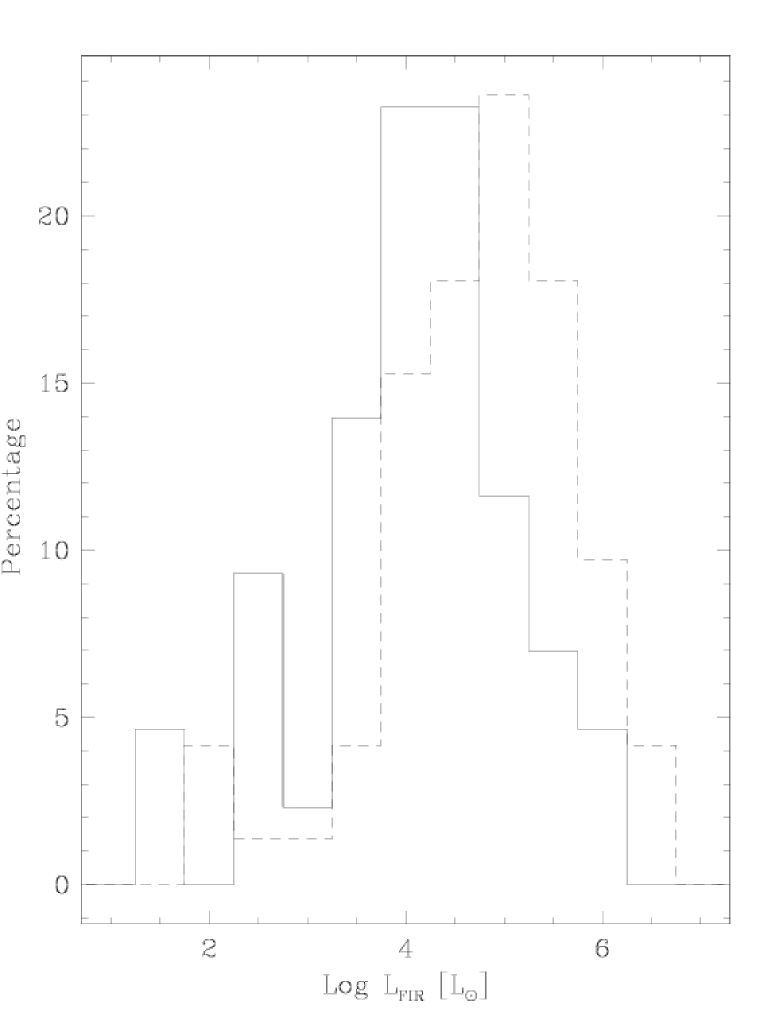
Figure 2: The distribution of IR luminosity of the SFRs in our sample (solid line) and that of a larger sample of SFRs (Palagi et al. PCC93 (1993)) (dashed line). Both histograms are normalized to the total number of sources.

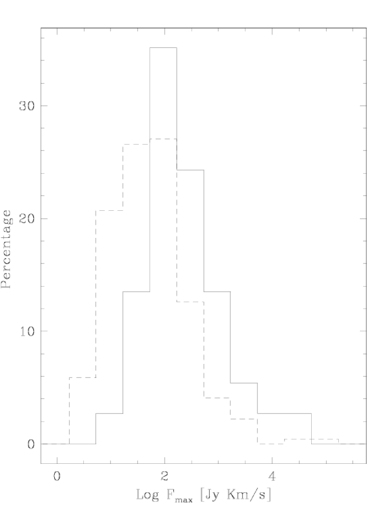
Figure 3: The distribution of the integrated fluxes of the H₂O masers in our sample as measured in the Feb. 2007 observing session (solid line), and that of a larger sample of SFRs (a merger of Comoretto et al. com90 (1990), Brand et al. brand (1994) and Valdettaro et al. val01 (2001)) (dashed line).

3 Observations

The present study is based on observations carried out with the Medicina 32–m radiotelescope (HPBW $\sim$1.^′9 at 22 GHz). This is primarily set up to be used for VLBI measurements, and therefore the front-end is optimized for such work.

The monitoring program is ongoing but the time interval considered in this work spans 20 years, from March 1987 to February 2007, with shorter time coverage for a few sources which were added to the list at a later date. During this period, various parts of the whole system (antenna, receiver, autocorrelator) were improved, increasing the sensitivity and spectral resolution of the observations. A detailed description of the system and its improvements can be found in Comoretto et al. (com90 (1990)) and in Brand et al. (brand (1994)), respectively. In 1989 realigning of the antenna surface resulted in an improvement of the efficiency at 22 GHz from 17 to 38%. The original backend was a 512-channel digital autocorrelator; in 1991 the number of channels was increased to 1024. In the same year a HEMT amplifier replaced the GaAs FET front-end, reducing the system temperature. In 1991 an active sub-reflector control increased the gain at low and high elevations.

The available bandwidth varied between 3.125 MHz and 25 MHz (at 22 GHz this corresponds to a velocity resolution between 0.041 km s^-1 and 0.658 km s^-1). In February 1997, the VLA-1 chip correlator was replaced by a new one based on the NFRA correlator chips and boards (Bos bos (1991)). The new autocorrelator has 2048 delay channels and 160 MHz maximum bandwidth in its standard configuration. In order to maintain compatibility with previous observations, we have continued to use only 1024 channels and a 10 MHz bandwidth, giving a velocity resolution of 0.132 km s^-1. Finally, owing to extensive maintenance works on the radiotelescope, there is a gap in the observations from April 1996 to February 1997.

The telescope pointing model is typically updated a few times per year, and is quickly checked every few weeks by observing strong maser sources (e.g., W3 OH, Orion-KL, W49 N, Sgr B2 and W51). The pointing accuracy was always better than 25″; from about mid-2004 the rms residuals from the pointing model were about 8″–10″.

Observations were taken in position-switching mode, with both ON and OFF scans of 5 min duration. The OFF position was taken 1.25° E of the source position to rescan the same path as the ON scan. Typically, one ON/OFF pair was taken, though for weak sources this was repeated several times. The typical 1 $\sigma$ noise-level in the spectra is $\sim$1.5 Jy.

3.1 Calibration

The calibration of the intensities and the velocities is one of the main concerns for variability studies.

The antenna gain as a function of elevation is determined by daily observations of the continuum source DR 21 (for which we assume a flux density of 16.4 Jy after scaling the value of 17.04 Jy given by Ott et al. ott (1994) for the ratio of the source size to the Medicina beam) at a range of elevations. Antenna temperatures were derived from total power measurements in position switching mode. Integration time in each position is 10 sec with 400 MHz bandwidth. The zenith system temperature is about 120 K in clear weather conditions.

The daily gain curve was determined by fitting a polynomial curve to the data, which was then used to convert antenna temperature to flux density for all spectra taken that day. From the dispersion of the single measurements around the curve we find the typical calibration uncertainty to be 19%. On the few days for which no separate gain curve was measured, we applied that which was closest in time, and estimated a corresponding calibration uncertainty of 7%. The average overall calibration uncertainty is therefore estimated to be $\sim$20%.

To reduce the effects of atmospheric attenuation variations, observations were obtained in good weather conditions and at elevations $\geq$ 30^∘, or around source meridian transit for low declination sources. For several sources we compared our intensities with those available in the literature and close in time with our observations, virtually always finding very good agreement within the above-quoted uncertainty (e.g., Valdettaro et al. VPBCCFP2002 (2002)). A good agreement was also found comparing observations taken at Effelsberg in a program to study H₂O masers associated with late–type stars which was run jointly by the Medicina and Effelsberg radiotelescopes.

As for the calibration of the velocity scale and its stability over time, checks were made with quasi simultaneous Effelsberg observations showing a good agreement. However, it is difficult to quote a definite uncertainty considering the variable nature of the sources and the not simultaneous observations. To make sure that the velocity changes that will be reported are real effects and not due to instrumental changes (e.g., local oscillator drifts in our system) and to evaluate the uncertainty, we performed internal consistency checks within the sources of our sample. The source G32.74-0.08 is characterized by a single, narrow and intense velocity component. The observed velocity of the peak of the emission displays a maximum deviation from a linear fit over the entire period of $<$ 0.1 km s^-1, a value that will be used as maximum possible uncertainty on the velocity throughout our patrol.

4 The database

For the purposes of the present study, the standard reduction procedures were applied to the observed spectra before including them in the database:

• the edges of the available band were deleted to limit the spectra to the flatter part of the band. This means that the velocity coverage shown may be smaller (generally by 20-30%) than the nominal bandwidth of the autocorrelator;

• the spectra taken within 10 days were averaged, unless a significant difference was found;

• a polynomial fit to the channels free of line emission was removed from the spectra;

• rebinning to 0.3 km s^-1 was applied.

The whole set of Medicina 32–m observations is archived in CLASS format. The raw data can be accessed through contact with the authors.

The amount of information present in the database is so large that a concise way of presentation is essential for a rapid visual appreciation of the properties of maser variability. Below we describe our selection. All plots and figures presented can be found in electronic form in the online appendix.

4.1 The spectra

The most obvious presentation is a time sequence of spectra. These are arranged in a compact form as page-plots in which each page contains 18 spectra, with time running from top to bottom and from left to right. In each spectrum, the date of observation is reported in the top left corner, and the number of days elapsed since the first observation of the source is shown in the top right corner. The velocity scale is the same for all spectra of each source and is bracketed by the minimum and maximum velocities at which emission has been detected (above the 5 $\sigma$ level) throughout the monitoring period. Given the large range of intensities present during our patrol, we present the spectra using an autoscaled flux density scale. These plots are convenient to view the full details of each spectrum except for those with bursts, although they have the disadvantage that the flux density scale changes from spectrum to spectrum and the visual impression of the variability is lost.

As an example we show in Fig. 4 the first page of the spectra for the source W75–N.

The following two additional presentations of the spectra can be downloaded from our WEB pages.

• Fixed–linear flux density scale, where the maximum flux density is determined by the maximum value observed during our monitoring. These plots are convenient for a quick estimate of the variability, but compress the spectra too much when the source presents bursts with intensities orders of magnitude larger than the “quiescent” value.

• Same as in (1) but with logarithmic flux density scale. The minimum flux density is equal to the 5 $\sigma$ level in each spectrum.

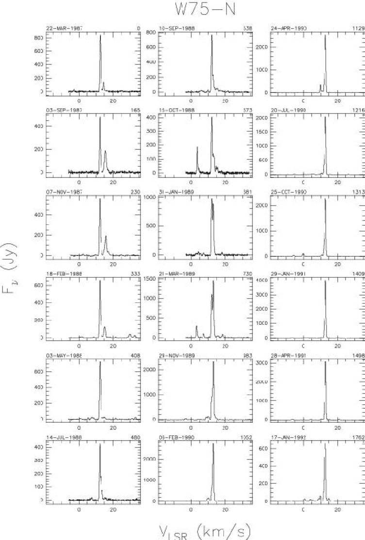
Figure 4: The first 18 spectra of the source W75–N with an autoscaled flux density scale. Time runs from top to bottom and from left to right. In each spectrum the actual date of observation is given above the top left corner, and the number of days elapsed since the first observation of the source above the top right corner. The velocity scale is the same for all spectra.

4.2 The velocity–time–flux density plots

A more concise visualization of the time variation of the maser emission can be obtained by showing the flux density versus velocity and time in the same diagram.

Since the observed dates are not distributed evenly in time, some kind of interpolation between two adjacent observations must be used. As no assumption can be made on the evolution of the H₂O maser components, we chose a linear interpolation. This procedure produces an apparent increase in the lifetime of a feature when long time-intervals between two consecutive observations occur.

Two versions of these plots are presented:

• full plots, with velocity coverage extending to the maximum velocity covered during the observations;

• zoomed plots, with velocity coverage limited to the part of the spectrum where emission has been detected (above the 5 $\sigma$ level) at least once during the patrol.

In these plots, only emission above the 5 $\sigma$ level is shown. In both plots the vertical solid line indicates the velocity of the thermal molecular gas (either CO, CS or NH₃). In the zoomed plots the additional dashed line represents the mean velocity derived from the histogram of the rate–of–occurrence (see Sect. 4.5). The time-scale on the left is in days starting from the first observation. To convert this scale to real dates one should use the date given in the first spectrum of the figure with the time sequence of spectra, e.g., Fig. 4 for W75–N or the date listed in Table 1. These plots are particularly useful to find possible velocity drifts and to separate steady components from bursts of short duration.

As an example of the velocity–time–flux density full and zoomed plots, in Fig. 5–6 we show those of the source W75–N.

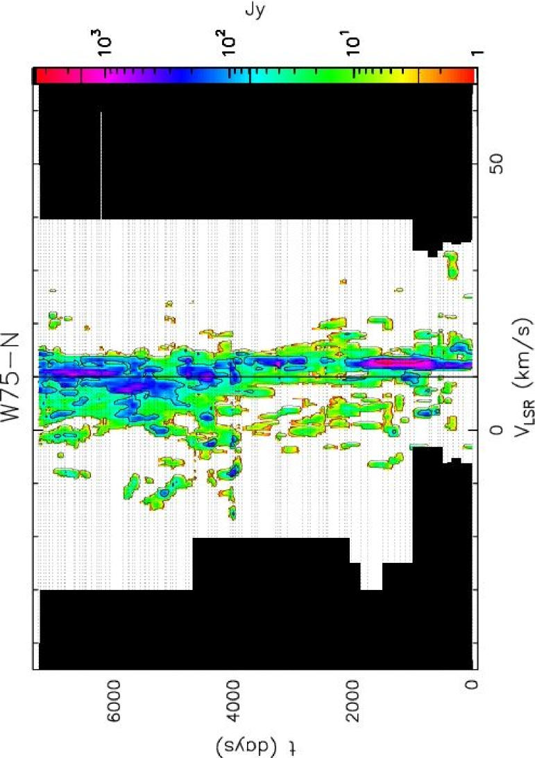
Figure 5: The velocity–time–flux density full plot of the source W75–N. The vertical solid line indicates the velocity of the associated thermal molecular gas. The flux density scale is shown by the bar on the right. In this bar the three lines give the flux density of the drawn contours. The area in black indicates that the corresponding velocity range was not observed. (This figure is in colour both in the electronic edition and in the online appendix.)

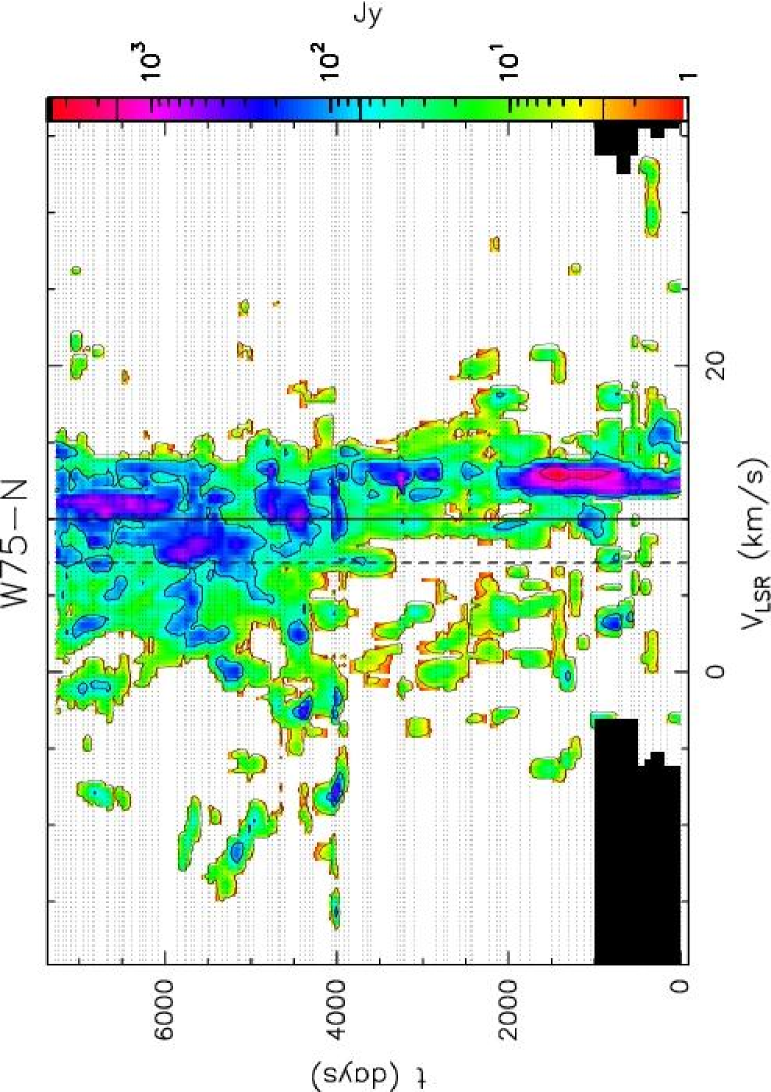
Figure 6: The velocity–time–flux density zoomed plot of the source W75–N. The vertical solid line indicates the velocity of the associated thermal molecular gas. The vertical dashed line marks the mean velocity derived from the histogram of the rate–of–occurrence. The flux density scale is shown by the bar on the right. In this bar the three lines give the flux density of the drawn contours. The area in black indicates that the corresponding velocity range was not observed. (This figure is in colour both in the electronic edition and in the online appendix.)

4.3 The light curve of the maser emission

A plot of the peak flux density as a function of time is often used to study the temporal behaviour of the maser emission. However, the peak flux density is meaningful only if one narrow component is present throughout the entire observing period. It has less physical meaning for complex spectra with multiple components of comparable flux densities varying in an uncorrelated fashion. In this case, the integrated flux density can only be used with the understanding that this represents the contribution of all components and may be representative of the energy input from the YSOs. However, since each velocity component may vary independently, the relative contribution of each to the light curve is lost in this plot.

An example of the light curve of the integrated flux density for the source W75–N is shown in Fig. 7.

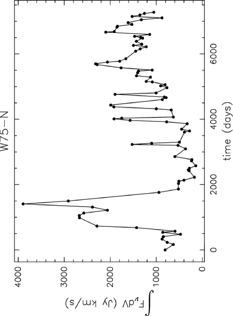
Figure 7: The integral of the flux density over the observed velocity range as a function of time for the source W75–N.

4.4 The upper and lower envelopes and the mean spectrum

Another meaningful description of the degree of maser variability is given by the comparison between the upper and lower envelopes and the mean spectra of the sources over the whole period of observation.

The upper envelope corresponds to the maximum flux density ever reached at each velocity and is obtained by finding the maximum flux density in each velocity bin. Its integral and the derived luminosity, $L_{\rm H_{2}O}$(up), represent the maximum emission that could be produced by the source if all the velocity components were to emit at their maximum level and at the same time.

The mean spectrum represents the mean flux density at each velocity, and is obtained by computing the arithmetic mean of the flux densities in each velocity bin, assigning the same weight to the individual spectra. In this average the flux density is arbitrarily set to zero if it is below the 5 $\sigma$ noise level in the spectrum in question. Clearly, the steadier components dominate this spectrum.

Finally, the lower envelope identifies the components that are always active and is obtained by finding the minimum flux density in each velocity bin, again setting it to zero if it is below the 5 $\sigma$ noise level in each spectrum. When the lower envelope is zero over the whole velocity interval, it indicates that no velocity component is constantly present above a 5 $\sigma$ level during the monitoring period. This does not necessarily imply that the maser is quiescent at all velocities at some epoch, since the emission may occur at different velocities at different times.

An example of the upper and lower envelopes, and mean spectrum of the source W75–N is shown in Fig. 8.

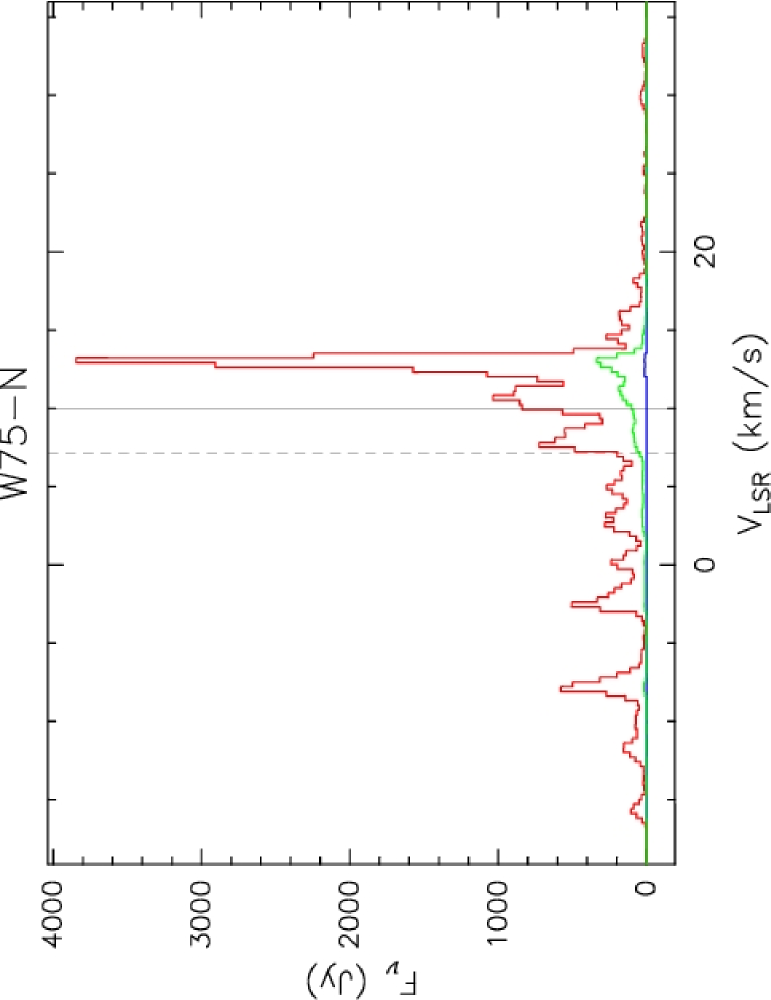
Figure 8: The upper (red) and lower (blue) envelopes and the mean spectrum (green) of the source W75–N measured during our monitoring. The vertical solid line marks the velocity of the associated thermal molecular gas. The vertical dashed line marks the mean velocity derived from the histogram of the rate–of–occurrence. (This figure is in colour both in the electronic edition and in the online appendix.)

4.5 The rate–of–occurrence plots

To identify the velocity components which are more frequently present in the spectra (independently of their flux density), we plot the rate–of–occurrence of maser emission above the 5 $\sigma$ noise level as a function of velocity. To produce this plot we have set a counter for each channel that increases by one unit every time the flux density in the channel is greater than the 5$\sigma$ noise level of the spectrum.

An example of the rate–of–occurrence histogram of the source W75–N is shown in Fig. 9.

Two histograms can be produced:

• the percentage of detections with respect to the total number of observations (dotted line histogram, scale to the right);

• the number of detections (solid line histogram, scale to the left).

The two histograms may differ slightly in velocity ranges where the time coverage is not equal for all channels, produced by using different bandwidths during our monitoring. From this histogram we can derive the mean velocity which is shown in Figs. 6 and 8.

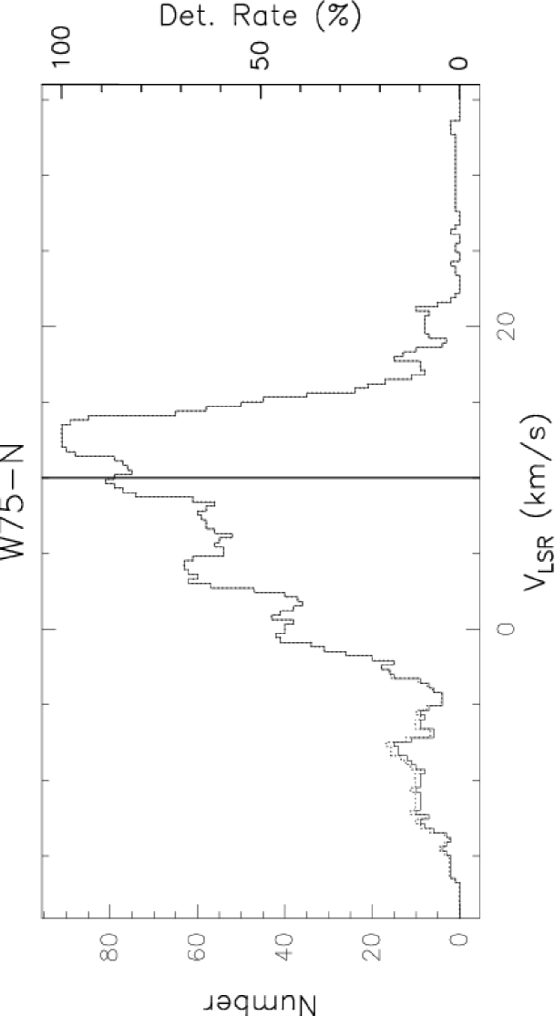
Figure 9: The rate–of–occurrence plot for the source W75–N. The scale to the right refers to the dotted histogram, the scale to the left to the solid line histogram. The vertical solid line marks the velocity of the associated thermal molecular gas.

5 Conclusions

We present the observational results of a systematic study extending for almost 20 years of the H₂O maser variability in 43 SFRs with luminosities of the associated IR sources between 20 and 1.5$\times 10^{6}$ L_⊙. This database provides the backbone for the discussion of the main long-term properties of maser emission that will be presented in a forthcoming paper. We have identified several ways to describe graphically the main aspects of the H₂O maser emission. These include:

• the spectra in a compressed form, with an autoscaled flux density scales (the same sets of plots, but with fixed linear and logarithmic flux density scales, are also available from our WEB pages);

• the velocity–time–flux density plots, which conveniently describe the morphology of the variability of the maser emission. These diagrams are particularly useful for recognizing the presence of possible velocity drifts and separating steady components from bursts of short duration;

• the velocity–integrated flux density as a function of time. This light curve describes the overall emission of the maser components associated with a SFR;

• the mean spectrum;

• the upper and lower envelopes of the maser emission. The upper envelope represents the maximum emission that the SFR could produce if all the velocity components were present simultaneously and emitting at their maximum rate. Similarly, the lower envelope pinpoints the steady components and their lowest level (but $>5\sigma$) of emission;

• the number of times that the maser emission is well above the noise ($>5\sigma$) as a function of velocity is directly gauged by the histogram of the rate–of–occurrence.

- (1) Anthony–Twarog, B. J. 1982, AJ, 87, 1213
- (2) Armandroff, T. E., & Herbst, W. 1981, AJ, 86, 1923
- (3) Blaauw, A., Hiltner, W. A., & Johnson, H. L. 1959, ApJ, 130, 69
- (4) Bos, A. 1991, IEEE Trans. on Instrumentation and Measurements, 40, 591
- (5) Brand, J., & Blitz, L. 1993, A&A, 275, 67
- (6) Brand, J., Cesaroni, R., Caselli, P., et al. 1994, A&AS, 103, 541
- (7) Brand, J., & Wouterloot, J. G. A. 1998, A&A, 337, 539
- (8) Brand, J., Cesaroni, R., Comoretto, G., et al. 2003, A&A, 407, 573
- (9) Brand, J., Felli, M., Cesaroni, R., et al. 2007, in Astrophysical Masers and Their Environments, Proceedings of IAU Symposium No 242, ed. J. Chapman, & W. A. Baan, in Press
- (10) Cesaroni, R., Palagi, F., Felli, M., et al. 1988, A&AS, 76, 445
- (11) Cesaroni, R., Felli, M., & Walmsley, C. M. 1999, A&AS, 136, 333
- (12) Churchwell, E., Walmsley, C. M., & Cesaroni, R. 1990, A&AS, 83, 119
- (13) Clarke, A. J., Lumsden, S. L., Oudmaijer, R. D., et al. 2006, A&A, 457, 183
- (14) Claussen, M. J., Wilking, B. A., Benson, P. J., et al. 1996, ApJS, 106, 111
- (15) Codella, C., Felli, M., Natale, V., Palagi, F., & Palla, F. 1994, A&A, 291, 261
- (16) Codella, C., & Felli, M. 1995, A&A, 302, 521
- (17) Codella, C., & Palla, F. 1995, A&A, 302, 528
- (18) Codella, C., Felli, M., & Natale, V. 1996, A&A, 311, 971
- (19) Comoretto, G., Palagi, F., Cesaroni, R., et al. 1990, A&AS, 84, 179
- (20) Crampton, D., & Fisher, W. A. 1974, Pub. Dom. Astrophys. Obs., 14, 283
- (21) Dent, W. A. 1972, ApJ, 177, 93
- (22) de Zeeuw, P. T., Hoogerwerf, R., de Bruijne, J. H. J., Brown, A. G. A., & Blaauw, A. 1999, AJ, 117, 354
- (23) Evans, N. J., & Blair, G. N. 1981, ApJ, 246, 394
- (24) Felli, M., Palagi, F., & Tofani, G. 1992, A&A, 255, 293
- (25) Felli, M., Massi, F., Robberto, M., & Cesaroni, R. 2006, A&A, 453, 911
- (26) Forster, J. R., & Caswell, J. L. 1989, A&A, 213, 339
- (27) Forster, J. R., & Caswell, J. L. 1999, A&AS, 137, 43
- (28) Fukui, Y., Sugitani, K., Takaba, H., et al. 1986, ApJ, 311, L85
- (29) Furuya, R. S., Kitamura, Y., Wootten, A., Claussen, M. J., & Kawabe, R. 2003, ApJS, 144, 71 (Erratum: 2007, ApJS, 171, 349)
- (30) Georgelin, Y. 1975, Thèse de Doctorat, Université de Provence
- (31) Hachisuka, K., Brunthaler, A., Menten, K. M., et al. 2006, ApJ, 645, 337
- (32) Herbig, G. H., & Jones, B. F. 1983, AJ, 88, 1040
- (33) Honma, M., Bushimata, T., Choi, Y. K., et al. 2005, PASJ, 57, 595
- (34) Hunter, D. A., & Massey, P. 1990, AJ, 99, 846
- (35) Hunter, T. R., Taylor, G. B., Felli, M., & Tofani, G. 1994, A&A, 284, 215
- (36) Jeffries, R. D. 2007, MNRAS, 376, 1109
- (37) Lada, C. J., & Wooden, D. 1979, ApJ, 232, 158
- (38) Liljeström, T., Mattila, K., Toriseva, M., & Anttila, R. 1989, A&AS, 79, 19
- (39) Little L. T., White, G. J., & Riley, P. W. 1977, MNRAS, 180, 639
- (40) Meehan, L. S. G., Wilking, B. A., Claussen, M. J., Mundy, L. G., & Wootten, A. 1998, AJ, 115, 1599
- (41) Molinari, S., Brand, J., Cesaroni, R., & Palla, F. 1996, A&A, 308, 573
- (42) Molinari, S., Testi, L., Rodríguez, L. F., & Zhang, Q. 2002, ApJ, 570, 758
- (43) Ott, M., Witzel, A., Quirrenbach, A., et al. 1994, A&A, 284, 331
- (44) Palagi, F., Cesaroni, R., Comoretto, G., Felli, M., & Natale, V. 1993, A&AS, 101, 153
- (45) Palla, F., Brand, J., Comoretto, G., Felli, M., & Cesaroni, R. 1991, A&A, 246, 249
- (46) Palla, F., Cesaroni, R., Brand, J., et al. 1993, A&A, 280, 599
- (47) Persi, P., Palagi, F., & Felli, M. 1994, A&A, 291, 577
- (48) Racine, R. 1968, AJ, 73, 233
- (49) Racine, R., & van den Bergh, S. 1970, Reflection Nebulae and Spiral Structure, in The Spiral Structure of our Galaxy, ed. W. Becker, & G. I. Kontopoulos (Dordrecht: Reidel), IAU Symp. 38, 219
- (50) Rudnitskij, G. M., Paschenko, M. I., Lekht, E. E., et al. 2007, in Astrophysical Masers and Their Environments, Proceedings of IAU Symposium No 242, ed. J. Chapman, & W. A. Baan, in Press
- (51) Shepherd, D. S., & Churchwell, E. 1996, ApJ, 472, 225
- (52) Snell, R. L., Huang, Y.-L., Dickman, R. L., & Claussen, M. J. 1988, ApJ, 325, 853
- (53) Tofani, G., Felli, M., Taylor, G. B., & Hunter, T. R. 1995, A&AS, 112, 299
- (54) Valdettaro, R., Palla, F., Brand, J., et al. 2001, A&A, 368, 845
- (55) Valdettaro, R., Palla, F., Brand, J., et al. 2002, A&A, 383, 244
- (56) van der Tak, F. F. S., van Dishoeck, E. F., Evans, N. J., Bakker, E. J., & Blake, G. A. 1999, ApJ, 522, 991
- (57) Walker, M. F. 1956, ApJS, 2, 365
- (58) Wilking, B. A., Blackwell, J. H., Mundy, L. G., & Howe, J. E. 1989, ApJ, 345, 257
- (59) Wood, D. O. S., & Churchwell, E. 1989, ApJ, 340, 265
- (60) Wouterloot, J. G. A., & Walmsley, C. M. 1986, A&A, 168, 237
- (61) Wouterloot, J. G. A., Fiegle, K., Brand, J., & Winewisser, G. 1995, A&A, 301, 236 (Erratum: 1997, A&A, 319, 360)