Mapping Cartesian Coordinates into Emission Coordinates: some Toy Models

Abstract

After briefly reviewing the relativistic approach to positioning systems based on the introduction of the emission coordinates, we show how explicit maps can be obtained between the Cartesian coordinates and the emission coordinates, for suitably chosen set of emitters, whose world-lines are supposed to be known by the users. We consider Minkowski space-time and the space-time where a small inhomogeineity is introduced (i.e. a small ”gravitational” field), both in 1+1 and 1+3 dimensions.

I Introduction

The current positioning systems, such as GPS, are based on a classical space and an absolute time, over which some relativistic corrections are added, in order to take into account the effects arising from both the Special and General Theory of Relativity (see ashby1 ; ashby2 and references therein). A new approach to the problem of positioning has been proposed by B. Collcollsypor , which introduces a shift from the Newtonian viewpoint to a true relativistic framework, where a new and operational definition of space-time coordinates is given.

The starting assumption in the construction of such a new system of coordinates is that an ideal electromagnetic signal propagates along a null geodesic. Indeed, the main idea can be summarized as follows: let us consider 4 clocks, moving along arbitrary world-lines in space-time, and broadcasting their proper times, by means of electromagnetic signals. Then, any observer, at a given space-time point $P$ along his own world-line, receives 4 numbers, carried by the 4 signals emitted by the clocks. These 4 numbers, say $\tau_{1},\tau_{2},\tau_{3},\tau_{4}$, are nothing but the proper times of the emitting clocks and constitute the coordinates of that space-time point; they are usually referred to as emission coordinates collem ; ferrando . In other words, the past light cone of a space-time point $P$ cuts the clocks world-lines at 4 points, and the proper times measured along the clocks world-lines, are the coordinates of $P$. In practice, the clocks are supposed to be carried by satellites (which, in what follows, are referred to also as emitters) orbiting the Earth, and the observers are the users on the Earth, or on board of other satellites also.

Actually, a 2-dimensional approach to this new paradigm of relativistic positioning has been thoroughly described by Coll and collaborators coll1a ; coll2a : there, the definition of the coordinates domain (i.e. the space-time region where emission coordinates are well defined), the information that the data coming from a relativistic positioning system give on the space-time metric interval and the interest of these results in gravimetry, are discussed and analyzed for some prototypical situations.

In this paper, starting from the results obtained in coll1a ; coll2a , we show how an explicit map can be obtained from the Cartesian coordinates and the emission coordinates, for suitably chosen set of emitters, whose world-lines are supposed to be known by the users. We start from the 2-dimensional cases, both in inertial and accelerated frames, and show how the results can be generalized to 4-dimensional cases, in order to deal with Minkowski 1+3 dimensional space-time and the space-time where a small inhomogeneity is introduced (i.e. a small ”gravitational” field).

II Emission coordinates in 1+1 dimensional space-time

In this Section, we briefly review how emission coordinates can be introduced in a 1+1 dimensional space-time, according to the approach outlined in coll1a .

The simplified system we are dealing with is composed of (i) two emitters, whose world-lines are $\gamma_{1}$, $\gamma_{2}$; they broadcast to the users their proper times $\tau^{1},$ $\tau^{2}$ and, also, the proper times $\overline{\tau}^{2}$, $\overline{\tau}^{1}$ that they receive each one from the other; (ii) a generic user, whose world-line is $\gamma$. The user is supposed to be in $\Omega$, which is the region of space-time where the emission coordinates are properly defined; in the situation we are considering, $\Omega$, which is called coordinate domain, is the space-time region between the world-lines of the two emitters (see figure 1). The user, is supposed to receive the four broadcasted times $\{\tau^{1},\tau^{2};\overline{\tau}^{1},\overline{\tau}^{2}\}$. We recall that the set of these proper times allows the user to determine the equation of his trajectory $\tau^{2}=F(\tau^{1}),$ and, also, the trajectories of the emitters $\varphi_{1}(\tau^{1})=\overline{\tau}^{2}$, $\varphi_{2}(\tau^{2})=\overline{\tau}^{1}$.

Now, we suppose to know the world-lines of the emitters in a suitable system of null coordinates $\{u,v\}$. We remember (see, for instance coll1a ) that, in such a coordinate system, the space-time metric has the form.

$$ds^{2}=m(u,v)dudv.$$ (1)

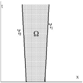
Figure 1: The two emitters move along the world-lines $\gamma_{1},\gamma_{2}$, and every event in the domain $\Omega$ between both emitters can be unambiguously labelled by the proper times $(\tau^{1},\tau^{2})$.

The world-lines of the emitters, in terms of their proper times, are given by the following expressions:

$$\gamma_{1}\equiv\begin{cases}{u}=u_{1}(\tau^{1})\\ {v}=v_{1}(\tau^{1})\end{cases}\qquad\gamma_{2}\equiv\begin{cases}{u}=u_{2}(\tau^{2})\\ {v}=v_{2}(\tau^{2})\end{cases}.$$ (2)

Then, the emission coordinates $\{\tau^{1},\tau^{2}\}$ are defined by the following change of variables from the null coordinates $\{{u},{v}\}$:

$$\begin{array}[]{l}{u}=u_{1}(\tau^{1})\\ {v}=v_{2}(\tau^{2})\end{array}\Rightarrow\begin{array}[]{l}\tau^{1}=u_{1}^{-1}({u})=\tau^{1}({u})\\ \tau^{2}=v_{2}^{-1}({v})=\tau^{2}({v}).\end{array}$$ (3)

Consequently, the emitter world-lines (2) can be expressed in emission coordinates, and they have the following expression:

$$\gamma_{1}\equiv\begin{cases}\tau^{1}=\tau^{1}\\ \tau^{2}=\varphi_{1}(\tau^{1})\doteq\overline{\tau}^{2}\end{cases}\qquad\gamma_{2}\equiv\begin{cases}\tau^{1}=\varphi_{2}(\tau^{2})\doteq\overline{\tau}^{1}\\ \tau^{2}=\tau^{2}\end{cases}$$ (4)

where the functions $\varphi_{1}(\tau^{1})$, $\varphi_{2}(\tau^{2})$ are determined on considering that the events along the two world-lines are connected by coordinate lines $v=const$ and $u=const$ (see below). We remember also that, in terms of the emission coordinates, we may write the metric in the form (thanks to the change of coordinates (3)):

$$\begin{array}[]{c}ds^{2}=m(\tau^{1},\tau^{2})d\tau^{1}d\tau^{2}\\[11.38109pt] m(\tau^{1},\tau^{2})={m}(u_{1}(\tau^{1}),v_{2}(\tau^{2}))u_{1}^{\prime}(\tau^{1})v_{2}^{\prime}(\tau^{2}).\end{array}$$ (5)

III Emission coordinates for inertial emitters in Minkowski space-time

Figure 2: (a) The events corresponding to proper times $\tau^{1}$ along the world-line $\gamma_{1}$ and $\overline{\tau}^{2}$ along the world-line $\gamma_{2}$ are connected by a coordinate line $v=const$ and, hence, they have the same coordinate $v$; similarly, the events corresponding to proper times $\tau^{2}$ along the world-line $\gamma_{2}$ and $\overline{\tau}^{1}$ along the world-line $\gamma_{1}$ are connected by a coordinate line $u=const$ and, hence, they have the same coordinate $u$. (b) The positioning data received at $P$ by the user, thanks to the properties of the coordinate lines, allow to establish that $u_{1}(\overline{\tau}^{1}_{P})=u_{2}({\tau}^{2}_{P})$, $v_{1}({\tau}^{1}_{P})=v_{2}(\overline{\tau}^{2}_{P})$, and similarly for positioning data received at $Q$: $u_{1}(\overline{\tau}^{1}_{Q})=u_{2}({\tau}^{2}_{Q})$, $v_{1}({\tau}^{1}_{Q})=v_{2}(\overline{\tau}^{2}_{Q})$

As an example of what we have outlined above, we show how to build emission coordinates for a set of two emitters, moving with constant velocity $v_{i},\ i=1,2$ in Minkowski 1+1 dimensional space-time.

To begin with, we write their world-lines in null coordinates, as functions of the proper times $\tau^{1},\tau^{2}$:

$$\gamma_{1}\equiv\begin{cases}\,{u}=\lambda_{1}\tau^{1}\\[2.84526pt] \,{v}=\displaystyle\frac{1}{\lambda_{1}}\tau^{1}+v_{0}\end{cases}\ \gamma_{2}\equiv\begin{cases}\,{u}=\lambda_{2}\tau^{2}+u_{0}\\[2.84526pt] \,{v}=\displaystyle\frac{1}{\lambda_{2}}\tau^{2}\end{cases},$$ (6)

where $\lambda_{i}\doteq\sqrt{\frac{1+v_{i}}{1-v_{i}}},\quad i=1,2$ are the shift functions of the two emitters (see coll1a ).

Then, the emission coordinates are defined by:

$$\begin{array}[]{lll}{u}=u_{1}(\tau^{1})=\lambda_{1}\tau^{1}&\Rightarrow&\tau^{1}=\displaystyle\frac{1}{\lambda_{1}}\,{u}\\[5.69054pt] {v}=v_{2}(\tau^{2})=\displaystyle\frac{1}{\lambda_{2}}\tau^{2}&\Rightarrow&\tau^{2}=\lambda_{2}{v}.\end{array}$$ (7)

Furthermore, on applying (5), we can easily obtain the metric tensor in emission coordinates (in the case of a straight line it is $m\left(u,v\right)=1$):

$$m(\tau^{1},\tau^{2})=u_{1}^{\prime}(\tau^{1})v_{2}^{\prime}(\tau^{2})=\frac{\lambda_{1}}{\lambda_{2}},$$ (8)

and the space-interval turns out to be

$$ds^{2}=\lambda\,d\tau^{1}d\tau^{2}\,,\qquad\lambda\equiv\frac{\lambda_{1}}{\lambda_{2}}.$$ (9)

Now, let us work out how to express the emitters world-lines in emission coordinates. As we wrote before, this can be done if we admit that the emitters broadcast their proper times $\overline{\tau}^{2}$, $\overline{\tau}^{1}$ to each other. Then, the functions $\varphi_{1}(\tau^{1})$, $\varphi_{2}(\tau^{2})$ are determined by considering that the events corresponding to proper times $\tau^{1}$ along the world-line $\gamma_{1}$ and $\overline{\tau}^{2}$ along the world-line $\gamma_{2}$ are connected by a coordinate line $v=const$, similarly for the the events corresponding to proper times $\tau^{2}$ along the world-line $\gamma_{2}$ and $\overline{\tau}^{1}$ along the world-line $\gamma_{1}$ (see figure 2a).

Consequently, the emitters world-lines in emission coordinates are

$$\gamma_{1}\equiv\begin{cases}\tau^{1}=\tau^{1}\\ \tau^{2}=\varphi_{1}(\tau^{1})\equiv\displaystyle\frac{1}{\lambda}\tau^{1}+\tau^{2}_{0}\end{cases}$$ (10)

$$\gamma_{2}\equiv\begin{cases}\tau^{1}=\varphi_{2}(\tau^{2})\equiv\displaystyle\frac{1}{\lambda}\tau^{2}+\tau^{1}_{0}\\ \tau^{2}=\tau^{2}.\end{cases}$$ (11)

Let us now consider the set of positioning data $\left({\tau}^{1}_{P},{\tau}^{2}_{P},\overline{\tau}^{1}_{P},\overline{\tau}^{2}_{P}\right)$, $\left({\tau}^{1}_{Q},{\tau}^{2}_{Q},\overline{\tau}^{1}_{Q},\overline{\tau}^{2}_{Q}\right)$ received by the user at the events $P$ and $Q$, respectively. Due to the fact that the corresponding emission events are connected by coordinate lines $u=const$ or $v=const$, it is possible to show that

$$\frac{\Delta\tau^{1}\Delta\tau^{2}}{\Delta\overline{\tau}^{1}\Delta\overline{\tau}^{2}}=\frac{\lambda_{1}^{2}}{\lambda_{2}^{2}}=\lambda^{2},$$ (12)

where $\Delta\tau^{1}\doteq\tau^{1}_{Q}-\tau^{1}_{P},\quad\Delta\tau^{2}\doteq\tau^{2}_{Q}-\tau^{2}_{P}\quad$, $\Delta\overline{\tau}^{1}\doteq\overline{\tau}^{1}_{Q}-\overline{\tau}^{1}_{P},\quad\Delta\overline{\tau}^{2}\doteq\overline{\tau}^{2}_{Q}-\overline{\tau}^{2}_{P}$.

Consequently, thanks to (9), in terms of the positioning data $\{\tau^{1},\tau^{2};\overline{\tau}^{1},\overline{\tau}^{2}\}$, the space-time metric is given by

$$ds^{2}=\sqrt{\frac{\Delta\tau^{1}\Delta\tau^{2}}{\Delta\overline{\tau}^{1}\Delta\overline{\tau}^{2}}}\,d\tau^{1}d\tau^{2}$$ (13)

Figure 3: Since signals propagate along the world-lines $u=const$ or $v=const$, there are the following relations among the coordinates of the point $P$ and the emission points $A,B$: $v(P)=v(A)$, $u(P)=u(B)$.

Now, let us show how to write a map between the usual cartesian coordinates $x,t$ and the emission coordinates $\tau^{1},\tau^{2}$. To fix the ideas, we consider two satellites moving along the $x$ axis of a Cartesian system of coordinates. Let $P$ be an event, whose coordinates are $\tilde{t},\tilde{x}$: these coordinates can be expressed in terms of emission coordinates which, we recall, are the proper times measured along the satellites world-lines. It is useful to remember the expression of the world-lines of the emitters (6):

$$\gamma^{1}\equiv\begin{cases}\,{u}=\lambda^{1}\tau^{1}\\[2.84526pt] \,{v}=\displaystyle\frac{1}{\lambda^{1}}\tau^{1}+v_{0}\end{cases}\ \gamma_{2}\equiv\begin{cases}\,{u}=\lambda^{2}\tau^{2}+u_{0}\\[2.84526pt] \,{v}=\displaystyle\frac{1}{\lambda^{2}}\tau^{2}.\end{cases}$$ (14)

Furthermore, the null coordinates $u,v$ have the following expression, in terms of the Cartesian ones:

$${u}={t}+{x}\quad\quad{v}={t}-{x}.$$ (15)

Consequently, the null coordinates of the event $P$ are

$$\tilde{u}=\tilde{t}+\tilde{x}\quad\quad\tilde{v}=\tilde{t}-\tilde{x}.$$ (16)

Since signals propagate along the world-lines $u=const$ or $v=const$, we may write the following relations among the coordinates of the point $P$ and the emission points $A,B$ (see figure 3)

$$v(P) = v(A)$$ (17)

$$u(P) = u(B)$$ (18)

Eqs. (17),(18), together with (14) and (16) imply

$$\tilde{t}-\tilde{x} = \frac{\tau^{2}}{\lambda^{2}}$$ (19)

$$\tilde{t}+\tilde{x} = \lambda^{1}\tau^{1}$$ (20)

from which the relations between the cartesian coordinates $\tilde{t},\tilde{x}$ and emission coordinates $\tau^{1},\tau^{2}$ of the point $P$ is established:

$$\tilde{t}=\frac{1}{2}\left(\lambda^{1}\tau^{1}+\frac{\tau^{2}}{\lambda^{2}}\right)\quad\quad\tilde{x}=\frac{1}{2}\left(\lambda^{1}\tau^{1}-\frac{\tau^{2}}{\lambda^{2}}\right)$$ (21)

IV Emission coordinates for stationary emitters in accelerated space-time

Another example of definition of emission coordinates in a 1+1 dimensional space-time that can be dealt with in full details is that of stationary emitters in an accelerated space-time. The metric of an accelerated space-time is give by (see moller )

$$ds^{2}=(1+gx)^{2}dt^{2}-dx^{2},$$ (22)

where $g=constant$.

Now, let us apply the coordinate change

$$X=\frac{1}{g}\left(\cosh gt-1\right)+x\cosh gt\quad T=\frac{1}{g}\left(\sinh gt\right)+x\sinh gt,$$ (23)

so that the metric (22) becomes

$$ds^{2}=dT^{2}-dX^{2}.$$ (24)

That being done, we can easily introduce the null coordinates

$$U=T+X\quad V=T-X,$$ (25)

and, consequently, the metric assumes the form

$$ds^{2}=dUdV,$$ (26)

which easily allows us to define emission coordinates, for a suitable class of emitters. Namely, let us consider stationary emitters, i.e. emitters that are at rest in the metric (22): in other words, their world-lines are

$$x=x^{i},\quad i=1,2,$$ (27)

where $x^{i}$ are constant. By means of (22),(23) we may write the world-lines, in terms of proper time, in the form

$$\gamma_{i}\equiv\begin{cases}\,X^{i}=\frac{1}{g}\left[\cosh\left(\frac{g(\tau^{i}-\tau_{0}^{i})}{1+gx^{i}}\right)-1\right]+x^{i}\cosh\left(\frac{g(\tau^{i}-\tau_{0}^{i})}{1+gx^{i}}\right)\\[2.84526pt] \,T^{i}=\frac{1}{g}\sinh\left(\frac{g(\tau^{i}-\tau_{0}^{i})}{1+gx^{i}}\right)+x^{i}\sinh\left(\frac{g(\tau^{i}-\tau_{0}^{i})}{1+gx^{i}}\right),\end{cases}$$ (28)

Where $\tau_{0}^{i}$ defines the relation between the proper time $\tau^{i}$ and coordinate time $t^{i}$ of the emitters, according to

$$\tau^{i}-\tau_{0}^{i}=\left(1+gx^{i}\right)t^{i}$$ (29)

Hence, thanks to (25)

$$\gamma_{i}\equiv\begin{cases}\,U^{i}=\exp\left(\frac{g(\tau^{i}-\tau^{i}_{0})}{1+gx^{i}}\right)\left(\frac{1}{g}+x^{i}\right)-\frac{1}{g}\\[2.84526pt] \,V^{i}=-\exp\left(-\frac{g(\tau^{i}-\tau^{i}_{0})}{1+gx^{i}}\right)\left(\frac{1}{g}+x^{i}\right)+\frac{1}{g}\end{cases}.$$ (30)

The emission coordinates are defined as follows (see (3)):

$$\begin{array}[]{l}{U}=U_{1}(\tau^{1})=\exp\left(\frac{g(\tau^{1}-\tau^{1}_{0})}{1+gx^{1}}\right)\left(\frac{1}{g}+x^{1}\right)-\frac{1}{g}\\[5.69054pt] {V}=V_{2}(\tau^{2})=-\exp\left(-\frac{g(\tau^{2}-\tau^{2}_{0})}{1+gx^{2}}\right)\left(\frac{1}{g}+x^{2}\right)+\frac{1}{g}\end{array}.$$ (31)

Then, the emitters world-lines, in emission coordinates turn out to be (see eq. (4) and the discussion in Section III):

$$\gamma_{1} \equiv \begin{cases}\tau^{1}=\tau^{1}\\ \tau^{2}=\frac{1}{k}(\tau^{1}-q-\sigma)\equiv\varphi_{1}(\tau^{1})\end{cases}$$ (32)

$$\gamma_{2} \equiv \begin{cases}\tau^{1}=k\tau^{2}-q+\sigma\equiv\varphi_{2}(\tau^{2})\\ \tau^{2}=\tau^{2},\end{cases}$$ (33)

where

$$k\equiv\frac{1+gx^{1}}{1+gx^{2}}>1, \quad q\equiv\frac{1+gx^{1}}{g}\ln\frac{1+gx^{1}}{1+gx^{2}}>0$$ (34)

$$\sigma \equiv \tau^{1}_{0}-\frac{1+gx^{1}}{1+gx^{2}}\,\tau^{2}_{0}.\quad$$ (35)

Remark.   We notice that the emitters whose world-lines are (28) are not geodesic. In fact, we can calculate the acceleration vector

$$\bm{a}(\tau)\equiv\left(a^{T},a^{X}\right)=\left(\frac{g}{1+gx}\sinh\left(\frac{g(\tau-\tau_{0})}{1+gx}\right),\frac{g}{1+gx}\cosh\left(\frac{g(\tau-\tau_{0})}{1+gx}\right)\right),$$ (36)

from which the acceleration scalar

$$\alpha(\tau)\doteq\sqrt{-||\bm{a}(\tau)||^{2}}$$ (37)

becomes:

$$\alpha(\tau)=\frac{g}{1+gx}.$$ (38)

This fact allows us to write the relations (34) and (35) in terms of the acceleration scalars of the emitters:

$$k\equiv\frac{\alpha_{2}}{\alpha_{1}}>1, \quad q\equiv\frac{1}{\alpha_{1}}\ln\frac{\alpha_{2}}{\alpha_{1}}>0$$ (39)

$$\sigma \equiv \tau^{1}_{0}-\frac{\alpha_{2}}{\alpha_{1}}\,\tau^{2}_{0}.\quad$$ (40)

This makes a direct comparison possible with the relations obtained in coll2a and, consequently, the same properties apply (in particular the possibility of determining the parameters $k,q,\sigma$).

Furthermore, eq. (38) suggests the physical meaning of $g$: it is the acceleration of the origin of the accelerated reference frame.

V Emission coordinates for stationary emitters in accelerated space-time, small $g$ case

In this Section we consider, as in the previous one, stationary emitters in an accelerated 1+1 dimensional space-time: however we suppose here that the parameter $g$, together with the size and position of the considered space-time region, allows for a linearization of the metric (22) with respect to $g$. In practice we are assuming both $gx$ and $g\tau$ to be much smaller than $1$ which means that the approximation cannot last too much in time.

To begin with, the emitters world-lines (28), after a first-order expansion in $g$ turn out to be

$$\gamma_{i}\equiv\begin{cases}\,X^{i}=x^{i}\\[2.84526pt] \,T^{i}=\tau^{i}-\tau^{i}_{0},\end{cases}$$ (41)

and, introducing as before the null coordinates $U,V$, thanks to (25), the world-lines become

$$\gamma_{i}\equiv\begin{cases}\,U^{i}=\tau^{i}-\tau^{i}_{0}+x^{i}\\[2.84526pt] \,V^{i}=\tau^{i}-\tau^{i}_{0}-x^{i}.\end{cases}$$ (42)

This allows us to define the emission coordinates $\left(\tau_{1},\tau_{2}\right)$, according to (3)

$$\begin{array}[]{l}{U}=U_{1}(\tau^{1})=\tau^{1}-\tau^{1}_{0}+x^{1}\\[5.69054pt] {V}=V_{2}(\tau^{2})=\tau^{2}-\tau^{2}_{0}-x^{2},\end{array}$$ (43)

Moreover, we can write the emitters world-lines in emission coordinates (see eq. (4) and the discussion in Section III):

$$\gamma_{1} \equiv \begin{cases}\tau^{1}=\tau^{1}\\ \tau^{2}=\frac{1}{k}(\tau^{1}-q-\sigma)\equiv\varphi_{1}(\tau^{1})\end{cases}$$ (44)

$$\gamma_{2} \equiv \begin{cases}\tau^{1}=k\tau^{2}-q+\sigma\equiv\varphi_{2}(\tau^{2})\\ \tau^{2}=\tau^{2},\end{cases}$$ (45)

where, now

$$k\equiv 1+g\left(x^{1}-x^{2}\right), \quad q\equiv\left(x^{1}-x^{2}\right)\left(1+g\frac{x^{1}+x^{2}}{2}\right)$$ (46)

$$\sigma \equiv \tau^{1}_{0}-\left[1+g\left(x^{1}-x^{2}\right)\right]\,\tau^{2}_{0}.\quad$$ (47)

Furthermore, the space-time metric has the expression

$$ds^{2}=\exp\left[g(\tau^{1}-\tau^{2}-\sigma)\right]d\tau^{1}d\tau^{2},$$ (48)

which, taking into account the smallness of the parameter $g$, becomes:

$$ds^{2}=\left[1+g(\tau^{1}-\tau^{2}-\sigma)\right]d\tau^{1}d\tau^{2}.$$ (49)

Now, let us consider an event having coordinates $\tilde{t},\tilde{x}$. Its null coordinates are (see (43) and (29))

$$\tilde{U}=\tilde{t}\left(1+g\tilde{x}\right)+\tilde{x}\quad\quad\tilde{V}=\tilde{t}\left(1+g\tilde{x}\right)-\tilde{x}$$ (50)

Then, we may write (see also Section VI and, in particular, figure 3):

$$\tau^{2}-\tau^{2}_{0}-x^{2} = \tilde{t}\left(1+g\tilde{x}\right)-\tilde{x}$$ (51)

$$\tau^{1}-\tau^{1}_{0}-x^{1} = \tilde{t}\left(1+g\tilde{x}\right)+\tilde{x}$$ (52)

from which we obtain $\tilde{\tau},\tilde{x}$ in terms of $\tau^{1},\tau^{2}$, up to first order in $g\tilde{x}$:

$$\tilde{t} = \left(1-g\tilde{x}\right)\frac{\tau^{1}-\tau^{1}_{0}+\tau^{2}-\tau^{2}_{0}+x^{1}-x^{2}}{2}$$ (53)

$$\tilde{x} = \frac{\tau^{1}-\tau^{1}_{0}-\left(\tau^{2}-\tau^{2}_{0}\right)+x^{1}+x^{2}}{2}$$ (54)

In other words, a non linear relation between $\tilde{t},\tilde{x}$ and $\tau^{1},\tau^{2}$ holds.

VI A generalization of the 2-dimensional approach to 4-dimensions

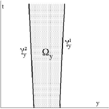
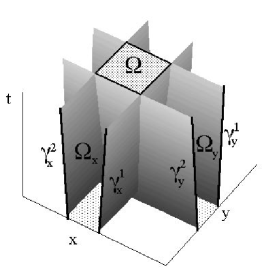
Figure 4: The emission coordinates $\tau_{x}^{1},\tau_{x}^{2}$ are defined in the coordinate domain $\Omega_{x}$, which is the space-time region between the two emitters world-lines; the same holds for the emission coordinates $\tau_{y}^{1},\tau_{y}^{2}$ defined in $\Omega_{y}$. Then, the set of emission coordinates $\tau_{x}^{1},\tau_{x}^{2},\tau_{y}^{1},\tau_{y}^{2}$ is well defined in $\Omega=\Omega_{x}\cap\Omega_{y}$

After having described some examples of the definition of emission coordinates in 1+1 dimensional space-times, now we aim at exploiting the framework outlined so far in order to set up a system of emission coordinates capable of mapping a more realistic 1+3 dimensional space-time, thanks to a suitable set of emitters. Actually, these emitters will be chosen in order to allow an easy manage of the map between Cartesian and emission coordinates: in other words, we will consider some toy models that, nonetheless, enable us to show the underlying ideas of the emission coordinates approach to positioning systems.

We start, in next Section, by considering the case of a flat four dimensional space-time. Then, in the subsequent Section, we introduce a small inhomogenity, i.e. a small gravitational field, and discuss some possible applications.

VI.1 Flat space-time case

Let us consider three pairs of satellites, provided with clocks and emitters, each of them moving, with constant speed, along a coordinate axis in a flat Minkwoski background. The particular choice of the satellites allows to benefit from what we have done in the 2-dimensional case above. In fact, for each pair of satellites, the metric

$$ds^{2}=dt^{2}-dx^{2}-dy^{2}-dz^{2},$$ (55)

reduces to

$$ds^{2}=dt^{2}-(dx^{i})^{2}\quad\quad i=1,2,3.$$ (56)

In particular, the metric (56) allows to easily introduce null coordinates $u,v$ as we have done in Section III: this can be done for each pair of satellites.

To be precise, recalling the notation introduced in Section III, we can label the world-lines of each pair of satellites as follows

$$\gamma_{a}^{1}\equiv\begin{cases}\,{u}_{a}=\lambda_{a}^{1}\tau_{a}^{1}\\[2.84526pt] \,{v}_{a}=\displaystyle\frac{1}{\lambda_{a}^{1}}\tau_{a}^{1}+v_{a0}\end{cases}\ \gamma_{a}^{2}\equiv\begin{cases}\,{u}_{a}=\lambda_{a}^{2}\tau_{a}^{2}+u_{a0}\\[2.84526pt] \,{v}_{a}=\displaystyle\frac{1}{\lambda_{a}^{2}}\tau_{a}^{2}\end{cases}\quad\quad a=x,y,z.$$ (57)

Then, if we consider the pair of satellites moving along the $x$ axis, eq. (21) tells us that the relations between the cartesian coordinates $\tilde{t},\tilde{x}$ and emission coordinates $\tau^{1},\tau^{2}$ of the point $P$ are:

$$\tilde{t}=\frac{1}{2}\left(\lambda^{1}_{x}\tau_{x}^{1}+\frac{\tau_{x}^{2}}{\lambda_{x}^{2}}\right)\quad\quad\tilde{x}=\frac{1}{2}\left(\lambda_{x}^{1}\tau_{x}^{1}-\frac{\tau_{x}^{2}}{\lambda_{x}^{2}}\right).$$ (58)

The same procedure that we have just outlined can be repeated considering the other two pairs of satellites moving along the $y$ and $z$ axes. In doing so, we obtain the following expressions for the coordinates $\tilde{t},\tilde{y},\tilde{z}$ of the point $P$, in terms of the proper times $\tau_{y}^{1},\tau_{y}^{2},\tau_{z}^{1},\tau_{z}^{2}$:

$$\tilde{t}=\frac{1}{2}\left(\lambda^{1}_{y}\tau_{y}^{1}+\frac{\tau_{y}^{2}}{\lambda_{y}^{2}}\right)\quad\quad\tilde{y}=\frac{1}{2}\left(\lambda_{y}^{1}\tau_{y}^{1}-\frac{\tau_{y}^{2}}{\lambda_{y}^{2}}\right),$$ (59)

$$\tilde{t}=\frac{1}{2}\left(\lambda^{1}_{z}\tau_{z}^{1}+\frac{\tau_{z}^{2}}{\lambda_{z}^{2}}\right)\quad\quad\tilde{z}=\frac{1}{2}\left(\lambda_{z}^{1}\tau_{z}^{1}-\frac{\tau_{z}^{2}}{\lambda_{z}^{2}}\right).$$ (60)

Summarizing, this procedure allows us to write the cartesian coordinates $\tilde{t},\tilde{x},\tilde{y},\tilde{z}$ of the point $P$ in terms of the 6 proper times $\tau_{x}^{1},\tau_{x}^{2},\tau_{y}^{1},\tau_{y}^{2},\tau_{z}^{1},\tau_{z}^{2}$. Of course, the expressions (58-60) are redundant, since the coordinate $\tilde{t}$ is the same for all. This fact can be exploited in order to eliminate 2 of the 6 proper times, which means that 4 satellites would be enough, as can be expected from the dimensions of space-time. For instance, we may use the constraints

$$\tilde{t}(\tau_{x}^{1},\tau_{x}^{2})=\tilde{t}(\tau_{y}^{1},\tau_{y}^{2}),$$ (61)

and

$$\tilde{t}(\tau_{x}^{1},\tau_{x}^{2})=\tilde{t}(\tau_{z}^{1},\tau_{z}^{2}),$$ (62)

to express $\tau_{2}^{y}$ as a function of $\tau_{x}^{1},\tau_{x}^{2},\tau_{y}^{1}$ and $\tau_{2}^{z}$ as a function of $\tau_{x}^{1},\tau_{x}^{2},\tau_{z}^{1}$, respectively. Consequently, eqs. (58-60) and (61), (62) allows us to express the cartesian coordinates $\tilde{t},\tilde{x},\tilde{y},\tilde{z}$ of the point $P$ in terms of the 4 proper times $\tau_{x}^{1},\tau_{x}^{2},\tau_{y}^{1},\tau_{z}^{1}$:

$$\tilde{t} = \tilde{t}\left(\tau_{x}^{1},\tau_{x}^{2},\tau_{y}^{1},\tau_{z}^{1}\right)$$ (63)

$$\tilde{x} = \tilde{x}\left(\tau_{x}^{1},\tau_{x}^{2},\tau_{y}^{1},\tau_{z}^{1}\right)$$ (64)

$$\tilde{y} = \tilde{y}\left(\tau_{x}^{1},\tau_{x}^{2},\tau_{y}^{1},\tau_{z}^{1}\right)$$ (65)

$$\tilde{z} = \tilde{z}\left(\tau_{x}^{1},\tau_{x}^{2},\tau_{y}^{1},\tau_{z}^{1}\right).$$ (66)

Remark. According to our approach, each pair of emission coordinates $\tau_{a}^{1},\tau_{a}^{2}$ is well defined in the corresponding coordinate domain $\Omega_{a}$ (see Section II and figure 1) which, in turn, depends on the emitters world-lines. So, if we use more pairs of emission coordinates, the full coordinate domain $\Omega$ is the intersection of the coordinate domains $\Omega_{a}$. For instance, if we consider in the 1+2 dimensional space-time the emission coordinates $\tau_{x}^{1},\tau_{x}^{2}$ defined in $\Omega_{x}$, and $\tau_{y}^{1},\tau_{y}^{2}$ defined in $\Omega_{y}$, the set of emission coordinates $\tau_{x}^{1},\tau_{x}^{2},\tau_{y}^{1},\tau_{y}^{2}$ is well defined in $\Omega=\Omega_{x}\cap\Omega_{y}$ (see figure 4). This obviously can be generalized to the 1+3 dimensional space-time.

If we explicitly write the equations (63-66), we see that the relation between the Cartesian and emission coordinates is given by the following linear map:

$$\bm{X}=\bm{A}\cdot\bm{T},$$ (67)

where

$$\bm{X}\doteq\left(\begin{array}[]{c}\tilde{t}\\ \tilde{x}\\ \tilde{y}\\ \tilde{z}\\ \end{array}\right),$$ (68)

$$\bm{T}\doteq\left(\begin{array}[]{c}\tau_{x}^{1}\\ \tau_{x}^{2}\\ \tau_{y}^{1}\\ \tau_{z}^{1}\\ \end{array}\right),$$ (69)

and the coordinate change matrix $\bm{A}$ is defined by

$$\bm{A}\doteq\left(\begin{array}[]{cccc}\frac{\lambda_{x}^{1}}{2}&\frac{1}{2\lambda_{x}^{2}}&0&0\\ \frac{\lambda_{x}^{1}}{2}&\frac{1}{2\lambda_{x}^{2}}&0&0\\ -\frac{\lambda_{x}^{1}}{2}&-\frac{1}{2\lambda_{x}^{2}}&\lambda_{y}^{1}&0\\ -\frac{\lambda_{x}^{1}}{2}&-\frac{1}{2\lambda_{x}^{2}}&0&\lambda_{z}^{1}.\\ &&&\end{array}\right)$$ (70)

It is easy to show that $det(\bm{A})=-\frac{\lambda_{x}^{1}\lambda_{y}^{1}\lambda_{z}^{1}}{2\lambda_{x}^{2}}$ so that it is generally different from zero.

The inverse metric is given by

$$\bm{A}^{-1}\doteq\left(\begin{array}[]{cccc}\frac{1}{\lambda^{1}_{x}}&\frac{1}{\lambda^{1}_{x}}&0&0\\ \lambda^{2}_{x}&-\lambda^{2}_{x}&0&0\\ \frac{1}{\lambda^{1}_{y}}&0&\frac{1}{\lambda^{1}_{y}}&0\\ \frac{1}{\lambda^{1}_{z}}&0&0&\frac{1}{\lambda^{1}_{z}}.\\ &&&\end{array}\right)$$ (71)

Actually, the choice of the emission coordinates is somewhat arbitrary: in other words, in the approach we have just outlined, we can choose 12 sets of emission coordinates. In fact, we must receive signals from satellites propagating along all axes, in order to have a map of the whole space; this implies that 2 signals must come from satellites propagating along the same direction, and the other two signals must come from satellites propagating along the remaining directions. The latter can be arranged according to 4 combination: for instance, if we choose that two signals come from satellites propagating along the $x$ directions, the corresponding combinations of emission coordinates are:

$$\begin{array}[]{cccc}\tau_{x}^{1}&\tau_{x}^{2}&\tau_{y}^{1}&\tau_{z}^{1}\\ \tau_{x}^{1}&\tau_{x}^{2}&\tau_{y}^{1}&\tau_{z}^{2}\\ \tau_{x}^{1}&\tau_{x}^{2}&\tau_{y}^{2}&\tau_{z}^{1}\\ \tau_{x}^{1}&\tau_{x}^{2}&\tau_{y}^{2}&\tau_{z}^{2}\\ &&&\end{array}$$ (72)

The same argument applies if we choose that two signals come from satellites propagating along the $y$ and $z$ directions, so that, summarizing, we have 12 possible choices of coordinates. We point out that the coordinate domain $\Omega$ is the intersection of the coordinate domain $\Omega_{a}$ (see the previous Remark). Finally, we notice that, in this approach, the uncertainties on the Cartesian coordinates can be expressed in terms of the uncertainties on the emission coordinates and on the parameters of the world-lines.

VI.2 Quasi-flat space-time case

Let us consider the space-time described by the metric:

$$ds^{2}=(1+gx^{2})dt^{2}-dx^{2}-dy^{2}-dz^{2}.$$ (73)

In the space-time described by (73), we consider three pairs of emitters as follows: two pairs are moving along the $y$ and $z$ axis, with constant speed, so that the metric (73) reduces to

$$ds^{2}=dt^{2}-(dx^{i})^{2}\quad\quad i=2,3.$$ (74)

The other two emitters, are at rest, at $x=x^{1},x=x^{2}$, where $x^{1},x^{2}$ are constant, in the $x,t$ plane (their $y,z$ coordinates are null). For them, the metric (73) reduces to

$$ds^{2}=(1+gx)^{2}dt^{2}.$$ (75)

In particular, we may apply the formalism of section III to the first two pairs of satellites, and the formalism of section V to the last pair of satellites.

On doing so, we want to express the coordinate $\tilde{t},\tilde{x},\tilde{y},\tilde{z}$ of a point $P$ in terms of emission coordinates, as we have done in Section VI.1 above.

Recalling the results of section V (from which we borrow hypotheses and notation), we know that we may write

$$\tilde{t}=\left(1-g\tilde{x}\right)\frac{\tau^{1}_{x}-\tau^{1}_{x0}+\tau^{2}_{x}-\tau^{2}_{x0}+x^{1}-x^{2}}{2}\quad\tilde{x}=\frac{\tau^{1}_{x}-\tau^{1}_{x0}-\left(\tau^{2}_{x}-\tau^{2}_{x0}\right)+x^{1}+x^{2}}{2},$$ (76)

and

$$\tilde{t}=\frac{1}{2}\left(\lambda^{1}_{y}\tau_{y}^{1}+\frac{\tau_{y}^{2}}{\lambda_{y}^{2}}\right)\quad\quad\tilde{y}=\frac{1}{2}\left(\lambda_{y}^{1}\tau_{y}^{1}-\frac{\tau_{y}^{2}}{\lambda_{y}^{2}}\right),$$ (77)

$$\tilde{t}=\frac{1}{2}\left(\lambda^{1}_{z}\tau_{z}^{1}+\frac{\tau_{z}^{2}}{\lambda_{z}^{2}}\right)\quad\quad\tilde{z}=\frac{1}{2}\left(\lambda_{z}^{1}\tau_{z}^{1}-\frac{\tau_{z}^{2}}{\lambda_{z}^{2}}\right).$$ (78)

As a consequence, the Cartesian coordinates $\tilde{t},\tilde{x},\tilde{y},\tilde{z}$ of the point $P$ are known in terms of the 6 proper times $\tau_{x}^{1},\tau_{x}^{2},\tau_{y}^{1},\tau_{y}^{2},\tau_{z}^{1},\tau_{z}^{2}$. Again, the expressions (76-78) are redundant, since the coordinate $\tilde{t}$ is the same for all. This fact can be exploited in order to eliminate 2 of the 6 proper times. If we use the constraints

$$\tilde{t}(\tau_{x}^{1},\tau_{x}^{2})=\tilde{t}(\tau_{y}^{1},\tau_{y}^{2}),$$ (79)

and

$$\tilde{t}(\tau_{x}^{1},\tau_{x}^{2})=\tilde{t}(\tau_{z}^{1},\tau_{z}^{2}),$$ (80)

we may express $\tau_{2}^{y}$ as a function of $\tau_{x}^{1},\tau_{x}^{2},\tau_{y}^{1}$ and $\tau_{2}^{z}$ as a function of $\tau_{x}^{1},\tau_{x}^{2},\tau_{z}^{1}$, respectively. Consequently, eqs. (76-78) and (79-80) allow us to express the Cartesian coordinates $\tilde{t},\tilde{x},\tilde{y},\tilde{z}$ of the point $P$ in terms of the 4 proper times $\tau_{x}^{1},\tau_{x}^{2},\tau_{y}^{1},\tau_{z}^{1}$. Also in this case, the coordinate domain $\Omega$ is determined by the intersection of the coordinate domains $\Omega_{a}$ where each pair of emission coordinates $\tau_{a}^{1},\tau_{a}^{2}$ is defined (see the Remark in Section VI.1),

An important difference with the purely flat case described in Section VI.1 is that now a non linear relation between the Cartesian and emission coordinates arises, due to the presence of the acceleration $g$. However, we may write the explicit relations:

$$\tilde{t} = a\tau^{1}_{x}+b(\tau^{1}_{x})^{2}+c\tau^{2}_{x}+d(\tau^{2}_{x})^{2}+e+f+g$$ (81)

$$\tilde{x} = \frac{\tau^{1}_{x}-\tau^{1}_{x0}}{2}-\frac{\tau^{2}_{x}-\tau^{2}_{x0}}{2}+\frac{x^{1}+x^{2}}{2}$$ (82)

$$\tilde{y} = -a\tau^{1}_{x}-b(\tau^{1}_{x})^{2}-c\tau^{2}_{x}-d(\tau^{2}_{x})^{2}-e-f-g+\lambda^{1}_{y}\tau^{1}_{y}$$ (83)

$$\tilde{z} = -a\tau^{1}_{x}-b(\tau^{1}_{x})^{2}-c\tau^{2}_{x}-d(\tau^{2}_{x})^{2}-e-f-g+\lambda^{1}_{z}\tau^{1}_{z}$$ (84)

where

$$a = \frac{1}{2}g\tau^{1}_{x0}-\frac{1}{2}gx^{1}+\frac{1}{2}$$ (85)

$$b = -\frac{g}{4}$$ (86)

$$c = -\frac{1}{2}g\tau^{2}_{x0}-\frac{1}{2}gx^{2}+\frac{1}{2}$$ (87)

$$d = \frac{g}{4}$$ (88)

$$e = \frac{g}{4}\left((x^{2})^{2}-(x^{1})^{2}+(\tau^{2}_{x0})^{2}-(\tau^{1}_{x0})+2\tau^{1}_{x0}x^{1}+2\tau^{2}_{x0}x^{2}\right)$$ (89)

$$f = \frac{x^{1}-x^{2}}{2}$$ (90)

$$g = -\frac{\tau^{1}_{x0}+\tau^{2}_{x0}}{2}$$ (91)

VII Conclusions

In this work we have built explicit maps from Cartesian coordinates to emission coordinates, for suitably chosen set of emitters, starting from the underlying assumption of knowing the whole details of the emitters world-lines, i.e., for instance the velocities and the positions at a given time. The approach that we have outlined allows us to express the uncertainties on the Cartesian coordinates in terms of the uncertainties on the emission coordinates and on the parameters of the world-lines; the definition of the coordinate domain (i.e. the space-time region where the emission coordinates are unambiguously defined) depends on the emitters world-lines.

In particular, we have obtained explicit maps in Minkowski 1+1 dimensional space-time, for inertial emitters and accelerated ones. The latter can be also interpreted as emitters at rest in a gravitational field. The same procedure has been generalized to 1+3 dimensional space time, both in the inertial case and in the case where a small ”gravitational” field has been introduced. Actually, in order to give a more operational definition of the emission coordinates systems more general and realistic situations should be studied, nonetheless the toy models that we have studied here are suitable to suggest the basic ideas of this fully relativistic approach to positioning systems.

References

• (1) Ashby N., in Relativity in Rotating Frames, eds. Rizzi G. and Ruggiero M.L., in the series “Fundamental Theories of Physics”, Kluwer Academic Publishers, Dordrecht (2004)
• (2) Ashby N., in Living Rev. Relativity 6, http://www.livingreviews.org/lrr-2003-1 (2003)
• (3) Coll B., in Proceedings of 28th Spanish Relativity Meeting (ERE05), published in AIP Conf.Proc. 841, 277 (2006), gr-qc/0601110
• (4) Coll B., Pozo J.M., Class. Quant. Grav. 23, 7395 (2006), gr-qc/0606044
• (5) Ferrando J.J., Proceedings of 28th Spanish Relativity Meeting (ERE05), published in AIP Conf.Proc. 841, 424 (2006), gr-qc/0601117
• (6) Coll B., Ferrando J.J., Morales J.A., Phys. Rev. D 73, 084017 (2006), gr-qc/0602015
• (7) Coll B., Ferrando J.J., Morales J.A., Phys. Rev. D 74, 104003 (2006), gr-qc/0607037
• (8) Møller C., The Theory of Relativity, Oxford University Press, Oxford (1972)