Primordial magnetic fields at preheating.

Abstract:

Using lattice techniques we investigate the generation of long range cosmological magnetic fields during a cold electroweak transition. We will show how magnetic fields arise, during bubble collisions, in the form of magnetic strings. We conjecture that these magnetic strings originate from the alignment of magnetic dipoles associated with EW sphaleron-like configurations. We also discuss the early thermalisation of photons and the turbulent behaviour of the scalar fields after tachyonic preheating.

1 Introduction.

There have been many theoretical attempts to explain the origin of large scale cosmological magnetic fields (LSMF) [1]. The main difficulty resides in understanding their correlation scale which ranges from the size of galaxies to clusters and super-clusters with an amplitude of the order of micro-gauss, pointing to a primordial origin. Following the work initiated in [2], we address this issue in the context of a cold electroweak transition taking place after a period of hybrid inflation. The EW transition has been in the heart of many proposals to address magnetogenesis, linking it in many cases with the generation of the baryon asymmetry. The results presented here resemble the mechanism proposed by Vachaspati connecting the appearance of magnetic fields to that of sphalerons and Z-strings [3].

The model we have considered is a hybrid inflation model with the bosonic field content of the Standard Model coupled, via the Higgs field, to a singlet inflaton:

$${\cal L}=-\frac{1}{4}G^{a}_{\mu\nu}G^{\mu\nu}_{a}-\frac{1}{4}F^{Y}_{\mu\nu}F_{Y}^{\mu\nu}+{\rm Tr}\Big{[}(D_{\mu}\Phi)^{\dagger}D^{\mu}\Phi\Big{]}+\frac{1}{2}(\partial_{\mu}\chi)^{2}-V(\Phi,\chi)$$ (1)

$${\rm V}(\Phi,\chi)={\rm V}_{0}+\frac{1}{2}(g^{2}\chi^{2}-m^{2})\,|\Phi|^{2}+\frac{\lambda}{4}|\Phi|^{4}+\frac{1}{2}\mu^{2}\chi^{2}\,$$ (2)

The couplings are fixed to the standard model values for several ratios of the Higgs to W masses. For concreteness, we have fixed the inflaton to Higgs coupling by the relation: $g^{2}=2\lambda$. To solve the time evolution of the system, starting at the end of inflation, we have performed a numerical evolution based on a suitable classical approximation (more details can be found in Refs. [4, 2, 5]). In this work we discuss the results for $M_{\rm H}=4.65\ M_{\rm W}$. Results for more realistic values will be presented in [5].

2 Simulation results.

The evolution of the scalars shows two regimes that determine the behaviour of the system. The first one is the spontaneous symmetry breaking (SSB) stage which proceeds via the generation, expansion and collision of bubble-like structures in the Higgs field [4]. It is in this regime where a rich phenomenology can arise, including the generation of the baryon asymmetry of the Universe and a stochastic background of gravitational waves, see Refs. [4, 6, 7, 8], and where we place the origin of the LSMF. In our simulations this regime starts right after the end of inflation ($mt\!\sim\!5\!-\!10$ for $M_{\rm H}=4.65\ M_{\rm W}$) and lasts until times of order $mt\!\sim\!35\!-\!40$. After this relatively short stage, a period of slow approach to equilibrium follows where two important phenomena appear: turbulence and thermalisation of high momentum photons.

2.1 First regime: Generation of magnetic fields.

The simulations show that magnetic fields are predominantly generated in the SSB regime. We have already mentioned that bubble collisions are responsible for SSB. Bubbles originate at peaks of the initial Higgs Gaussian random field and expand from there on [4]. As exhibited in Fig. 1 (Left), the regions between bubbles remain for a longer time in the false vacuum, giving rise to string-like structures of local minima of the Higgs-field. Strongly correlated with them, magnetic fields appear dominantly in the form of magnetic strings, see Fig. 1 (Right). We conjecture that these magnetic strings originate from sphaleron-like configurations which are copiously produced during SSB at the location of Higgs-field zeroes [4, 8]. For non-zero Weinberg angle the magnetic field generated by the sphaleron looks like a magnetic dipole [11, 12]. Then, as in a ferromagnetic material, these dipoles would tend to align along the string of Higgs-zeroes generating a magnetic string. One remark has to be done concerning Fig. 1. The plot has a lower cutoff giving the impression that magnetic lines are open. This is just a projection effect, and places where the magnetic strings seem to end are just places where the magnetic flux spreads.

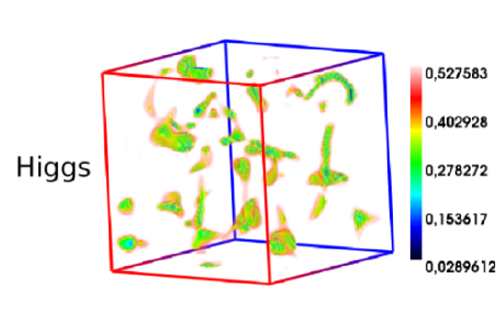
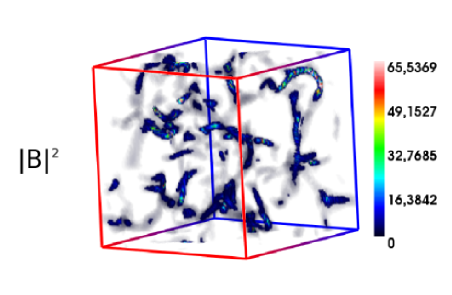
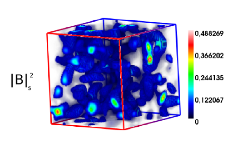
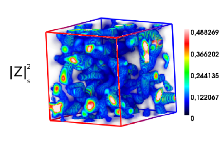
Figure 1: Top: (Left) Locus of points where the value of the Higgs norm is below $0.53$. (Right) Locus of points where the U(1)-magnetic energy is above $1.5$. Bottom: (Left) Smeared density of the U(1)-magnetic energy. (Right) Smeared density of the magnetic component of the Z field. Both above 0.1. All at $mt=15$.

The picture that we extract resembles the mechanism proposed in Ref. [3], in which magnetic strings also appear at the electroweak phase transition, and are related to Z-strings. The bottom half of Fig. 1 shows the smeared Z-magnetic field together with the smeared U(1)-magnetic field at $mt=~{}15$. The correlation is manifest. In this plot the string structure has been enhanced by performing smearing (averaging the fields over the neighborhood of a point). This helps in two ways: first, it smooths the central singularities of the strings and secondly, it clears up the radiation background of non-coherent fields. The procedure respects the regions where the scales are roughly constant and does not disturb the whole picture as far as the neighborhood involved in the averaging is smaller than the width of the string ($\sim 1/M_{\rm W}$).

Having a mechanism for generating magnetic fields, two important questions arise, and the viability of this mechanism as LSMF generator depends on their answer. These questions are:

• Are the scales of the generated magnetic fields large enough to be the seed of LSMF?

• Do they persist in time long enough to be used as seeds of LSMF?

A qualitative answer to the first question can be extracted from Fig. 1. Individual strings merge due to magnetic reconnection forming a cluster of the order of the box size. This merging of individual strings is essential to enhance the large scale structure of the fields. In order to give a quantitative measure of the nature of the magnetic field objects as actual strings, we have analysed the following quantity:

$$B_{L}(r_{0})=\frac{1}{L^{3}}\int_{L(r_{0})}dx^{3}B^{2}(x)\,,$$ (3)

where the integration is on a box of length $L$, centered at a point $r_{0}$ belonging to one of the strings. Figure 2 (Left) shows the $L$ dependence of $L^{2}B_{L}(r_{0})$, averaged over several configurations. The expected behaviour of $B_{L}(r_{0})$ if $r_{0}$ is in the central core of a string-like object is clear. Inside the string the magnetic intensity is roughly constant, so the integral goes like the volume of the box and $B_{L}(r_{0})$ is constant. Once the size of the box gets larger than the diameter of the string, the integral only grows along the direction of the string and $B_{L}(r_{0})\sim L^{-2}$. This gives the plateau seen in the figure. The small errors indicate that the string objects are quite configuration independent.The length of the plateau provides an estimate of the minimal length of the string as an isolated object. It indicates a mean minimal string length of order $M_{\rm W}L\sim 4-5$, which is a significant part of the total length. For larger values of $L$ the merging of strings and the fact that more strings are entering the box, change the behaviour to a volume like one, with $B_{L}(r_{0})$ roughly constant.

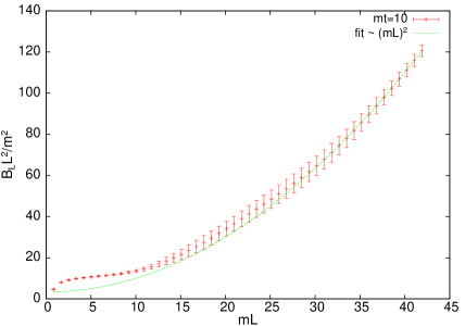
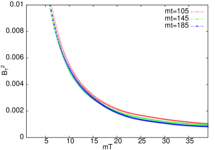
Figure 2: Left: Averaged $B_{L}(r_{0})$, Eq. (2.1), at $mt=10$. The center of the box is chosen to be the maximum value in the center of a string. The plateau length provides an estimate of the minimal length of a representative string. Right: Dependence of $B_{T}^{2}\equiv\langle\vec{B}_{T}^{2}\rangle$ on the time-interval length $T$, see Eq. (2.2). $B_{T}^{2}$ is normalized to the total energy density.

The time persistence analysis is quite more subtle. A detailed analysis of the behaviour in time of the low momentum magnetic field spectra is on the way and will be presented in [5]. Some preliminary conclusions can already be presented here. A time average can be defined as follows:

$$\vec{B}_{T}(t_{0})=\frac{1}{T}\int_{T(t_{0})}dt\vec{B}(t),$$ (4)

this is, the integral over a time interval of length $T$ that starts at $t_{0}$. This time-averaging can be seen as a way to eliminate short scale magnetic fields, as the radiation fields. For instance, for a monochromatic wave,

$$\langle|\vec{B}_{T}|^{2}\rangle\sim\frac{1}{V}\int dk|\vec{B}_{k}|^{2}\ W^{2}(k,T)\;,\;W=\frac{sin(|k|T/2)}{|k|T/2},$$ (5)

where the average is both over space and configurations. For large $T$, momenta with $|k|>>(T)^{-1}$ are suppressed. We can use that to estimate the length of the time interval for which all momenta but our minimal momenta $p_{\rm min}=2\pi/L$ are suppressed. This gives a window of possible intensities of the magnetic seeds coherent at scales larger or equal to the scale given by the size of the box. Fig. 2 (Right) shows the dependence of $\langle|\vec{B}_{T}|^{2}\rangle$, normalized to the total energy density ($\rho_{0}$), on the length of the time interval $T$, for $p_{\rm min}=0.15m$. Note that the average turns out to be quite independent of the starting point of the averaging $t_{0}$, indicating that the sub-leading large scales are quite independent of time. From the values above $mT\sim 6$ we obtain a window $\langle\vec{B}_{T}^{2}\rangle\sim[10^{-2},10^{-3}]\ \rho_{0}$. Assuming the magnetic field expands as radiation, this would give magnetic fields today of order $[1,0.3]\mu G$, which are in the range of the observed ones in galaxies, and even in clusters of galaxies, where no-extra amplification through a dynamo mechanisms is expected.

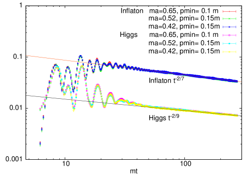
Figure 3: Scalar variances, Eq. (2.4), plotted in logarithmic scale for different lattice spacings and volumes.

2.2 Second regime: Turbulence and photon thermalisation.

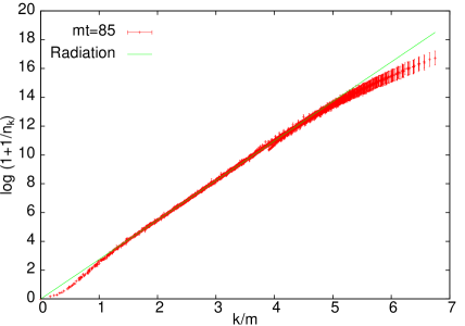
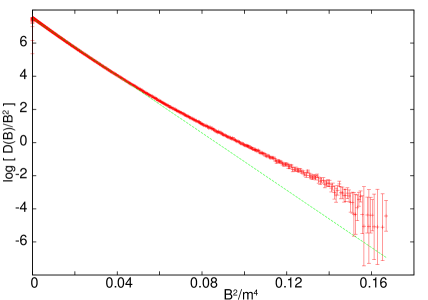
Figure 4: Left: $\rm{log}(n_{k}^{-1}+1)$ and Right: $\rm{log}(D(B)/B^{2})$, Eq. (2.5), for the spectrum of photon radiation at times $mt=85$ and $mt=225$ respectively.

Once the SSB takes place, the system starts a slow approach to equilibrium. This proceeds via a period in which the scalars and also some of the gauge degrees of freedom undergo a turbulent regime. Turbulence in the scalar fields manifests through the time evolution of their variances shown in Fig. 3. As predicted by [10] and also shown in [2, 9], variances follow the law:

$$\langle f^{2}\rangle-\langle f\rangle^{2}\sim t^{-\nu}\,;\hskip 14.22636pt\nu={2\over(2m-1)},$$ (6)

for $m$-particle interactions and $f$ denoting each of the scalars. The change in model parameters with respect to [2], where $M_{\rm W}=6$ GeV, results in a modification of the turbulent behaviour. The parameter $m$, now turns out to be $m=5(4)$ for the Higgs (inflaton), which differs from the former $m=4(3)$ obtained in [2], but is in agreement with [9].

In Ref. [2] we showed the self-similarity of the momentum spectra of the SU(2) degrees of freedom long after SSB. This additional sign of turbulence indicated a departure from thermal equilibrium. High momentum photons, however, thermalise very early in the evolution. In thermal equilibrium the radiation occupation number is expected to behave according to the Bose-Einstein distribution: $n_{k}=(\exp(\beta k)-1)^{-1}$, from where the thermalisation temperature can be extracted. Fig. 4 (Left) represents $\ln(1+n_{k}^{-1})$ for photon radiation. Photons with momenta above $m$ follow the Bose-Einstein law. The temperature extracted is of the order of $M_{\rm W}$ from times $mt\sim 40$ on. Thermalisation is corroborated by analysing the distribution of norms of the magnetic field. In thermal equilibrium this distribution is given by [5]:

$$D(B)=B^{2}\ e^{-3B^{2}/(2\langle B^{2}\rangle)}\,;\hskip 14.22636pt\langle B^{2}\rangle=\frac{\pi^{2}T^{4}}{15}$$ (7)

Fig. 4 right shows $D(B)$. From time $mt\sim 40$ on the equilibrium distribution is reached, with a temperature in agreement with the one extracted from the spectra. In both plots a systematic deviation from the thermal behaviour is observed at the low momenta, large norm, part of the fits. It is there where the interesting magnetic string structures reside. An analysis of the possible, late time, turbulent and helical behaviour of the low momentum part of the magnetic field spectrum is on the way and will be reported elsewhere.

3 Conclusions.

We have analysed numerically the proposal that long range magnetic fields could be generated during a cold electroweak transition after a period of low scale hybrid inflation. The generation mechanism is mainly based on two facts:

• At the SSB stage bubble-like structures, associated to local maxima in the Higgs-field norm, appear. Points outside the bubble front, remaining close to the false vacuum, form string like structures.

• Bubble collisions give rise to sphaleron-like configurations attached to the location of zeroes of the Higgs field. For $\theta_{W}\neq 0$ these sphalerons behave as magnetic dipoles.

These two ingredients together lead to an allignment of the sphalerons’ dipoles forming magnetic string networks as we have observed in our simulations. Some results concerning the coherence and intensity of the generated magnetic fields have been presented. A further analysis of the time evolution of the magnetic field, as well as the study of the dependence of the $M_{\rm H}$ to $M_{\rm W}$ ratio will be presented in [5].

We have also discussed some features of the late time behaviour of the system, among them, thermalisation of photon radiation and turbulence in the scalar fields.

- [1] M. Giovanini, Int. J. Mod. Phys. D 13 (2004) 391; D. Grasso and H.R. Rubinstein, Phys. Rept. 348, 163 (2001).
- [2] A. Díaz-Gil, J. García-Bellido, M. García Pérez, A. González-Arroyo, in proceedings of Lattice 2005 conference, \posPoS(LAT2005) 242.
- [3] T. Vachaspati, Phys. Lett. B 265, 258 (1991); Phys. Rev. Lett. 87, 251302 (2001).
- [4] J. García-Bellido, M. García Pérez and A. González-Arroyo, Phys. Rev. D 67 (2003) 103501; Phys. Rev. D 69 (2004) 023504.
- [5] A. Díaz-Gil, J. García-Bellido, M. García Pérez, A. González-Arroyo, in preparation.
- [6] J. García-Bellido, D. Y. Grigoriev, A. Kusenko and M. E. Shaposhnikov, Phys. Rev. D 60 (1999) 123504; L. M. Krauss and M. Trodden, Phys. Rev. Lett. 83 (1999) 1502.
- [7] J. Smit, in proceedings of Lattice 2005 conference, \posPoS(LAT2005) 022, and references therein.
- [8] J.Smit, A.Tranberg, JHEP 12 (2002) 020; JHEP 0311 (2003) 016; JHEP 0608 (2006) 012; J. I. Skullerud, J. Smit and A. Tranberg, JHEP 0308 (2003) 045; M. van der Meulen, D. Sexty, J. Smit and A. Tranberg, JHEP 0602 (2006) 029; A. Tranberg, J. Smit and M. Hindmarsh, JHEP 0701 (2007) 034.
- [9] J. García-Bellido, D. G. Figueroa, Phys. Rev. Lett. 98 (2007) 061302; J. García-Bellido, D. G. Figueroa and A. Sastre, e-Print: arXiv:0707.0839 [hep-ph] (2007)
- [10] R. Micha and I. I. Tkachev, Phys. Rev. D 70 (2004) 043538; Phys. Rev. Lett. 90 (2003) 121301.
- [11] F. Klinkhamer and N. Manton, Phys. Rev. D 30 (1984) 2212; J. Kunz, B. Kleihaus and Y. Brihaye, Phys. Rev. D 46 (1992) 3587; Phys. Lett. B 273 (1991) 100.
- [12] M. Hindmarsh and M. James, Phys.Rev. D 49 (1994) 6109.