Late stages of the evolution of A-type stars on the main sequence: comparison between observed chemical abundances and diffusion models for 8 Am stars of the Praesepe cluster

Abstract

Aims. We aim to provide observational constraints on diffusion models that predict peculiar chemical abundances in the atmospheres of Am stars. We also intend to check if chemical peculiarities and slow rotation can be explained by the presence of a weak magnetic field.

Methods. We have obtained high resolution, high signal-to-noise ratio spectra of eight previously-classified Am stars, two normal A-type stars and one Blue Straggler, considered to be members of the Praesepe cluster. For all of these stars we have determined fundamental parameters and photospheric abundances for a large number of chemical elements, with a higher precision than was ever obtained before for this cluster. For seven of these stars we also obtained spectra in circular polarization and applied the LSD technique to constrain the longitudinal magnetic field.

Results. No magnetic field was detected in any of the analysed stars. HD 73666, a Blue Straggler previously considered as an Ap (Si) star, turns out to have the abundances of a normal A-type star. Am classification is not confirmed for HD 72942. For HD 73709 we have also calculated synthetic $\Delta a$ photometry that is in good agreement with the observations. There is a generally good agreement between abundance predictions of diffusion models and values that we have obtained for the remaining Am stars. However, the observed Na and S abundances deviate from the predictions by 0.6 dex and $\geq$0.25 dex respectively. Li appears to be overabundant in three stars of our sample.

1 Introduction

Main sequence A-type stars present spectral peculiarities, usually interpreted as due to peculiar photospheric abundances and abundance distributions which are believed to be produced by the interaction of a large variety of physical processes (e.g. diffusion, magnetic field, pulsation and various kinds of mixing processes).

An interesting problem that has yet to be addressed is how these peculiarities change during main sequence evolution. The chemical composition of field A-type stars have been studied by several authors, e.g. Hill & Landstreet (1993), Adelman et al. (2000). However, it is not straightforward to use the results of these investigations to study how photospheric chemistry evolves during a star’s main sequence life. First, the original composition of the cloud from which stars were born is not known and is likely somewhat different for each field star. It is therefore not possible to discriminate between evolutionary effects and differences due to original chemical composition. Secondly, it is difficult to estimate the age of field stars with the precision necessary for such evolutionary studies (for a discussion of this problem see Bagnulo et al. 2006).

From this point of view, A-type stars belonging to open clusters are much more interesting objects. Compared to field stars, A-type stars in open clusters have three very interesting properties:

• they were all presumably born from the interstellar gas with an approximately uniform composition;

• they all have approximately the same age (to within a few Myr);

• their age can be determined much more precisely than for field stars.

Few abundance analyses of A-type stars in open clusters have been carried out. Those that have been published have usually focused on a limited numbers of stars.

Varenne & Monier (1999) have determined the abundances of eleven chemical elements for a large sample of stars regularly distributed in spectral type along the main sequence in order to sample the expected masses uniformly. All these stars were analysed in a uniform manner using spectrum synthesis. Stütz et al. (2006) have performed a detailed abundance analysis for five A-type stars of the young open cluster IC 2391. Folsom et al. (2007) have performed a detailed abundance analysis for four Ap/Bp stars and one normal late B-type star of the open cluster NGC 6475.

A goal of this programme is to determine photospheric abundance patterns in A-type star members of clusters of different ages. This is crucial in order to: i) investigate the chemical differences between normal and peculiar stars inside the same cluster, ii) study the evolution with time of abundance peculiarities by studying clusters of various ages, iii) set constraints on the hydrodynamical processes occurring at the base of the convection zone in the non magnetic stars and iv) study the effects of diffusion in the presence of a magnetic field for the magnetic (Ap) stars in the cluster. The abundance analysis will be performed in an homogeneous way applying a method described in this first work.

Praesepe (NGC 2632), a nearby intermediate-age open cluster ($\log t=8.85\pm 0.15$, González-García et al. 2006), is an especially interesting target because it includes a large number of A-type stars, among which are many Am stars. Furthermore, because the cluster is relatively close to the sun (d = 180 $\pm$ 10 pc, Robichon et al. 1999), many of the member A-type stars are bright enough to allow us to obtain high resolution spectra with intermediate class telescopes.

We dedicate this first paper to the Am stars of the Praesepe cluster, searching for magnetic fields in these objects and discussing the differences between ”normal” A-type stars and Am stars in the cluster.

We also compare our results with previous works and with theoretical chemical evolution models. In particular we take into account diffusion models by Richer et al. (2000). We want to provide observational constraints to the theory of the evolution of the abundances in normal and chemically peculiar stars. Our detailed abundance analysis could provide information about the turbulence occurring in the outer stellar regions in Am stars with well determined age. In particular, our analysis can give constraints to define the depth of the zone mixed by turbulence, since it is the only parameter characterising turbulence (Richer et al. 2000). A systematic abundance analysis of normal and peculiar stars in clusters could provide information on the origin of the mixing process and show if only turbulence is needed to explain abundance anomalies, or if other hydrodynamical processes occur.

We tackle this problem using new and more precise new-generation spectrographs providing a wider wavelength coverage together with newer analysis codes and procedures (e.g. Least-Squares Deconvolution and synthetic line profile fitting instead of equivalent width measurements.)

The observed stars, the instruments employed and the target selection are described in Sect. 2. The data reduction and a discussion of the continuum normalisation are provided in Sect. 2.3. In Sect. 3 and 4 we describe the models and the procedure used to perform the abundance analysis. Our results are summarised in Sect. 5. Discussion and conclusions are given in Sect. 6 and 7 respectively.

2 Observations and data reduction

2.1 Instruments

We observed six stars of the Praesepe cluster using the ESPaDOnS  (Echelle SpectroPolarimetric Device for Observations of Stars) spectropolarimeter at the Canada-France-Hawaii Telescope (CFHT) from January 8th to 10th 2006. Spectra were acquired in circular polarisation.

Spectra of an additional four stars were obtained with the ELODIE spectrograph at the Observatoire de Haute Provence (OHP) from January 4th to 6th 2004.

An additional circular polarisation spectrum of HD 73709 was obtained with the MuSiCoS  spectropolarimeter at the 2-m Bernard Lyot Telescope (TBL) of the Pic du Midi Observatory on 7 March 2000. The magnetic field derived form this observation has been discussed by Shorlin et al. (2002).

2.1.1 ESPaDOnS

ESPaDOnS  consists of a table-top cross-dispersed echelle spectrograph fed via a double optical fiber directly from a Cassegrain-mounted polarization analysis module. In ”polarimetric” mode, the instrument can acquire a Stokes $V,Q$ or $U$ stellar spectrum throughout the spectral range 3700 to 10400 Å  with a resolving power of about 65 000. A complete polarimetric observation consists of a sequence of 4 sub-exposures, between which the retarder is rotated by $\pm$ 90 degrees (Donati et al. 1997; Wade et al. 2000). In addition to the stellar exposures, a single bias spectrum and ThAr wavelength calibration spectrum, as well as a series of flat-field exposures, were obtained at the beginning and end of each night.

2.1.2 ELODIE

ELODIE is a cross-dispersed echelle spectrograph at the 1.93-m telescope at the OHP observatory. Light from the Cassegrain focus is fed into the spectrograph through a pair of optical fibers. Two focal-plane apertures are available (both 2 arc-sec wide), one of which is used for starlight and the other can be used for either the sky background or the wavelength calibration lamp, but can also be masked. The spectra cover a 3000 Å  wavelength range (3850–6800 Å) with a mean spectral resolution of 42 000. ELODIE was decommissioned in mid-August 2006.

2.1.3 MuSiCoS

MuSiCoS, like ESPaDOnS, consists of a table-top cross-dispersed echelle spectrograph fed via a double optical fiber directly from a Cassegrain-mounted polarization analysis module. MuSiCoS  provides a Stokes $V$, $Q$ or $U$ stellar spectrum from 4500 to 6600 Å  with a mean resolving power of 35 000. A more detailed description of the instrument and of the observing procedures are reported by Donati et al. (1999). MuSiCoSwas decomissioned in December 2006.

2.2 Target selection

The target selection for the run with the ESPaDOnS spectrograph was performed taking into account previously-published peculiar spectral classifications of the stars, together with their ${\upsilon}\sin i$ (if any), giving priority to slowly-rotating stars. Data concerning stars of the cluster were collected from the WEBDA database (Mermillod & Paunzen 2003) and the SIMBAD database, operated at CDS, Strasbourg, France.

The stars observed with the ELODIE spectrograph were the bright stars included in the analysis provided by Burkhart & Coupry (1998), to allow a comparison with their work.

The star observed with MuSiCoS was analysed by Shorlin et al. (2002), with the LSD technique, to measure the magnetic field strength.

Four stars of the sample were accepted as cluster members by the HIPPARCOS survey (Robichon et al. 1999) whereas the others have been confirmed as members by different studies, such as those by Kharchenko et al. (2004) and Wang et al. (1995).

The complete sample of stars observed and analysed in this paper is listed in Table 1. Seven of the stars are spectroscopic binaries and one is a $\delta$ Scuti star. Of the eleven stars observed, eight were previously classified as Am stars, two as normal A-type stars and one as an Ap (Si) star.

Table 1: Basic datas of the observations for the program stars. ¹: positions from Perryman et al. (1997); ²: positions from Hog et al. (1998). The SNR are calculated at $\sim$5000 Å in a bin of 0.5 Å. The exposure time is in seconds. With the ESPaDOnS  and MuSiCoS  instruments we obtained Stokes $I$ and $V$ spectra, which allowed us to attempt magnetic field detection. With ELODIE we obtained Stokes $I$ spectra only. The HJD indicate the Heliocentric Julian Date at the middle of the exposure.

HD	RA	DEC	HJD	Mv	Spectral Type	Instrument	Resolution	SNR	Exp. Time	Remarks
73430	08 39 03.585	$+$19 59 59.08 2	2453746.125	8.33	A9V	ESPaDOnS	65 000	220	1800
73575	08 39 42.6548	$+$19 46 42.440 1	2453747.116	6.66	F0III	ESPaDOnS	65 000	250	2400	$\delta$Sct variable
73666	08 40 11.4528	$+$19 58 16.073 1	2453745.063	6.61	Ap(Si)	ESPaDOnS	65 000	660	1600	SB1, Blue Straggler
72942	08 36 17.4422	$+$20 20 29.421 1	2453746.098	7.48	Am	ESPaDOnS	65 000	350	1600	SB?
73045	08 36 48.0033	$+$18 52 58.111 1	2453745.091	6.82	Am	ESPaDOnS	65 000	290	2400	SB1
73730	08 40 23.466	$+$19 50 05.91 2	2453745.123	7.99	Am	ESPaDOnS	65 000	330	2000
73618	08 39 56.496	$+$19 33 10.76 2	2453009.612	7.30	Am	ELODIE	42 000	160	3600	SB1
73174	08 37 36.995	$+$19 43 58.48 2	2453010.574	7.76	Am	ELODIE	42 000	120	2700	SB1, triple system
73711	08 40 18.099	$+$19 31 55.17 2	2453010.432	7.51	Am	ELODIE	42 000	90	3600	SB1
73818	08 40 56.935	$+$19 56 05.47 2	2453012.102	8.69	Am	ELODIE	42 000	80	2400	SB1
73709	08 40 20.748	$+$19 41 12.24 2	2451611.473	7.68	Am	MuSiCoS	35 000	120	2400	SB1, quadruple system

2.3 Data reduction

The ESPaDOnS spectra were reduced using the Libre-ESpRIT package .

The ELODIE spectra were automatically reduced by a standard data reduction pipeline described by Baranne et al. (1996).

The MuSiCoS  spectrum was reduced according to the procedure described by Wade et al. (2000) and Shorlin et al. (2002).

The sample of stars includes objects with a high ${\upsilon}\sin i$ (up to $\simeq 130$ $\mathrm{km\,s}^{-1}$) for which the continuum normalisation is a critical reduction procedure. For this reason, all of the spectra were normalised without the use of any automatic continuum fitting procedure. We considered the single echelle orders of the spectra, which were normalised and then merged. It was not possible to determine a correct continuum level short wards of the H$\gamma$ line (4340.462 Å), as there were not enough continuum windows in the spectrum at these shorten wavelengths.

3 Calculation of model atmospheres

Model atmospheres were calculated with the LTE code LLmodels (version 8.4), which uses direct sampling of the line opacity (Shulyak et al. 2004), and allows the computation of model atmospheres with individualised (not scaled solar) abundance patterns. This allows us to compute self-consistent model atmospheres that match the actual abundances of chemically peculiar stars and to thereby minimise systematic errors (Khan & Shulyak 2007).

We used the VALD database (Piskunov et al. 1995; Kupka et al. 1999; Ryabchikova et al. 1999) as a source of spectral line data, including lines that originate from predicted levels. We then performed a preselection procedure to eliminate those lines that do not contribute significantly to the line opacity. For this procedure we utilised model atmospheres calculated by ATLAS9 (Kurucz 1993a) with fundamental parameters corresponding to each star in our sample. Because at this stage of the analysis we did not know the photospheric abundances of the sample stars, we employed the Opacity Distribution Function (ODF) tables for solar abundances (Kurucz 1993b). The line selection criterion required that the line-to-continuum opacity ratio at the center of each line, at any atmospheric depth, be greater than 0.05 %.

To compute atmosphere models with individual abundance patterns, we used an iterative procedure. The initial model atmosphere was calculated with the solar abundances taken from Asplund et al. (2005). Then, these abundances were modified according to the results of spectroscopic analysis, and a final model atmosphere was iterated.

A logarithmic Rosseland optical depth scale ${\log\tau_{\rm ross}}$ was adopted as an independent variable of atmospheric depth spanning from $+2$ to $-6.875$ and subdivided into 72 layers. Opacities were sampled with a 0.1 Å wavelength step. Since a posteriori we found no magnetic field in the atmospheres of our stars (Sect. 6.1), the excess line blanketing due to a magnetic field (Kochukhov et al. 2005; Khan & Shulyak 2006a, b) was neglected. The value of the microturbulence velocity $\upsilon_{\mathrm{mic}}$  was adopted according to the results of the spectroscopic analysis (Sect. 4.2).

Convection was treated according to the CM approach (Canuto & Mazzitelli 1992). It has been argued that CM should be preferred over the MLT approach (Kupka 1996). For example, Smalley & Kupka (1997) showed that the CM models give results that are generally superior to standard MLT (${\alpha=1.25}$) models. Furthermore, to calculate a part of the NEMO model atmosphere grid, Heiter et al. (2002) adopted the free parameter ${\alpha=0.5}$ for the MLT approach as it produced results quite similar to those of the CM method. Consequently, we have taken convection (CM approach) into account for the whole set of calculations to ensure correct modelling for lower effective temperatures, as many of the stars analysed in this paper have effective temperatures below 9000 K. To test the importance of the convection treatment on the abundance analysis, as applied to this sample of stars, we performed several numerical tests using model atmospheres calculated with no convection treatment at all. The results revealed differences of about 0.005 dex, clearly within the errors associated with the analysis.

4 Spectral analysis

4.1 High precision search for magnetic field

One of the main goals of our analysis is to search for weak magnetic fields in the Am stars of Praesepe, and to check if the Ap (Si) star HD 73666 has one, since many Ap stars show a strong magnetic field. For these reasons, we observed some Am stars and HD 73666 with the ESPaDOnS spectrograph that provides the opportunity to obtain high resolution spectra in circular polarization. To detect the presence of a magnetic field and to infer the longitudinal magnetic field we used the Least-Squares Deconvolution technique (hereafter LSD). LSD is a cross-correlation technique developed for the detection and measurement of weak polarization signatures in stellar spectral lines. The method is described in detail by Donati et al. (1997) and Wade et al. (2000).

4.2 Atmosphere fundamental parameters

The initial values of the effective temperature ($T_{\mathrm{eff}}$), surface gravity ($\log g$) and metallicity of our sample of stars were estimated via Strömgren photometry (Hauck & Mermilliod 1998).

The initial value of the microturbulence velocity ($\upsilon_{\mathrm{mic}}$) was determined using the following relation (Pace et al. 2006):

$$\upsilon_{\mathrm{mic}}=-4.7\log(T_{\mathrm{eff}})+20.9\,\,\mathrm{km\,s}^{-1}\ .$$ (1)

The uncertainties associated with $T_{\mathrm{eff}}$, $\log g$ and $\upsilon_{\mathrm{mic}}$ determined photometrically and from Eq. (1) are quite large (about 300 K in $T_{\mathrm{eff}}$ and 0.25 in $\log g$, due to uncertainties in the photometric measurements and intrinsic scatter in the calibrations). We have adjusted these parameters spectroscopically to get more accurate values for an abundance analysis.

The best value of the effective temperature was estimated using the abundance–$\chi_{\mathrm{excit}}$ correlation, calculated fitting the abundances of different selected lines of an element, in the abundance–excitation potential plane. This correlation is sensitive to effective temperature variations. This property allows us to determine the best value of the effective temperature, which we derived by eliminating the abundance–$\chi_{\mathrm{excit}}$ correlation. For this step, the abundances were calculated using a modified version (Tsymbal 1996) of the WIDTH9 code (Kurucz 1993a), using equivalenth widths for the more slowly-rotating stars (${\upsilon}\sin i$  $<$ 30 $\mathrm{km\,s}^{-1}$), and by fitting line cores (as described in 4.3) for the rapid rotators.

In a similar way, the best value for $\log g$ was found by eliminating any systematic difference in abundance derived from different ionisation stages of the same chemical element.

Finally, for stars with ${\upsilon}\sin i$ less than 30 $\mathrm{km\,s}^{-1}$, the $\upsilon_{\mathrm{mic}}$  value was determined by eliminating any abundance–equivalent width correlation.

To check the degree of refinement reached with the spectroscopic method, we systematically performed the following check. For each star with ${\upsilon}\sin i$  $<$ 30 $\mathrm{km\,s}^{-1}$  we have performed the abundance analsysis of Fe i and Fe ii lines using three different approaches, i.e., by calculating $\log g$  and $T_{\mathrm{eff}}$  from (i) Geneva photometry, (ii) from Strömgren photometry, and (iii) with the spectroscopic method outlined above. For each of these three models, we have calculated the abundances of Fe i and Fe ii lines for $\upsilon_{\mathrm{mic}}$  = 0, 1, 2, …, 6 $\mathrm{km\,s}^{-1}$. Finally, for each of these 18 sets of $T_{\mathrm{eff}}$, $\log g$  and $\upsilon_{\mathrm{mic}}$  values, we have calculated the standard deviation from the mean Fe i and Fe ii values. In all cases we found that the parameters that we have identified with the method described above are those that minimise the abundance scatter.

In Fig. 1 we give an example of the result of our check, for the Am star HD 73730. The result of the check for all the other stars of the sample is similar to the one shown in Fig. 1.

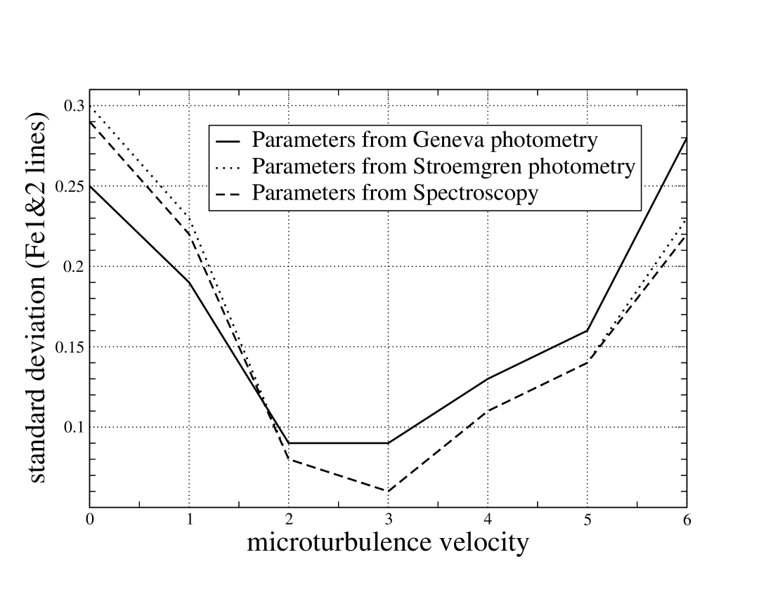
Figure 1: Standard deviation for Fe i and Fe ii lines, selected for HD 73730, as a function of $\upsilon_{\mathrm{mic}}$  using fundamental parameters obtained from Geneva photometry (straight line), from Strömgren photometry (dotted line) and from spectroscopy (dashed line).

For faster rotators an insufficient number of unblended lines are available with which to calculate the equivalent width. The more slowly-rotating Am stars of the sample show a mean $\upsilon_{\mathrm{mic}}$  value around 2.7 $\mathrm{km\,s}^{-1}$. For this reason, for fast rotators, we retained the value found using Eq. (1), which was always compatible, within the errors, with 2.7 $\mathrm{km\,s}^{-1}$.

Following Landstreet (1998) it has been generally adopted that for Am stars $\upsilon_{\mathrm{mic}}$  is between 4–5 $\mathrm{km\,s}^{-1}$. By contrast in the present work we determined values between 2.3–3.1 $\mathrm{km\,s}^{-1}$, for the slowly rotating stars.

The chemical elements used to determine the fundamental parameters were different for each star, depending mainly on the value of ${\upsilon}\sin i$, and are described in Sect. 5.

For the lines used to eliminate the correlations discussed above we assumed that non-LTE and stratification effects were negligible (Ryabchikova et al. 2007).

The wavelength range of the ESPaDOnS  orders was wide enough to perform a safe continuum normalisation of the H$\alpha$ and H$\beta$ lines. For the spectra obtained with this instrument it was therefore possible to use these two hydrogen lines to provide an additional constraint on the fundamental parameters. In particular, for effective temperatures less than 8000 K, the wings of the Hydrogen lines are very sensitive to the effective temperature. On the other hand, at higher effective temperatures the wings are particularly sensitive to $\log g$. We did not use the hydrogen lines of the spectra obtained with ELODIE and MuSiCoS because the wavelength ranges of the orders containing the H$\alpha$ and H$\beta$ lines were too narrow to include the entire line profile.

The spectroscopic procedure of refining the fundamental parameters reduces the errors of $T_{\mathrm{eff}}$ and $\log g$ to typically 200 K and 0.2, respectively, while the estimated error for $\upsilon_{\mathrm{mic}}$ is around 0.2 $\mathrm{km\,s}^{-1}$. These errors are estimated taking into account different noise sources, including continuum normalisation errors and uncertainty in the convective model. The errors associated with the effective temperature and $\log g$  have been confirmed by a fit of the H$\alpha$ and H$\beta$ line profiles using the models calculated with the parameters obtained from the estimated errors.

In some cases a star’s high rotational velocity prevented us from recovering $T_{\mathrm{eff}}$  and $\log g$  spectroscopically with good precision. In these cases we ultimately adopted an average of parameters determined spectroscopically and those obtained via Strömgren photometry.

For the spectra obtained with the ELODIE spectrograph we also attempted to check for the presence of a magnetic field by looking for a correlation between the abundance derived from each line and its Landé factor. We also conducted a search for magnetically-split lines (e.g. Fe ii line at 6149.258 Å) in spectra of the very slowest rotators. In fact, for ${\upsilon}\sin i$  more than a few $\mathrm{km\,s}^{-1}$  this method cannot be used for detecting typical Ap-star magnetic fields. For the spectra obtained with the ESPaDOnS  spectrograph we used the LSD technique to measure the velocity-resolved Stokes $V$ profile and the longitudinal magnetic field.

With the correct fundamental parameters, we determined the best value of ${\upsilon}\sin i$  fitting it on the Fe i lines at 5434.524 Å  and 5576.089 Å. We chose these two Fe i lines because their broadening parameters are well known and are not affected by magnetic field broadening, since their Landé factor is close to $0$. The estimated error on ${\upsilon}\sin i$  is about 5%.

The radial velocity, in $\mathrm{km\,s}^{-1}$, was determined by performing the median of the results obtained by fitting several lines of the observed spectrum to a synthetic one.

4.3 Element abundance analysis

Once we had obtained the best values for the fundamental parameters, we determined the final elemental abundances by direct fitting of the observed spectra with synthetic models. We synthesised the model spectra with Synth3 (Kochukhov 2006) and fit the cores of selected lines to get a value of the abundance associated with each line. We then calculated the mean and the relative standard deviation for each analysed element. The line core fitting was performed with the ’Lispan’ and ’ATC’ codes (written by Ch. Stütz) together with Synth3. The only free parameter in the line core fitting procedure is the abundance of the line. The fitting procedure and the determination of the abundances was performed iteratively in order to obtained a better determination of the abundances for blended lines. The error associated with the derived abundance of each element is the standard deviation from the mean abundance of the selected lines of that element. These errors do not take into account the uncertainties of the fundamental parameters and of the adopted model atmosphere. To have an idea of these uncerteinties, we have calculated the abundances of Fe, Ti and Ni for HD 73730 with five different models varing $T_{\mathrm{eff}}$  of $\pm$200 K and $\log g$  of $\pm$0.2 dex from the adopted model. We found a variation of less than 0.2 dex for Fe, 0.1 dex for Ti and 0.1 for Ni due to the temperature varation. We did not find any significant abundance change varing $\log g$. The uncertainty in temperature is probably the main error source on our abundances.

The lines used to synthesise the spectra and selected to calculate the abundances for the various elements were extracted from the VALD database.

The number of selected lines depends on the ${\upsilon}\sin i$  value found for each star. We also checked the log$gf$  value of each selected line using the solar spectrum. Lines in the synthetic spectrum of the Sun showing large deviations from the observed solar spectrum were rejected from the selection. For some elements (e.g. Co, Cu and Zn) we derived the abundance from one line. This does not mean that only one line is present in the spectrum, but that only one line was selected to derive the chemical abundance. Other lines of the same element are present, but they were not selected because they are either too much blended or their log$gf$  value appeared to be in error based on the solar spectrum.

For the elements which were not analysed we assumed solar abundances from Asplund et al. (2005).

4.4 Non-LTE effects

Some potassium lines were visible in the ESPaDOnS spectra (because of the extension of the spectra into the far red), making possible the calculation of the abundance of this element. In particular the K i line at 7698.974 Å was detected and was largely unblended in the spectra of most stars. Unfortunately, this element presents strong non-LTE effects; for this reason the K abundances derived here are reported only as upper limits. The He, O and Na lines were selected in such a way to reduce as much as possible non-LTE  effects. For He, we selected lines in the blue region; for O, lines in the red region; and for Na, we used the Na i doublet at $5682.633-5688.205$ Å, which is known to be essentially uneffected by non-LTE  effects (Ryabchikova, private communication). For all the other elements that present important non-LTE effects (e.g. C, N, Al, S, Y, Ba), the abundances derived here should be considered as upper limits (Baumueller & Gehren 1997; Kamp et al. 2001; Przybilla et al. 2006, and references therein). However at present day it is not known how large are the deviations from LTE for normal A-type stars and Am stars for the various elements. More non-LTE  analysis should be performed for this type of star. Since our sample of stars has similar fundamental parameters (mainly $\log g$  and metallicity) the non-LTE  effects associated to each star should be of the same magnitude. This allows us to compare the stars of our sample with each other.

5 Results

We have organised our sample of program stars according to their literature classification as normal A-type stars (HD 73430, HD 73575), Blue Stragglers (HD 73666 – Ap(Si) star) and Am stars (HD 72942, HD 73045, HD 73730, HD 73618, HD 73174, HD 73711, HD 73818, HD 73709).

Table 2 lists the initial and final set of fundamental parameters obtained for each program star.

Table 2: Initial and final atmospheric fundamental parameters for the analysed stars of the Praesepe cluster. The initial fundamental parameters are derived from photometry, the final with spectroscopy. The errors on the fundamental parameters are estimated to be 200 K, 0.2 $\mathrm{km\,s}^{-1}$and 0.2 for $T_{\mathrm{eff}}$, $\upsilon_{\mathrm{mic}}$  and $\log g$  respectively. The estimated error on ${\upsilon}\sin i$  is about 5%. The ${\upsilon}_{\mathrm{r}}$  is given in $\mathrm{km\,s}^{-1}$. $\langle B_{z}\rangle$ indicate the Longitudinal Magnetic Field (measured in Gauss) calculated with the LSD tecnique. BS: Blue Straggler.

	initial set			final set
HD	$T_{\mathrm{eff}}$	$\log g$	$\upsilon_{\mathrm{mic}}$	$T_{\mathrm{eff}}$	$\log g$	$\upsilon_{\mathrm{mic}}$	$\upsilon_{\mathrm{macro}}$	${\upsilon}\sin i$	${\upsilon}_{\mathrm{r}}$	$\langle B_{z}\rangle$	comments
	[K]	[cgs]	[$\mathrm{km\,s}^{-1}$]	[K]	[cgs]	[$\mathrm{km\,s}^{-1}$]	[$\mathrm{km\,s}^{-1}$]	[$\mathrm{km\,s}^{-1}$]	[$\mathrm{km\,s}^{-1}$]	G
73430	7790	3.95	2.6	7660	4.02	2.6	0	73	33.7	1 $\pm$ 45	normal
73575	7435	3.46	2.7	7300	2.92	2.7	0	127	33.4	-215 $\pm$ 149	normal
73666	9429	3.84	2.2	9382	3.78	1.9	0	10	34.1	6 $\pm$ 5	SB1; BS; close to normal
72942	8237	3.80	2.5	8450	3.90	2.4	0	73	39.9	12 $\pm$ 31	SB?; between normal & Am
73045	7470	4.09	2.7	7570	4.05	3.6	10	10	27.9	-1 $\pm$ 4	SB1; Am
73730	8009	3.83	2.5	8070	3.97	2.6	0	29	36.6	-12 $\pm$ 9	Am
73618	8091	3.81	2.5	8170	4.00	2.5	0	47	15.1	$-$	SB1; Am
73174	7600	4.20	2.0	8350	4.15	2.9	0	$<$5	2.9	$-$	SB1; Am
73711	8269	3.95	2.5	8020	3.69	2.5	0	62	23.4	$-$	SB1; Am
73818	7232	3.82	2.8	7232	3.82	2.8	0	66	22.5	$-$	SB1; Am
73709	8063	3.79	2.5	8070	3.78	2.3	0	10	26.7	$-$	SB1; Am

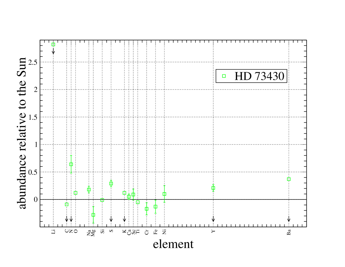
Figure 13: Elemental abundances relative to the Sun for HD 73430. The solar abundances are taken from Asplund et al. (2005). Arrows show elements affected by non-LTE  effects. Errors are given in Table3.

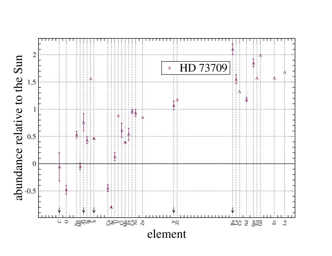
Figure 22: As for Fig. 13 for HD 73709

The derived abundances are illustrated in Fig. 13 to Fig. 22, and reported in Table 3.

Table 3: Abundances ($\log(N_{X}/N_{tot})$) of the program stars with the estimated internal errors in units of 0.01 dex, in parenthesis. For comparison, the solar abundances (Asplund et al. 2005) are given in the last column. At.N. gives the Atomic Numbers of the elements. Abundances obtained from just one line have no error ($-$). Upper limits are denoted by $<$.

		”Normal” A-type stars		Blue Straggler	Am stars								Solar
At.N.	Element	HD 73430	HD 73575	HD 73666	HD 72942	HD 73045	HD 73730	HD 73618	HD 73174	HD 73711	HD 73818	HD 73709	Abundances
2	He			$-1.20(05)$									$-1.11$
3	Li	$<-8.17(-)$	$<-8.50(-)$		$<-8.49(-)$	$-8.86(02)$	$-8.74(-)$	$<-8.58(-)$	$-8.51(02)$	$<-8.43(-)$	$<-8.63(-)$		$-10.99$
6	C	$<-3.74(-)$	$<-3.61(-)$	$<-3.25(03)$	$<-3.85(-)$	$<-4.37(04)$	$<-4.32(47)$	$<-4.16(16)$	$<-4.08(06)$	$<-3.99(15)$	$<-3.38(07)$	$<-3.71(26)$	$-3.65$
7	N	$<-3.62(16)$	$<-3.93(-)$	$<-3.67(10)$	$<-3.84(-)$	$<-4.49(-)$	$<-4.63(-)$		$<-4.50(12)$				$-4.26$
8	O	$-3.26(-)$	$-3.37(-)$	$-3.06(07)$	$-3.58(-)$	$-3.90(10)$	$-3.96(09)$	$-3.65(04)$	$-3.72(01)$	$-3.60(04)$	$-3.76(-)$	$-3.86(08)$	$-3.38$
11	Na	$-5.69(06)$		$-5.47(01)$		$-5.32(03)$	$-5.36(01)$	$-5.34(03)$	$-5.13(04)$		$-5.35(01)$	$-5.34(06)$	$-5.87$
12	Mg	$-4.79(15)$	$-4.63(-)$	$-4.25(14)$	$-4.51(03)$	$-4.52(04)$	$-4.43(06)$	$-4.29(-)$	$-4.21(05)$	$-4.63(05)$	$-4.51(16)$	$-4.56(06)$	$-4.51$
13	Al			$<-5.34(06)$		$<-5.41(01)$	$<-5.37(-)$		$<-5.06(-)$			$<-4.91(16)$	$-5.67$
14	Si	$-4.44(04)$	$-4.41(-)$	$-4.30(01)$	$-4.67(-)$	$-4.21(05)$	$-4.21(05)$	$-4.51(-)$	$-4.08(11)$	$-4.19(05)$	$-3.44(32)$	$-4.10(06)$	$-4.53$
15	P								$-5.23(-)$			$-5.12(-)$	$-6.68$
16	S	$<-4.59(-)$		$<-4.47(-)$	$<-4.48(-)$	$<-4.67(09)$	$<-4.54(03)$	$<-4.52(13)$	$<-4.37(03)$	$<-4.62(-)$	$<-4.36(26)$	$<-4.44(01)$	$-4.90$
18	Ar			$-5.10(-)$									$-5.86$
19	K	$<-6.84(-)$	$<-6.46(-)$	$<-6.49(-)$		$<-7.04(-)$	$<-6.83(-)$						$-6.96$
20	Ca	$-5.68(05)$	$-5.55(08)$	$-5.53(14)$	$-5.58(12)$	$-6.46(04)$	$-6.36(03)$	$-5.74(07)$	$-5.70(08)$	$-5.95(08)$	$-5.88(03)$	$-6.18(06)$	$-5.73$
21	Sc	$-8.90(10)$	$-9.31(10)$	$-8.95(06)$	$-8.88(11)$	$-9.39(01)$	$-9.71(03)$	$-9.51(27)$	$-9.44(08)$	$-10.06(01)$	$-10.90(-)$	$-9.79(01)$	$-8.99$
22	Ti	$-7.19(-)$	$-7.18(-)$	$-6.86(04)$	$-6.89(07)$	$-6.95(04)$	$-6.99(09)$	$-6.41(01)$	$-6.72(05)$	$-7.08(04)$	$-6.81(30)$	$-7.01(07)$	$-7.14$
23	V			$-7.48(05)$		$-7.60(-)$			$-7.19(05)$			$-7.16(-)$	$-8.04$
24	Cr	$-6.57(11)$	$-6.29(-)$	$-6.01(07)$	$-6.41(16)$	$-5.63(16)$	$-5.65(08)$	$-5.93(10)$	$-5.69(08)$	$-6.08(09)$	$-6.23(-)$	$-5.79(13)$	$-6.40$
25	Mn			$-6.32(01)$	$-6.91(-)$	$-6.28(-)$	$-6.31(03)$	$-6.28(-)$	$-6.07(06)$	$-6.46(13)$	$-5.83(-)$	$-6.26(01)$	$-6.65$
26	Fe	$-4.72(12)$	$-4.75(10)$	$-4.30(07)$	$-4.47(07)$	$-4.03(04)$	$-4.14(05)$	$-4.13(10)$	$-3.88(09)$	$-4.44(13)$	$-4.26(20)$	$-4.05(11)$	$-4.59$
27	Co					$-6.47(04)$	$-6.15(-)$		$-6.12(12)$			$-6.16(04)$	$-7.12$
28	Ni	$-5.71(15)$	$-5.56(01)$	$-5.53(03)$	$-5.57(-)$	$-4.93(06)$	$-5.14(07)$	$-5.10(15)$	$-4.79(02)$	$-5.28(02)$	$-5.32(14)$	$-4.88(06)$	$-5.81$
29	Cu					$-6.93(-)$	$-7.12(-)$		$-6.78(-)$		$-7.29(-)$		$-7.83$
30	Zn					$-6.65(-)$	$-6.82(-)$	$-7.29(-)$	$-6.42(-)$			$-6.59(-)$	$-7.44$
39	Y	$<-9.62(06)$		$<-9.78(-)$	$<-9.02(16)$	$<-8.91(09)$	$<-8.98(05)$	$<-8.62(-)$	$<-8.50(09)$	$<-8.77(13)$	$<-9.42(29)$	$<-8.76(08)$	$-9.83$
40	Zr					$-9.05(01)$	$-8.51(01)$		$-8.16(03)$			$-8.28(-)$	$-9.45$
56	Ba	$<-9.47(-)$	$<-9.95(-)$	$<-9.13(04)$	$<-8.97(-)$	$<-8.50(-)$	$<-7.85(16)$	$<-8.09(18)$	$<-8.02(38)$	$<-8.97(09)$	$<-8.69(06)$	$<-7.77(10)$	$-9.87$
57	La					$-9.61(09)$	$-9.41(-)$		$-9.26(09)$			$-9.36(08)$	$-10.91$
58	Ce					$-9.26(04)$	$-9.44(03)$		$-8.94(15)$			$-9.14(-)$	$-10.46$
59	Pr								$-9.09(-)$				$-11.33$
60	Nd					$-9.48(03)$	$-9.66(11)$		$-9.23(07)$			$-9.41(04)$	$-10.59$
62	Sm					$-9.89(05)$			$-9.81(10)$			$-9.18(07)$	$-11.03$
63	Eu					$-10.20(-)$	$-10.42(-)$					$-9.95(-)$	$-11.52$
64	Gd								$-9.30(04)$			$-8.93(-)$	$-10.92$
68	Er					$-9.65(-)$			$-9.39(-)$			$-9.54(-)$	$-11.11$
70	Yb					$-9.87(-)$							$-10.96$
71	Lu								$-10.20(-)$			$-10.3(-)$	$-11.98$
	$T_{\mathrm{eff}}$	7660	7300	9382	8450	7570	8070	8170	8350	8020	7232	8070
	$\log g$	4.02	2.92	3.78	3.90	4.05	3.97	4.00	4.15	3.69	3.82	3.78
	$\upsilon_{\mathrm{mic}}$	2.6	2.7	1.9	2.4	3.6	2.6	2.5	2.9	2.5	2.8	2.3
	$\upsilon_{\mathrm{macro}}$	0.0	0.0	0.0	0.0	10.0	0.0	0.0	0.0	0.0	0.0	0.0
	${\upsilon}\sin i$	73	127	10	73	10	29	47	$<$5	62	66	10

In the following sections we comment on individual stars, devoting special attention to the elements that characterise the peculiarities of each star.

5.1 Normal A-type stars

5.1.1 HD 73430

This is the slower rotator (${\upsilon}\sin i$ = 73 $\mathrm{km\,s}^{-1}$) of the two normal A-type stars studied. The LSD profile (Fig. 2) shows symmetric rotational broadening, and does not show any particular features; the analysis gives a longitudinal magnetic field of $\langle B_{z}\rangle=1\pm 45$ G.

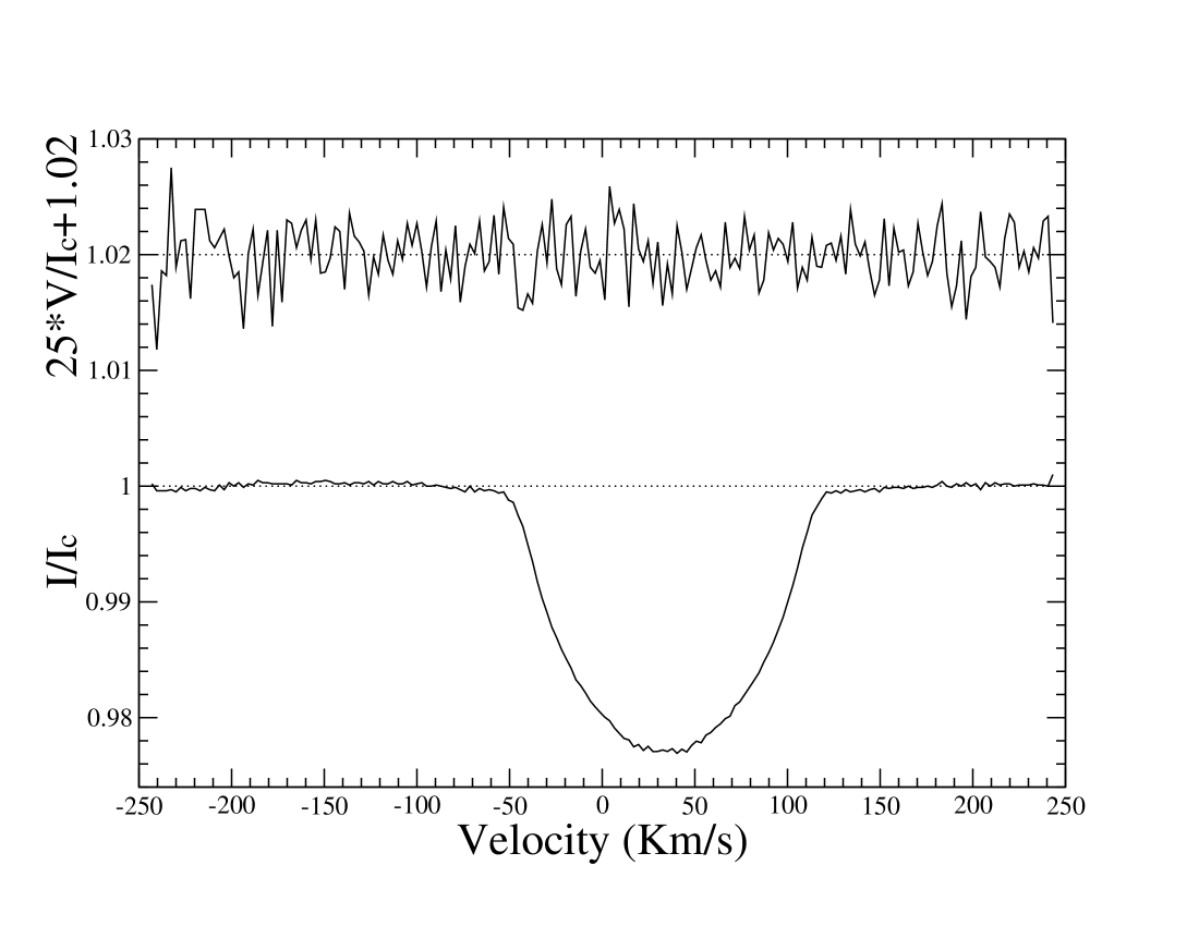
Figure 2: LSD profiles for the normalised Stokes $I$ and Stokes $V$ spectra (from bottom to top) of HD 73430. The Stokes $V$ profile is expanded by a factor of 25 and shifted upward of 1.02.

The effective temperature was determined so as to cancel any dependence of abundance versus excitation potential for Fe i. The $\log g$  was calculated imposing equilibrium between the Fe i and Fe ii abundances. The values for $T_{\mathrm{eff}}$ and $\log g$  found in this way were then averaged with the values found with the photometry. The $T_{\mathrm{eff}}$ was then checked and found consistent with the H$\alpha$ and H$\beta$ profiles, very sensitive to effective temperature at $T_{\mathrm{eff}}$ $<$ 8000 K.

We find that C and O are solar and N is overabundant, as is observed for the other normal A-type star of our sample, HD 73575 (see Sect. 5.1.2). This differs from the Am stars, in which these elements are usually observed to be underabundant. We note that Asplund et al. (2005) have significantly reduced the solar abundances of C, N and O, so all comparisons with the Sun of previous A-star studies regarding these elements may need to be revised. Ca, Sc, Ti, Cr, Fe and Ni are solar within the errors, allowing us to confirm the previous classification of HD 73430 as a normal A-type star.

5.1.2 HD 73575

This is the faster rotator (${\upsilon}\sin i$  = 127 $\mathrm{km\,s}^{-1}$) of the two normal A-type stars. HD 73575 is present in the catalog of Rodriguez et al. (2000) of $\delta$ Scuti variable stars. The Stokes $I$ LSD profile (Fig. 3) shows remarkable structure that may well be due to pulsation. No magnetic field was detected ($\langle B_{z}\rangle=-215\pm 149$ G).

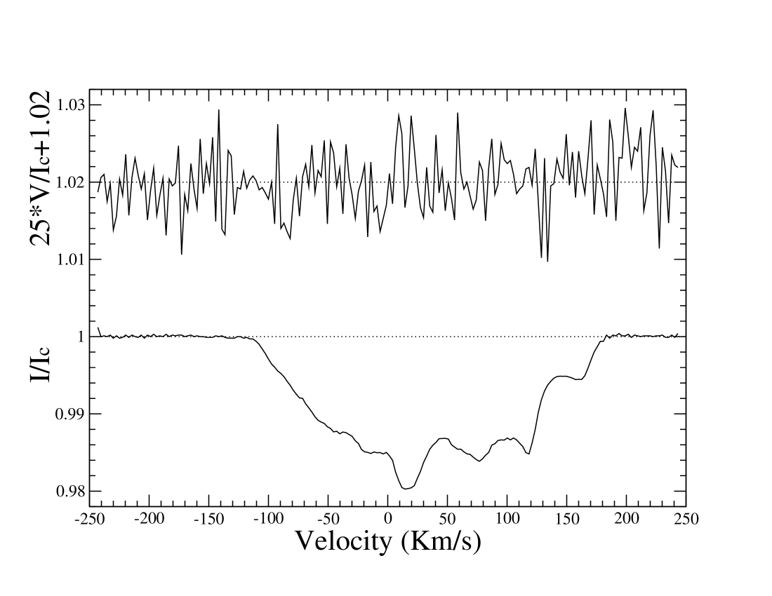
Figure 3: LSD profiles for the normalised Stokes $I$ and $V$ (from bottom to top) spectra of the $\delta$ Scuti star HD 73575. The Stokes $V$ profile is expanded by a factor of 25 and shifted upward of 1.02.

The very high ${\upsilon}\sin i$  resulted in a relatively small number of metal lines with which to tune the fundamental parameters. The effective temperature was also determined by fitting the H$\alpha$ and H$\beta$ line profiles, which were then combined with the values obtained with the photometry. The $\log g$  was determined by imposing equilibrium between different ionisation stages (Fe i and Fe ii). Due to the very high rotational velocity, the errors on the fundamental parameters are estimated to be similar to the photometric ones.

HD 73575 shows all the properties of normal A-type stars of the cluster (e.g. C and O solar with N overabundant; Fe underabundant), except for Sc, which appears to be slightly underabundant.

5.2 The Blue Straggler HD 73666

HD 73666 is the hottest star of the sample and the only Blue Straggler present in the cluster, according to Andrievsky (1998). It is also included in the ”New Catalogue of Blue Stragglers in Open Clusters” by Ahumada & Lapasset (2007). The photospheric chemistry of this star has been previously investigated by several authors (Andrievsky 1998; Burkhart & Coupry 1998), but their results, the iron abundances for example, vary wildly ([Fe/H] = $+0.1$, $+0.5$ respectively). These discrepancies are probably due to the narrow wavelength ranges available to those investigators.

The result of the application of the LSD technique is shown in Fig. 4.

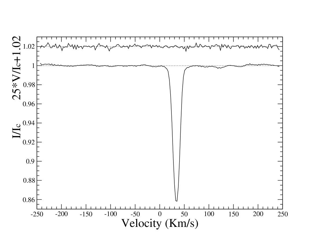
Figure 4: LSD profiles for the normalised Stokes $I$ and $V$ (from bottom to top) spectra for the Blue Straggler HD 73666. The Stokes $V$ profile is expanded by a factor of 25 and shifted upward of 1.02.

The derived longitudinal magnetic field is $\langle B_{z}\rangle=6\pm 5$ G.

This star is the primary component of a close binary system (SB1), as is the case for many other Blue Stragglers (Leonard 1996), and the flux coming from the secondary star is negligible, as previously checked by Burkhart & Coupry (1998), so the star was analysed ignoring the presence of the secondary.

The sharp lines (${\upsilon}\sin i$  = 10 $\mathrm{km\,s}^{-1}$) allowed for a detailed abundance analysis. The microturbulence velocity and $T_{\mathrm{eff}}$ were determined respectively by eliminating the abundance–equivalent width and abundance–excitation potential correlations, using Fe i, Fe ii and Ti ii lines. The $\log g$ value was obtained using the equilibrium between Fe i and Fe ii, and finally by looking for the best fit of the profile for the H$\alpha$ and H$\beta$ line wings (very sensitive to $\log g$  at $T_{\mathrm{eff}}$  $>$ 8000K). The resulting $\log g$ is the average of the values obtained with the two methods.

For the adopted model, Mg i and Mg ii deviate noticeably from the ionisation equilibrium condition. Their abundances are $-3.98$ and $-4.35$ respectively. The same behavior was found for Ca i and Ca ii with abundances of $-5.65$ and $-5.41$ respectively. These features of the Mg and Ca abundances explain the high value of the associated errors.

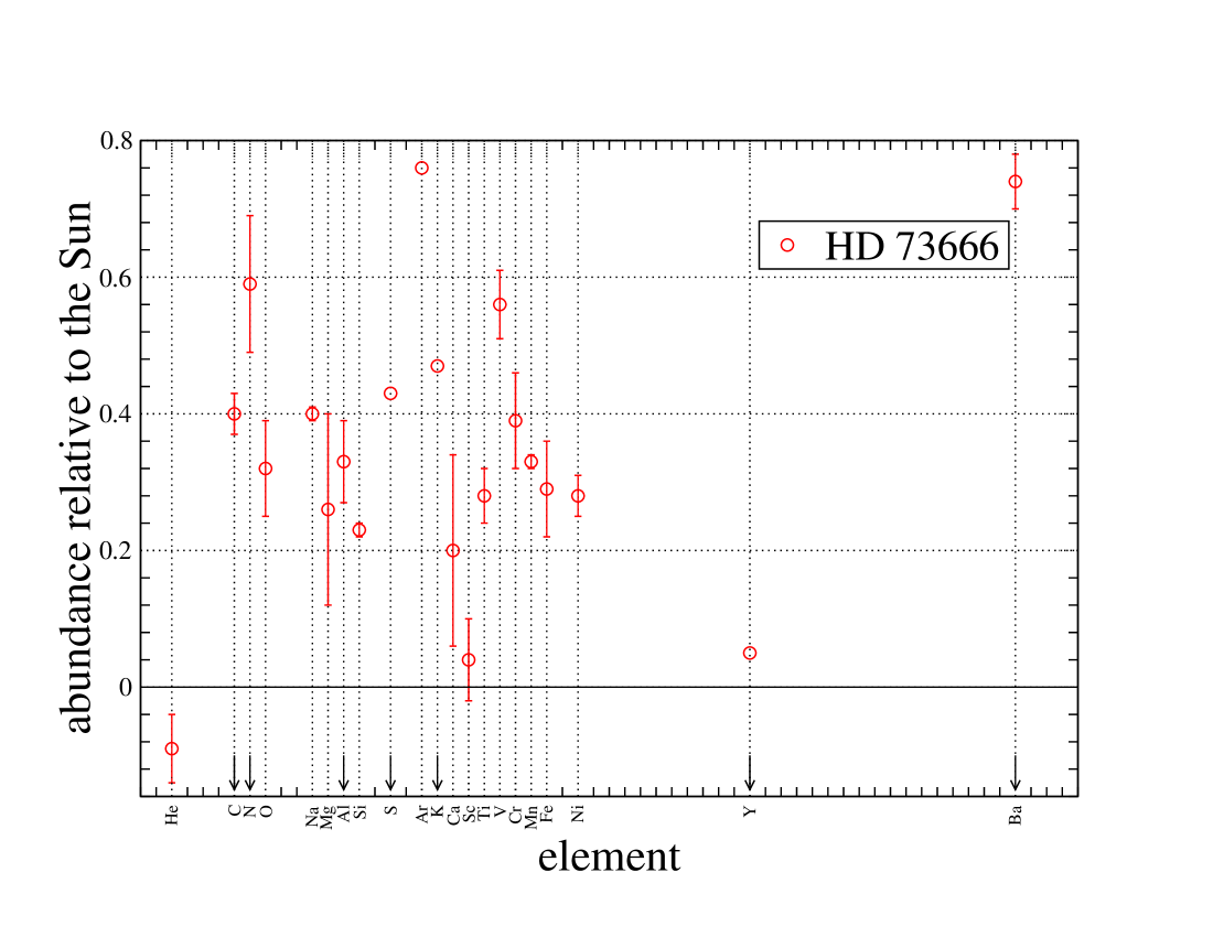
Figure 15: As for Fig. 13 for HD 73666

Abt (1985) classified this star as Ap (Si). The signature of this kind of star is a strong silicon overabundance. However, it can be seen in Table 3 and Fig. 15 that the Si abundance is not much higher than the solar abundance of this element. Also Ap (Si) stars are magnetic, and the very high precision of the longitudinal field diagnosis effectively rules out the presence of any organised magnetic field. Fig. 5 shows one of the selected Si lines. If HD 73666 was an Ap(Si) star, we would expect this line to be much stronger, compared to the surrounding Fe lines.

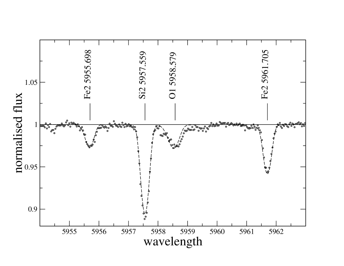
Figure 5: Portion of the spectrum of HD 73666. The dots show the observation, the dashed line shows the synthetic spectrum. The weak blended lines are omitted.

Andrievsky (1998) cataloged this star as an Am star, but Ca is slightly overabundant while Sc is solar. C, N and O are overabundant and, as it is possible to see in Fig. 10, these overabundances are typical of the normal A-type stars of the Praesepe cluster. These results allow us to conclude that HD 73666 is neither an Ap nor an Am star.

5.3 Am stars

In this section we analyse the stars of the sample classified as Am stars in previous works. According to Preston (1974) a star in the temperature range of 7000 – 10000 K is classified as Am (CP1) if Ca and/or Sc are underabundant and the heavy metals are overabundant. Am stars nearly always show low values of ${\upsilon}\sin i$, tipically less than 100 $\mathrm{km\,s}^{-1}$.

5.3.1 HD 72942

The LSD profile for HD 72942 is symmetric and rotationally broadened, as is illustrated in Fig. 6.

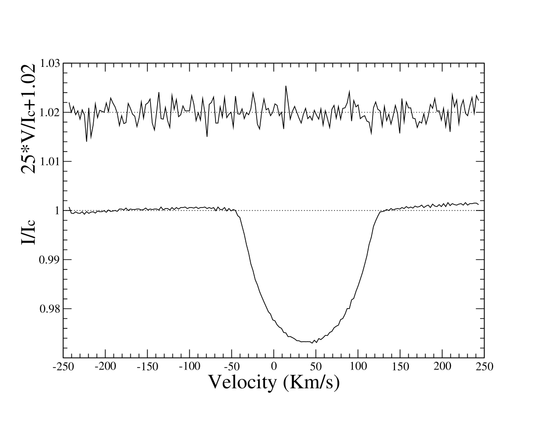
Figure 6: LSD profiles of the normalised Stokes $I$ and $V$ (from bottom to top) spectra of HD 72942. The Stokes $V$ profile is expanded by a factor of 25 and shifted upward of 1.02.

The magnetic analysis of the LSD profiles gives a value of the longitudinal magnetic field of $\langle B_{z}\rangle=12\pm 31$ G.

$T_{\mathrm{eff}}$ was set using Ti ii and Fe i lines. The $\log g$ value was estimated using the equilibrium between the Fe i and Fe ii abundances and fitting the H$\alpha$ and H$\beta$ line profiles.

The large error associated with the Y abundance is due to the poor determination of the line parameters and to the unknown non-LTE  effects associated with each line. It was not possible to derive the K abundance from the K i line at 7698.974 Å  because the line was blended by a telluric line.

Ca and Sc are not underabundant, indicating that HD 72942 is probably not an Am star. However, the Fe abundance is similar to that observed in the metallic stars of the sample.

HD 72942 is not known to be a spectroscopic binary and is neither a classical Am star nor a normal A-type star (Sect. 6.2). The calculated radial velocity is rather high as compared to those of the other members and to the mean of the cluster. See also the discussion in Sect. 6.2.

5.3.2 HD 73045

HD 73045 is the primary component of an SB1 binary system (Debernardi et al. 2000). It exhibits a low projected rotational velocity (${\upsilon}\sin i$  = 10 $\mathrm{km\,s}^{-1}$).

The LSD profiles of the Stokes $I$ and $V$ spectra are shown in Fig. 7.

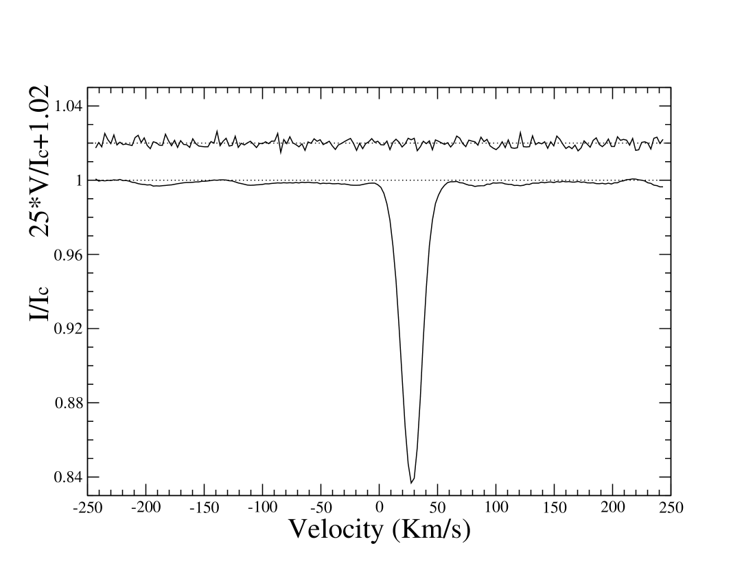
Figure 7: LSD profiles for the normalised Stokes $I$ and $V$ (from bottom to top) spectra of HD 73045. The Stokes $V$ profile is expanded by a factor of 25 and shifted upward of 1.02.

The magnetic field analysis provided a longitudinal magnetic field of $\langle B_{z}\rangle=-1\pm 4$ G.

The secondary star does not contribute significantly to the lines of the spectrum, according to Debernardi et al. (2000) and Budaj (1996), so we have analysed the system as a single star. During our abundance determination we noticed an extra broadening of the wings of deep lines, perhaps due to the binarity. To be able to fit these lines we introduced a macroturbulence velocity ($\upsilon_{\mathrm{macro}}$  = 10 $\mathrm{km\,s}^{-1}$  - obtained fitting several deep lines) to compensate for this effect. The use of the macroturbulence velocity does not lead to any significant abundance change, as expected. In particular the Iron abundance calculated without the use of the macroturbulence velocity results to be 0.01 dex lower than the final adopted one. The microturbulence velocity and the effective temperature were established using Fe i, Fe ii and Ni i unblended lines, using the method described previously. The $\log g$ value was obtained imposing the ionisation equilibrium condition for Fe. The determined $T_{\mathrm{eff}}$  was then checked with the H$\alpha$ and H$\beta$ line wings.

HD 73045 is a typical Am star as Ca and Sc are underabundant and the Fe-peak elements are overabundant, as are the rare earth elements. C, N and O are underabundant, typical of all the Am stars of the sample. For the Cu i line at 5105.537 Å, Co i line at 5342.695 Å and Co i line at 5352.045 Å we applied a hyperfine structure correction, but the ${\upsilon}\sin i$ was too high to produce any detectable difference in the line broadening.

5.3.3 HD 73730

HD 73730 is an Am star with an intermediate rotational velocity (${\upsilon}\sin i$ = 29 $\mathrm{km\,s}^{-1}$).

The LSD profiles for the Stokes $I$ and Stokes $V$ spectra are shown in Fig. 8.

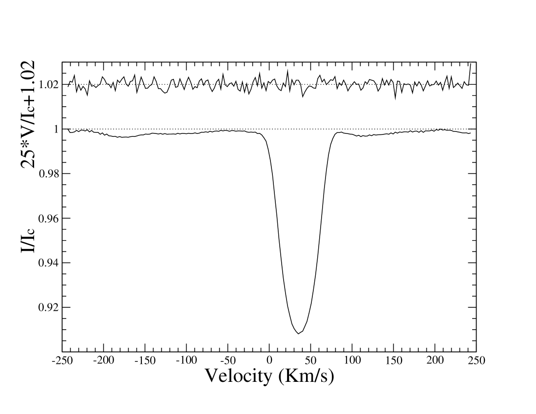
Figure 8: LSD profiles of the normalised Stokes $I$ and $V$ (from bottom to top) spectra of HD 73730. The Stokes $V$ profile is expanded by a factor of 25 and shifted upward of 1.02.

No magnetic field was detected from the LSD profiles. The calculated longitudinal magnetic field was $\langle B_{z}\rangle=-12\pm 9$ G.

We obtained the fundamental parameters ($\upsilon_{\mathrm{mic}}$, $T_{\mathrm{eff}}$, and $\log g$) using only Fe i and Fe ii lines, since the ${\upsilon}\sin i$ did not allow us to select a sufficient number of unblended lines with good line parameters for any other element. Since we had the possibility to use only Fe i and Fe ii lines, we also used the values of the $\log g$ obtained from the fitting of the H$\alpha$ and H$\beta$ line profiles.

The ${\upsilon}\sin i$ and the non-binarity allowed us to perform a precise abundance analysis for many elements - in fact only C shows a large error bar. This is probably due to the small number of selected C lines, all of which present non-LTE effects. The underabundances of Ca and Sc confirm that HD 73730 is an Am star. Also C, N and O are underabundant, as is the case for the other Am stars of the sample.

The ${\upsilon}\sin i$ is sufficiently large to hide any hyperfine structure broadening.

5.3.4 HD 73618

HD 73618 is the primary component of an SB1 binary system in which the flux of the secondary star does not significantly influence the total flux spectrum, according to Mason et al. (1993). For this star, as for all the others observed with the ELODIE spectrograph, we do not have a Stokes $V$ LSD profile since the instrument did not support a polarimetric mode. So we checked for the presence of a magnetic field with the correlation between abundance and Landé factor for Fe i. This method allows the detection of magnetic fields stronger than about 1–2 kG (Stütz et al. 2006). We did not find any detectable magnetic field for HD 73618. To obtain the $T_{\mathrm{eff}}$ and the $\log g$ we used Fe i and Fe ii lines. The fitting of the H$\alpha$ and H$\beta$ lines was not applied because their wings were broader than the wavelength range of the respective orders of the spectrograph. Since the ${\upsilon}\sin i$  is too high to get equivalent widths for enough unblended Fe i lines, we used the $\upsilon_{\mathrm{mic}}$  calculated with Eq. (1).

Only Sc is underabundant, while Ca is solar. C and O are underabundant, as we have found for the other Am stars of the sample. Also, the Fe-peak elements show a behavior typical of this type of star. This confirms the previous classification of HD 73618. Because of the lower resolution of the ELODIE spectrograph with respect to the ESPaDOnS spectrograph, the errors associated with the abundances turn out to be higher than those calculated for the other stars described above.

This star is included, as a Blue Straggler, in the catalogue by Ahumada & Lapasset (2007). Andrievsky (1998) analysed this star in his paper on Blue Stragglers in the Praesepe cluster, but he did not define it as a true Blue Straggler, since in the colour–magnitude diagram it does not lie outside the cluster’s main sequence. Our sample of stars is too small to allow us to generate a trustworthy colour–magnitude diagram based on spectroscopic temperatures. For this reason we are not able to confirm either the classification of Ahumada & Lapasset (2007) or that of Andrievsky (1998).

5.3.5 HD 73174

HD 73174 is the primary component of a triple SB1 system (Debernardi et al. 2000) and is the slowest rotator of the program stars, with ${\upsilon}\sin i$  $<$ 5 $\mathrm{km\,s}^{-1}$. The spectrum was obtained with the ELODIE spectrograph with a mean resolution of 45 000, not sufficient to allow an accurate measurement of the ${\upsilon}\sin i$ of this star.

Debernardi et al. (2000) obtained the masses of the three components of the system (2 M_☉; 0.68 M_☉; 0.63 M_☉). Knowing the age of the cluster (González-García et al. 2006, $\log(t)=8.85$) it was possible to estimate the effective temperatures and the radii of the three stars comprising the system. Using the evolutionary mass models of Schaller et al. (1992), we estimated the effective temperature and the radius of the primary component (8375 K and 2.22 R_☉ respectively). From plots on evolutionary models of cool stars of Gray (1992) we estimated the effective temperature and the radii of the other two components: 4557 K and 0.68 R_☉ for the secondary and 4300 K and 0.65 R_☉ for the third component. Since the presence of the third component is not certain we have not taken this star into account in our analysis. The radius ratio between the primary and the secondary star turns out to be $R_{1}/R_{2}$ = 3.26. We assumed a $\upsilon_{\mathrm{mic}}$  of 2 $\mathrm{km\,s}^{-1}$ for both the stars and a $\log g$  of 4.2 and of 4.4 for the primary and the secondary respectively. We calculated a model atmosphere for each of the two stars, using the parameters just described, and produced a synthetic spectrum for each of the two stars to check how much flux in the observed intensity spectrum is due to the secondary component. As it is possible to see in Fig. 9, the flux coming from the secondary star is negligible with respect to that of HD 73174. For this reason we analysed the system as a single one. The error bars on these inferred fundamental parameters could be very high since the error bars on the mass determination are unknown.

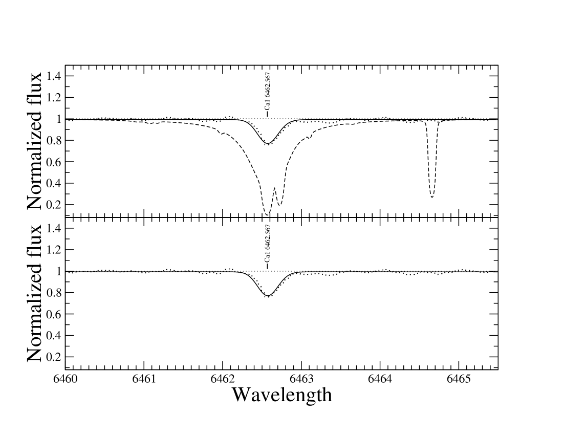
Figure 9: Comparison between the incoming flux from the two components of the HD 73174 system. In the upper panel the dotted thick line is the observed (normalised) spectrum, while the solid and the dashed lines are the synthetic spectra of the primary and the secondary star respectively. These two synthetic spectra are calculated with the parameters described in the text and with solar abundances. In the lower panel we show with the dotted thick line the observed and normalised spectrum and with the straight line the resultant synthetic spectrum after the application of the calculated radius ratio ($R_{1}/R_{2}$ = 3.26).

The low ${\upsilon}\sin i$ allowed us to perform a very detailed abundance analysis and the errors associated with the various elements are for this reason quite low, even if the signal to noise ratio and the resolution were not optimal.

C, N, O and Sc are underabundant while Ca is almost solar, as was found for HD 73618. For this reason we confirm the previous classification of this star. Only Ba shows a large error bar. This is probably due to the strong difference in depth of the selected lines and to the different influence that the non-LTE  effects have on each of these lines.

We took into account the hyperfine structure correction for the following lines: Co i at 5342.695 Å  and 5352.045 Å, Cu i at 5105.537 Å, Mn i at 6021.819 Å  and Zn i at 4722.153 Å. The abundance correction from HFS observed for all of these lines is smaller than 0.03 dex, much less than our typical errors.

We have to comment the difference of about 700 K between the $T_{\mathrm{eff}}$  derived from Strömgren photometry and from spectroscopy. We are not able to explain the reason for this dicrepancy. Probably, give concerning the very low ${\upsilon}\sin i$  of this star, a spectrum taken with a much higher resolution could solve this puzzle.

5.3.6 HD 73711

The ELODIE spectrum of this Am star has unfortunately a low SNR (Table 1) and a quite high ${\upsilon}\sin i$ (62 $\mathrm{km\,s}^{-1}$), making the abundance analysis more difficult and less precise. HD 73711 is also the primary component of an SB1 system. The abundances of this star were previously analysed by Burkhart & Coupry (1998) who considered the spectrum as that of a single star.

We have used Fe i and Fe ii lines to calculate the $T_{\mathrm{eff}}$ and $\log g$, while $\upsilon_{\mathrm{mic}}$ was calculated with Eq. (1). As with all the other ELODIE spectra we were not able to use the H$\alpha$ and H$\beta$ lines to determine the parameters. We have not found any detectable magnetic field with the abundance-Landé factor correlation for Fe i lines.

We confirm the previous classification of HD 73711, as Ca and Sc are underabundant, like C and O, as occurs for all the Am stars of the sample. The errors associated with the abundances are below 0.15 dex in spite of the high ${\upsilon}\sin i$ and the low SNR; only the error associated with the C abundance reaches 0.15 dex, probably due to the small number of selected lines used to calculate the final abundance, which were analysed without taking into account non-LTE effects.

5.3.7 HD 73818

The spectrum of the Am star HD 73818 has the lowest SNR of the whole sample. This fact, combined with the rather high ${\upsilon}\sin i$  (66 $\mathrm{km\,s}^{-1}$), made the abundance analysis very difficult and imprecise. This is the primary star of an SB1 system. We analysed this spectrum as a single star, as suggested by Burkhart & Coupry (1998).

We tried to calculate $T_{\mathrm{eff}}$ and $\log g$ using Fe i and Fe ii lines, applying the method described in Sect. 4.2, but we were never able to converge to two final values. For this reason we adopted the fundamental parameters calculated with the photometry. The $\upsilon_{\mathrm{mic}}$ was calculated using Eq. (1).

The abundances of many elements show large errors, mainly those elements for which non-LTE effects should be taken into account. The error associated with the Fe abundance is quite high in comparison to all other stars of the sample. This example illustrates the importance of a high SNR to be able to perform an accurate abundance analysis that starts with a spectroscopic determination of the fundamental parameters.

Ca and Sc are underabundant, confirming in this way the previous classification. Only the C abundance is higher than expected for an Am star of the Praesepe cluster.

5.3.8 HD 73709

HD 73709 is the primary star of an SB1 quadruple system (Abt & Willmarth 1999). The low ${\upsilon}\sin i$  allowed a good determination of the elemental abundances; only the moderate resolution of MUSICOS decreased the quality of our results.

This star was classified as Am by Gray & Garrison (1989), but was found photometrically to be an Ap star by Maitzen & Pavlovski (1987) according to the $\Delta a$ index ($\Delta a$ = $+0.018$ mag). Debernardi et al. (2000), using two ELODIE spectra and observations with the CORAVEL radial velocity scanner, found a magnetic field of 7.5 kG. Shorlin et al. (2002) looked for the presence of such a magnetic field using the LSD technique applied to the same MuSiCoS spectrum we analyse here. Their result shows clearly that HD 73709 does not have a significant magnetic field, with the measured value equal to $\langle B_{z}\rangle=66\pm 39$ G.

We calculated a synthetic $\Delta a$ value with respect to the theoretical normality line $a_{0}$ determined by Khan & Shulyak (2007, Sect. 3.3.2) and found that $\Delta a=+0.012$ mag, which is compatible with the observed value.

As mentioned before, this star is the main component of a quadruple system. We ruled out that the third or fourth components could contribute significantly to the light since they appear to be much less massive than the other components. The ratio between the masses of the primary and secondary component is $M_{2}/M_{1}$ $\geq$ 0.27 (Abt & Willmarth 1999). For HD 73174 we employed a value of $M_{2}/M_{1}$ $\geq$ 0.35 (Abt & Willmarth 1999) and in that case our test demonstrated that the flux coming from the secondary star was negligible with respect to the primary for a radius ratio lower than two (Sect. 5.3.5). For this reason we arrived immediately at the same conclusion as for HD 73174 - that the contribution of the secondary to the observed spectrum is negligible.

The $\upsilon_{\mathrm{mic}}$ and $T_{\mathrm{eff}}$ were established using Fe i, Fe ii and Ni i unblended lines. The $\log g$ was set imposing the ionisation equilibrium condition for Fe i and Fe ii. The fitting of the H$\alpha$ and H$\beta$ lines was not applied to obtained the fundamental parameters, for the same reason as for the ELODIE spectrograph.

O, Ca and Sc are underabundant, confirming in this way the previous classification. C and Al show large error bars ( $\geq$ 0.15 dex), probably due to the fact that non-LTE effects were not taken into account.

6 Discussion

6.1 Are weak magnetic fields present in the Am stars of Praesepe?

If magnetic fields are present in Am stars, this might help explain some of the peculiar properties of these stars, such as slow rotation and the typical Ca/Sc underabundances (Böhm-Vitense 2006).

We decided to use the LSD approach to detect magnetic fields in Am stars since this method is the most precise method currently available, especially for stars with rich line spectra and low ${\upsilon}\sin i$. As explained in Sect. 4.2 we have also looked for magnetic fields using other techniques, but these methods have resulted in substantially higher upper limits.

Lanz & Mathys (1993) have claimed evidence of magnetic fields in the Am star $o$ Peg ($T_{\mathrm{eff}}$  = 9550) using the difference of equivalent widths of two Fe ii lines at 6147.741 Å and 6149.258 Å. We did not try to apply the same method to compare our results to theirs as all of the sharp-lined Am stars in our sample are spectroscopic binaries, and the blending due to the spectral lines of the secondary might well affect the subtle signal of a magnetic field. Another problem is due to the fact that our Am stars are cool Am stars and the Fe ii line at 6147.741 Å is strongly blended by an Fe i line, preventing an accurate equivalent width determination.

Shorlin et al. (2002) analysed 25 Am stars with the LSD technique without finding any significant magnetic field signature. These authors concluded that no credible evidence exists for the presence of organised or complex magnetic fields in Am or normal A-type stars.

In our study, the three Am stars observed with ESPaDOnS and the one observed with MuSiCoS did not reveal any magnetic field signature in the circular polarized spectra, analysed with the LSD procedure. We also tried to detect the presence of potential magnetic fields in the other Am stars, observed with ELODIE, using the method described in Sect. 4.2. For all of them it was not possible to detect any magnetic field.

Our conclusion is that the cool Am stars of Praesepe ($T_{\mathrm{eff}}$ $<$ 8500 K) show no evidence of magnetic fields that could explain the well-known phenomena associated with Am stars. This result supports and strengthens the conclusion of Shorlin et al. (2002).

6.2 Normal vs. Am stars

In Fig. 10 and in Table 3 we show the final adopted abundances for all of the program stars.

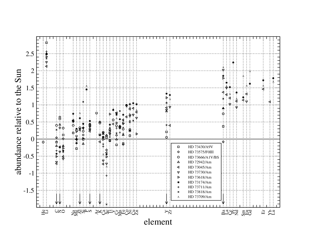
Figure 10: Elemental abundances relative to the Sun for the program stars. The solar abundances are taken from Asplund et al. (2005). In order to show a more readable Figure, the errors (Table 3) are omitted. Arrows show elements affected by non-LTE  effects.

The precision obtained with the abundance analysis allows us to distinguish two groups among the A-type stars of Praesepe: the normal A-type stars and the Am stars. For the two kinds of star analysed in this paper, the abundances of the Fe-peak elements are different. In normal A-type stars, Fe, Ni, and Cr are solar or slightly underabundant (compared to their solar abundances). In Am stars, these elements are slightly overabundant. In all but one of the stars of our sample, Ba is overabundant. However, the Ba abundance is definitely lower in normal A-type stars than in Am stars. This suggests that Ba may be considered as an additional indicator of Am peculiarities, together with C, N, O, Ca, Sc and the Fe-peak elements.

The abundance pattern found for HD 72942 deserves further comment. Bidelman (1956) classified HD 72942 as Am. Our abundance analysis shows some features common to the Am stars, like underabundances of C and O and an overabundance of Fe, and some others in common with normal A-type stars, like overabundance of N, Ca and Sc and a low Ba abundance. For these reasons we believe that HD 72942 has a chemical composition between the normal A-type stars and the Am stars. The high observed radial velocity of this star may be indicative of undetected binarity.

The remaining Am stars represent a fairly homogeneous sample.

6.3 Constraints to the diffusion theory

Underabundances of Sc and/or Ca and small overabundances of Iron-group elements are qualitatively explained by diffusion theory (see, e.g., the review in the introduction by Alecian (1996) and references therein). In particular, following Alecian (1996), Richer et al. (2000) developed a detailed modeling of the structure and evolution of Am/Fm stars, taking into account atomic diffusion of metals and radiative accelerations for all species in the OPAL opacities.

The results of this work can be used to constrain diffusion models, and we can compare our results with theoretical predictions. For the comparison, we use the abundances of HD 73730 (Fig. 11) since it is the star among those that are not binary with the lowest ${\upsilon}\sin i$, which favors the abundance analysis. Furthermore, the elemental abundances of this star are also representative of the homogeneous group of Am stars of the Praesepe cluster as listed in Sect. 6.2.

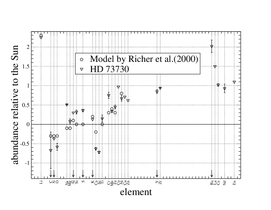
Figure 11: The open triangles show the abundances derived for HD 73730. The open circles show the predicted abundances displayed in Fig. 14 of Richer et al. (2000). Arrows show elements affected by non-LTE  effects

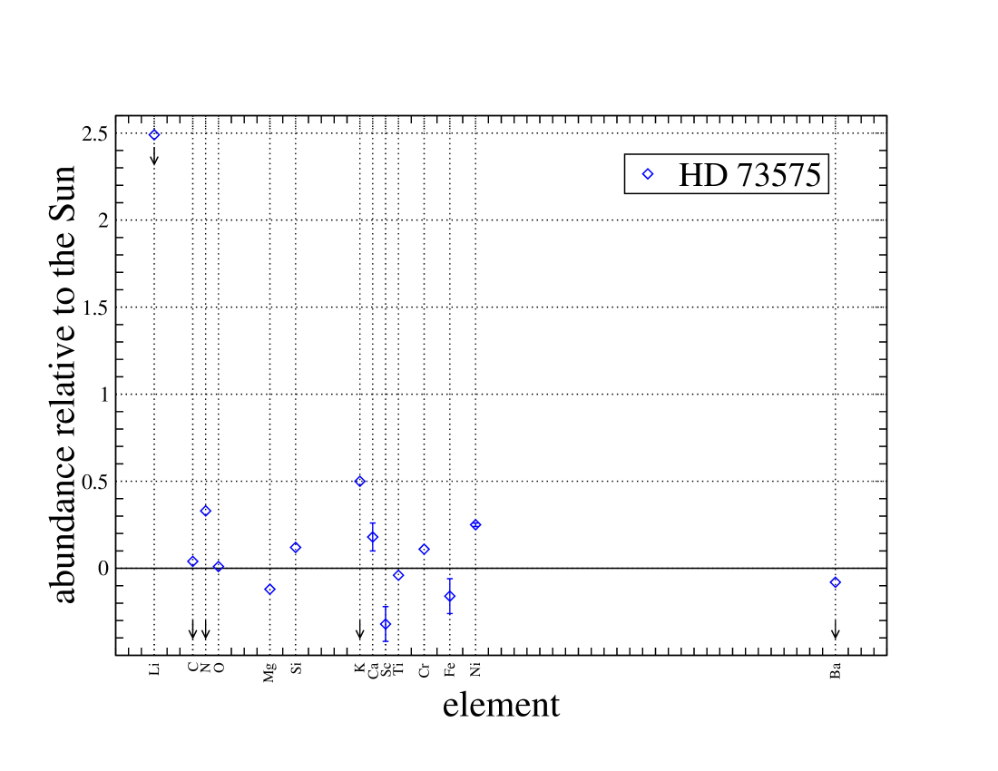
Figure 14: As for Fig. 13 for HD 73575

Figure 14 of Richer et al. (2000) shows the predicted abundances from a diffusion and turbulence model as a function of time and effective temperature. Open circles (reported also in Fig 11) refer to the predicted abundances for 670 Myr old stars, an age that is closely comparable to that one of the Praesepe cluster ($\sim$700 My, according to González-García et al. 2006). For temperatures around $T_{\mathrm{eff}}$ $=8000$ K, the temperature of HD 73730, the model by Richer et al. (2000) predicts underabundances of -0.3 (relative to the Sun) for C, N and O, of $-0.1$ for Na, Mg and Ca, solar abundances for Si, S and Ti, overabundances of $+0.1$ for Al, of $+0.3$ for Cr and Fe, of $+0.4$ for Mn, of $+0.8$ for Ni and $+2.3$ for Li, within 0.1 dex.

Our Fig. 10 (see also Table 3) shows an agreement for Li, C, N, O, Mg, Al, Si, Ca and Fe-peak elements within 0.1 dex. Discrepancies are apparent for Na and S (Sc was not modeled by Richer et al. (2000) because no OPAL data was available for Sc).

Na is the element for which the derived abundance ($\simeq 0.5$ dex with respect to the solar abundance) has the smallest scatter among the Am stars of our sample. Observations seems definitely to suggest an overabundance of this element which is inconsistent with model predictions of $-0.1$ dex.

S shows a small scatter in our sample ($\sigma$ = 0.12 dex). Kamp et al. (2001) analysed the S abundance in the metal poor A-type star $\lambda$ Boo in LTE and non-LTE. Their analysis shows that the S abundance determined in non-LTE  is lower than that determined in LTE by 0.1 dex. For metal poor stars non-LTE  effects are larger than for normal A-type stars and Am stars. This brings our S abundance ($\simeq+0.35$ dex) to an overabundance (relative to the Sun) of $\geq$0.25 dex, as compared with a solar abundance predicted by Richer et al. (2000). This apparent discrepancy should be investigated in non-LTE  regime.

6.4 Lithium abundance

In the context of radiative diffusion theory, it is interesting to examine the atmospheric abundance of lithium in stars where such a mechanism is known to be present, like in Am stars. Such studies have been carried out especially by Burkhart & Coupry (1991) and Burkhart et al. (2005). Their conclusion was that, in general, the Li abundance in Am stars is close to the cosmic value ($\log{N_{Li}/N_{total}}\sim-9.04$ dex), although a small proportion of them are Li deficient. The normal A-type stars appear to have a higher Li abundance ($\log{N_{Li}/N_{total}}\sim-8.64$ dex), in the $T_{\mathrm{eff}}$  range 7000–8500 K (Burkhart & Coupry 1995).

We have calculated precise Li abundances for HD 73045 and for HD 73174 taking into account hyperfine structure, while for HD 73730 we give an estimation derived from one line and without hyperfine structure. For other stars it was possible to derive only an upper limit, since the higher ${\upsilon}\sin i$  values did not allow a more accurate abundance determination. In HD 73666 we have not found any Li line, while for HD 73709 the MuSiCoS  spectrum did not cover the strong Li 6707.761 Å  line. Our determinations confirm the overabundances (relative to the Sun) for three Am stars. Since for the normal A-type stars and the other Am stars we can only derive upper limits, we cannot confirm the overabundances. In Fig. 12 we show the absolute Li abundance as a function of $T_{\mathrm{eff}}$, in comparison with the values given by Burkhart & Coupry (1995).

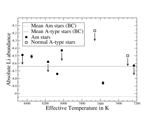
Figure 12: Distribution of the Li abundance as a function of the $T_{\mathrm{eff}}$. The dashed line shows the Li abundance value found by Burkhart & Coupry (1995) (BC in the legend) for normal A-type stars. The dotted line shows their Li abundance value for Am stars. The open squares and the closed circles correspond to the Li abundances of the program normal A-type stars and Am stars respectively. The upper limit values are indicated with an arrow.

Our sample is not large enough to address the behavior of the lithium abundance in the temperature range between 7000 K and 8500 K, but we notice that the abundances appear to be higher than those derived by Burkhart & Coupry (1995) in open clusters. We cannot confirm the tendancy of the normal A-type stars to have a higher Li abundance. Our results appear to be more consistent with those derived by North et al. (2007) for field stars.

6.5 Comparison with previous abundance determinations

In the past years, some of the stars belonging to our sample were analysed by different authors: Hui-Bon-Hoa et al. (1997), Hui-Bon-Hoa & Alecian (1998), Andrievsky (1998) and Burkhart & Coupry (1998).

In Table 4 (available only in the online version) we compare our final abundances with those obtained by other authors. The abundances coming from other papers were converted to our $\log{N_{{\rm el}}/N_{{\rm total}}}$ scale, using the solar abundances taken as reference in each paper.

As explained in Sect. 4.2, our $T_{\mathrm{eff}}$  and $\log g$  were determined spectroscopically, while the other authors derived these parameters from photometry. All the measurements are in perfect agreement considering the associated errors. This shows that for normal A-type stars and for Am stars the fundamental parameters, derived from photometry, are not too far from a more precise determination given by the spectroscopy. For some stars, the microturbulence velocity appears to differ for different authors. It is notable that the our $\upsilon_{\mathrm{mic}}$ and that derived by Hui-Bon-Hoa & Alecian (1998) for the slow rotator HD 73174 are in good agreement. This agreement is due probably to the similar methods used to derive it (see Hui-Bon-Hoa & Alecian 1998).

Taking into account a default error of 0.2 dex for the abundances without an individual error, inspection of Table 4 reveals a good agreement between our work and the previous ones. Only Li, Sc, Ba and Eu show some deviations. The deviation associated with the Sc abundance occurs because of the difficulty to calculate this abundance for Am stars in which Sc is underabundant, showing only shallow lines. Concerning the Ba and Eu discrepancies, they could be due to a different line selection with different non-LTE effects associated with the Ba lines and a different weight given to the blended Eu lines, selected to determine the abundances. We are not able to find a clear reason of the discrepancies for the Li abundances.

We believe that our determination of the fundamental parameters and of the elemental abundances are affected by smaller external errors than those of the other authors. We state this based on the wider wavelength range available, on the use of better and more carefully-checked line parameters, on the more reliable atmospheres models used and finally on the methodology used to determine the abundances (fitting of the line profile instead of using equivalent widths).

7 Conclusions

We have obtained high resolution, high SNR spectra for eleven A-type stars belonging to the nearby intermediate-age Praesepe open cluster. For seven stars of the sample the spectra were also obtained in circular polarization.

Eight stars of the sample were previously classified as Am stars, two as normal A-type stars and one as an Ap (Si) star. We have calculated the fundamental parameters and performed a detailed abundance analysis for each star of the sample. For the stars observed in circular polarization we have used the LSD technique to measure the longitudinal magnetic field.

No significant magnetic field signature was found applying the LSD technique to the Am stars, which were observed with ESPaDOnS and MuSiCoS. This leads us to the conclusion that peculiar abundances and slow rotation of the Praesepe Am stars cannot be explained by the presence of a magnetic field. But since nearly all of them are SBs we can conclude that slow rotation, induced by binarity, can lead to the Am chemical peculiarities.

Fundamental parameters and elemental abundances were derived by adjusting synthetic spectra to the observed ones. The model atmospheres were computed by means of the 8.4 version of the LLmodels code, without taking into account non-LTE corrections, using atomic line data extracted from the VALD database. Synthetic spectra were produced with Synth3 (Kochukhov 2006).

The abundance analysis shows that the Blue Straggler HD 73666, previously classified Ap (Si) star, is a normal A-type star. This star does not show any magnetic field nor peculiarity. We confirm the membership and the classification of the two normal A-type stars HD 73430 and HD 73575. HD 72942 cannot be confirmed either as member of the cluster or as an Am star. For all the other Am stars classification is confirmed.

For this sample of Am stars we have compared our abundances with the predictions of diffusion models by Richer et al. (2000). We obtained an excellent agreement, within the errors, with the predictions for almost all the common elements. Only Na and probably S show a clear discrepancy from the theoretical abundances. Unfortunately, our Na and S abundances do not take into account non-LTE effects that would bring the abundances closer to the predictions of theory (Kamp et al. 2001). A non-LTE abundance determination should be performed, at least for a few Am stars, in order to confirm the abundance predictions of these two elements. Richer et al. (2000) did not analyse Sc because it is not present in the OPAL opacity database. Model predictions for this element and for heavy elements are especially important and should be performed.

Finally, we have turned our attention to the Li abundance of the sample, obtaining results comparable to those of Burkhart & Coupry (1995), in open clusters, and North et al. (2007), for field stars.

Our results indicate that radiative diffusion, combined with turbulent mixing, can account for most of the chemical peculiarities found in Am stars. More abundance determinations on cluster stars with a variety of ages will help to constrain the physical processes at work in A and Am stars.

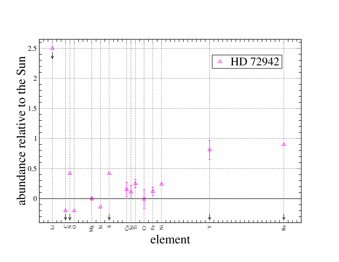
Figure 16: As for Fig. 13 for HD 72942

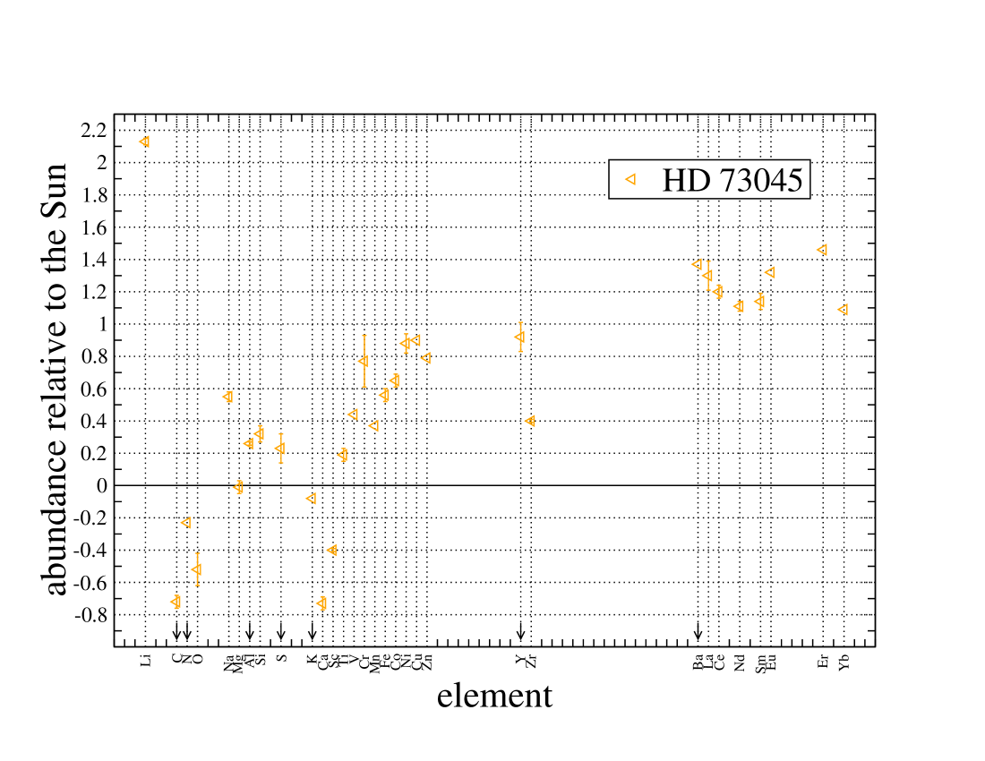
Figure 17: As for Fig. 13 for HD 73045

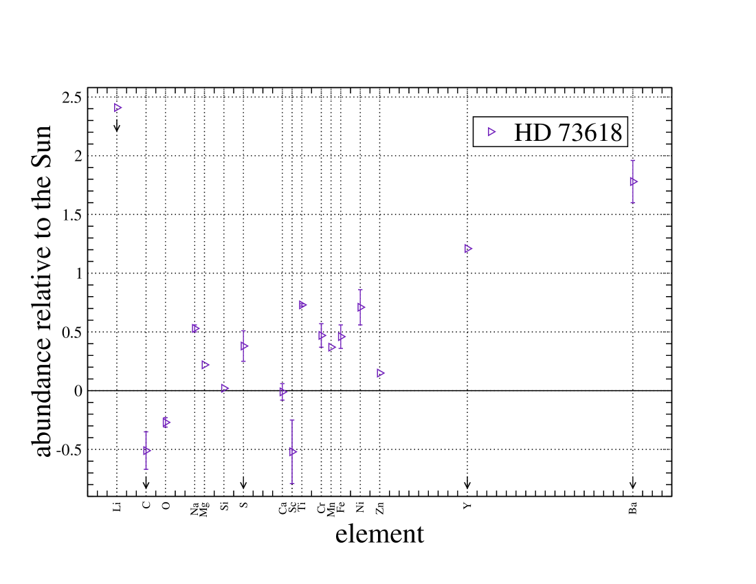
Figure 18: As for Fig. 13 for HD 73618

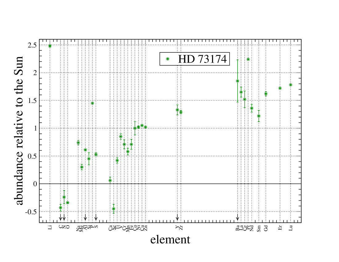
Figure 19: As for Fig. 13 for HD 73174

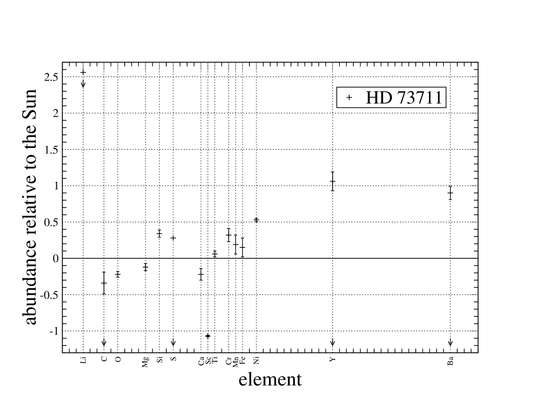
Figure 20: As for Fig. 13 for HD 73711

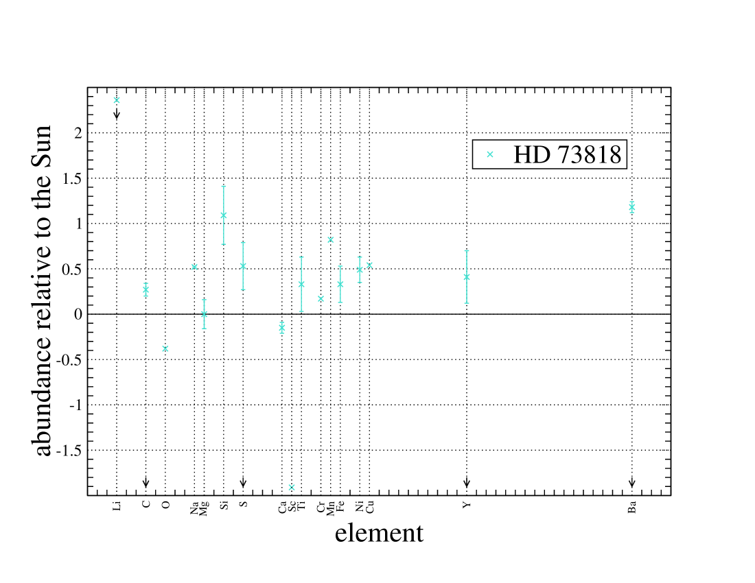
Figure 21: As for Fig. 13 for HD 73818

Table 4: The Table shows the comparison between the abundances described in this paper and those derived by other authors for the common stars. We compare also the fundamental parameters. HBA: Hui-Bon-Hoa et al. (1997); HA: Hui-Bon-Hoa & Alecian (1998); A: Andrievsky (1998); BC: Burkhart & Coupry (1998); TW: This Work.

	$T_{\mathrm{eff}}$	$\log g$	${\upsilon}\sin i$	$\upsilon_{\mathrm{mic}}$	He	Li	C	O	Na	Mg	Al
HD 73666
A	9600	3.80	30	3.0	$-1.05(-)$		$-3.59(-)$	$-3.37(-)$	$-5.41(-)$
BC	9500	$-$	$-$	4.5		$<-8.59(-)$
TW	9382	3.78	10	1.9	$-1.20(05)$	$-$	$<-3.25(03)$	$-3.06(07)$	$-5.47(01)$
HD 72942
HA	8130	3.80	70	2.0						$-4.38(-)$
BC	8300	$-$	$-$	4.5		$<-8.74(-)$
TW	8450	3.90	73	2.4		$<-8.49(-)$				$-4.51(03)$
HD 73045
HBA	7520	4.27	10	3.5						$-4.31(-)$
BC	7500	$-$	$-$	4.5		$-9.04(-)$					$-5.44(-)$
TW	7570	4.05	10	3.6		$-8.86(02)$				$-4.52(04)$	$<-5.41(01)$
HD 73730
HA	8020	3.90	32	4.0						$-4.67(-)$
BC	8020	$-$	$-$	4.5		$-9.04(-)$					$-5.64(-)$
TW	8070	3.97	29	2.6		$-8.74(-)$				$-4.43(06)$	$<-5.37(-)$
HD 73618
HBA	8060	3.87	60	3.0						$-3.93(-)$
A	8050	4.00	60	3.0			$-3.89(-)$	$-3.77(-)$	$-5.71(-)$
BC	8100	$-$	$-$	4.5		$-8.94(-)$					$-5.29(-)$
TW	8170	4.00	47	2.5		$<-8.58(-)$	$<-4.16(16)$	$-3.65(04)$	$-5.34(03)$	$-4.29(-)$	$-$
HD 73174
HA	8090	4.00	$<$10	2.8						$-4.40(-)$
BC	8090	$-$	$-$	4.5		$-9.04(-)$					$-5.34(-)$
TW	8350	4.15	$<$5	2.9		$-8.51(02)$				$-4.21(05)$	$<-5.06(-)$
HD 73711
BC	8290	$-$	$-$	4.5		$<-8.64(-)$
TW	8020	3.69	62	2.5		$<-8.43(-)$
HD 73818
BC	7230	$-$	$-$	4.5		$-8.99(-)$
TW	7230	3.82	66	2.8		$<-8.63(-)$
HD 73709
HBA	8060	3.95	20	3.5						$-4.39(-)$
BC	8080	$-$	$-$	4.5		$-8.64(-)$					$-5.14(-)$
TW	8070	3.78	10	2.3		$-$				$-4.56(06)$	$<-4.91(16)$
	Si	S	Ca	Sc	Cr	Mn	Fe	Ni	Ba	Eu
HD 73666
A	$-4.89(-)$		$-5.68(-)$				$-4.44(-)$		$-9.31(-)$
BC		$-4.64(-)$	$-5.24(-)$				$-3.94(-)$			$-10.04(-)$
TW	$-4.30(01)$	$<-4.47(-)$	$-5.53(14)$				$-4.30(07)$		$<-9.13(04)$	$-$
HD 72942
HA			$-6.09(-)$	$-9.05(-)$	$-6.40(-)$		$-4.59(07)$	$-5.09(-)$
BC		$-4.54(-)$					$-4.29(-)$
TW		$<-4.48(-)$	$-5.58(12)$	$-8.88(11)$	$-6.41(16)$		$-4.47(07)$	$-5.57(-)$
HD 73045
HBA			$-6.22(27)$	$-9.87(-)$	$-5.67(-)$		$-3.95(14)$	$-4.99(-)$
BC	$-4.29(-)$	$-4.94(-)$					$-4.17(-)$	$-5.09(-)$		$-10.54(-)$
TW	$-4.21(05)$	$<-4.67(09)$	$-6.46(04)$	$-9.39(01)$	$-5.63(16)$		$-4.03(04)$	$-4.93(06)$		$-10.20(-)$
HD 73730
HA			$-6.24(-)$	$-10.54(-)$	$-6.06(-)$		$-4.35(06)$	$-5.14(-)$
BC	$-4.39(-)$	$-4.64(-)$					$-4.14(-)$	$-5.34(-)$		$-10.74(-)$
TW	$-4.21(05)$	$<-4.54(03)$	$-6.36(03)$	$-9.71(03)$	$-5.65(08)$		$-4.14(05)$	$-5.14(07)$		$-10.42(-)$
HD 73618
HBA			$-5.70(-)$	$-10.53(-)$	$-5.92(-)$		$-4.08(20)$	$-4.93(-)$
A	$-4.69(-)$	$-4.51(-)$	$-5.78(-)$			$-6.75(-)$	$-4.24(-)$	$-5.49(-)$	$-9.21(-)$
BC	$-4.14(-)$	$-4.74(-)$					$-4.01(-)$
TW	$-4.51(-)$	$<-4.52(13)$	$-5.74(07)$	$-9.51(27)$	$-5.93(10)$	$-6.28(-)$	$-4.13(10)$	$-5.10(15)$	$<-8.09(18)$
HD 73174
HA			$-6.07(07)$	$-10.52(-)$	$-6.09(-)$		$-4.27(16)$	$-5.20(-)$
BC	$-4.34(-)$	$-4.74(-)$					$-4.22(-)$	$-5.24(-)$		$-10.54(-)$
TW	$-4.08(11)$	$<-4.37(03)$	$-5.70(08)$	$-9.44(08)$	$-5.69(08)$		$-3.88(09)$	$-4.79(02)$		$-$
HD 73711
BC		$-4.64(-)$					$-3.94(-)$
TW		$<-4.62(-)$					$-4.44(13)$
HD 73818
BC							$-4.34(-)$
TW							$-4.26(20)$
HD 73709
HBA			$-5.92(17)$	$-10.20(-)$	$-5.72(-)$		$-3.96(17)$	$-4.76(-)$
BC	$-4.24(-)$	$-4.54(-)$					$-4.04(-)$	$-5.04(-)$		$-10.24(-)$
TW	$-4.10(06)$	$<-4.44(01)$	$-6.18(06)$	$-9.79(01)$	$-5.79(13)$		$-4.05(11)$	$-4.88(06)$		$-9.95(-)$