Multi-Orbital Lattice Model for (Ga,Mn)As and Other Lightly Magnetically Doped Zinc-Blende-Type Semiconductors

Abstract

We present a Hamiltonian in real space which is well suited to study numerically the behavior of holes introduced in III-V semiconductors by Mn doping when the III³⁺ ion is replaced by Mn²⁺. We consider the actual lattice with the diamond structure. Since the focus is on light doping by acceptors, a bonding combination of III and V p-orbitals is considered since the top of the valence band, located at the $\Gamma$ point, has p character in these materials. As a result, an effective model in which the holes hop between the sites of an fcc lattice is obtained. We show that around the $\Gamma$ point in momentum space the Hamiltonian for the undoped case is identical to the one for the Luttinger-Kohn model. The spin-orbit interaction is included as well as the on-site interaction between the spin of the magnetic impurity and the spin of the doped holes. The effect of Coulomb interactions between Mn²⁺ and holes, as well as Mn³⁺ doping are discussed. Through large-scale Monte Carlo simulations on a Cray XT3 supercomputer, we show that this model reproduces many experimental results for ${\rm Ga_{\it 1-x}Mn_{\it x}As}$ and ${\rm Ga_{\it 1-x}Mn_{\it x}Sb}$, and that the Curie temperature does not increase monotonically with $x$. The cases of Mn doped GaP and GaN, in which Mn³⁺ is believed to play a role, are also studied.

I Introduction

The discovery of high Curie temperatures ($T_{C}$) in some diluted magnetic semiconductors (DMS)OHN96 ; dietl00 ; Pot has created a renewed interest in the study of the properties of these materials due to their potential role in spintronics devices if above room temperature $T_{C}$’s are achieved.Zutic

When a III-V compound is magnetically doped the added holes can gain kinetic energy by moving in the bands formed by the hybridized orbitals or magnetic energy by interacting with the spin of the localized magnetic impurities. The kinetic term induces delocalization and it is usually studied in momentum space; the magnetic term tends to localize the carriers and it is natural to study it in real space. In the limit of large Mn doping the kinetic term should prevail while in the very diluted regime the magnetic term has to be accurately considered. Most studies of DMS are based in one of these two extreme limits. However, in order to understand the intermediate region between both extremes powerful non-perturbative techniques are needed. The goal of this work is to provide such a tool.

The band structure of Zinc-Blende type semiconductors has been accurately obtained using a variety of different approaches such as pseudopotential methods, tight-binding techniques, and by careful consideration of the symmetries involved through the application of group theory.cardona However, many of these calculations involve a large number of orbitals per site making them unsuitable for simulations of doped systems with present day computers. The successful Luttinger-Kohn model,KL that describes the top of the valence band of semiconductors with diamond structure is very useful to study hole doping in cases of strong hybridization. When the doped holes are not localized they go into the valence band and a formulation of the problem in momentum space is appropriate. This approach, known as the valence band or hole-fluid scenario, has already been applied to DMSmacdonald ; Dietl providing results that would be valid in a regime in which the doped holes are uniformly distributed in the crystal and the randomness in the impurity distribution becomes irrelevant. On the other hand, it is well known that in the limit of strong dilution the doped holes will have a tendency to become localized at the Mn impurities. In this extreme regime holes move by hopping through overlapping orbitals and this behavior is better described in real space. The study of this limit has been carried out only at a phenomenological level using tight binding Hamiltonians that, while taking into account the random position of the impurities, do not provide a realistic band description of the bands resulting from the overlaps of the atomic orbitals involved.Gonz ; Mat ; Ken ; Sarma ; Schl ; Xu

The goal of this paper is to provide a realistic, yet simple, tight-binding-like Hamiltonian, in real space, that reproduces the top of the valence band of Zinc-Blende type semiconductors with the smallest possible number of degrees of freedom per site, and that handles the interactions between the doped holes and the randomly distributed magnetic impurities. It will be shown that six orbitals per site are needed to capture experimental properties of the DMS even in the case of a strong spin-orbit (SO) interaction in which, naively, only four orbitals are relevant at the top of the valence band.cardona This model reproduces the Curie temperatures observed experimentally for various values of Mn doping and compensations and it captures the Curie-Weiss behavior of the magnetization curves in the low compensation regime. It also predicts that for Mn doped GaAs the Curie temperature would pass through a maximum value $T_{C}\approx 220K$ for $x\approx 12\%$ suggesting that higher Mn doping is not the route to achieve room temperature $T_{C}$ with GaAs.

The paper is organized as follows: the general tight binding approach is described in Section II; Section III is devoted to systems in which the spin-orbit interaction can be neglected; the spin-orbit interaction is considered in Section IV by working in a basis formed by total angular momentum eigenstates $|j,m_{j}>$; Section V is devoted to the discussion of Coulomb interactions and how to handle the possibility of Mn³⁺ doping. Numerical results in finite systems for a variety of materials are presented in various subsections of Section VI; conclusions and a summary appear in Section VII. In the Appendix the change of basis matrices are provided.

II Tight Binding approach

Although we will provide a Hamiltonian that can be applied to any III-V semiconductor with Zinc-Blende type structure, we will use Mn doped GaAs as our example. In GaAs, the Ga and As atoms bond covalently. Both atoms share the electrons that they have in their 4s and 4p shells. Ga shares 3 electrons while As shares 5. The hybridized orbitals have character $sp^{3}$. Although the $s$ and $p$ orbitals have to be considered in order to obtain the correct band structure, we are interested in light hole doping for which we will focus only on the valence band, since to facilitate numerical simulations we need to minimize the number of degrees of freedom. It is well known that around the $\Gamma$ point the valence band of GaAs has $j={3\over{2}}$ character, which arises from the original $p$ orbitals.cardona Thus, in order to construct the simplest model that captures this feature we will consider only the $p$ orbitals. The three $p$ orbitals $p_{x}$, $p_{y}$ and $p_{z}$ in each ion can be populated with particles with spin up or down.

To study GaAs we should consider two interpenetrating fcc lattices separated by a distance $(a_{0}/4,a_{0}/4,a_{0}/4)$ were $a_{0}$ is the underlying cubic lattice parameter. The Ga ions seat in one of the fcc lattices and the As ions in the other. Each ion has 4 nearest neighbors of the opposite species located at $(a_{0}/4,a_{0}/4,a_{0}/4)$, $(a_{0}/4,-a_{0}/4,-a_{0}/4)$, $(-a_{0}/4,a_{0}/4,-a_{0}/4)$ and $(-a_{0}/4,-a_{0}/4,a_{0}/4)$.

Since we are only interested in obtaining the valence band we are going to consider the bonding combinations of the Ga and As $p$ orbitals.cardona ; harrison ; chang This leads to an effective fcc lattice with three $p$ bonding orbitals at each site that can be occupied by particles with spin up or down. Thus, working in this $|p,\alpha>$ basis there are 6 states per site of the fcc lattice. We will consider the nearest neighbor hopping of these particles to construct the effective tight-binding Hamiltonian. The twelve nearest neighbors are located at $(\pm a_{0}/2,\pm a_{0}/2,0)$, $(\pm a_{0}/2,0,\pm a_{0}/2)$, $(0,\pm a_{0}/2,\pm a_{0}/2)$ considering the four sign combinations for the three sets of points provided.

In order to calculate the hoppings we follow Slater and Koster.slater The nearest neighbors in our effective fcc lattice are the second nearest neighbors in the original diamond structure. From Table I in Ref.slater, we see that the relevant overlap integrals in this case are

$$E_{xx}=l^{2}(pp\sigma)+(1-l^{2})(pp\pi),$$

$$E_{xy}=lm[(pp\sigma)-(pp\pi)],$$

and

$$E_{xz}=ln[(pp\sigma)-(pp\pi)].$$

The 12 nearest neighbors in the fcc lattice are labeled $(p,q,r)$ following Ref.slater, . For this geometry, two of the indices taking the value $\pm 1$ and the remaining one is 0. Since $l={p\over{\sqrt{p^{2}+q^{2}+r^{2}}}}$ with $(p,q,r)=(1,1,0)$, etc. (we are following Slater’s notation), it follows that $l$, $m$ and $n$ are equal to 0 or $\pm 1/\sqrt{2}$. Then the hoppings to the twelve neighbors that we will label by $(\mu,\nu)$ with $\mu$ and $\nu$ taking the values $\pm x$, $\pm y$,and $\pm z$, are:

$$-t_{\rm aa}^{\mu\nu}=E_{xx}(\mu,\nu)={1\over{2}}[(pp\sigma)+(pp\pi)]=-t_{xx}^{\parallel},$$

if either $\mu={\rm a}$ or $\nu={\rm a}$ or

$$-t_{\rm aa}^{\mu\nu}=E_{xx}(\mu,\nu)=(pp\pi)=-t_{xx}^{\perp},$$

if neither $\nu$ nor $\mu$ are equal to ${\rm a}$, and

$$-t_{\rm ab}^{\mu\nu}=E_{xy}(\mu,\nu)=\pm{1\over{2}}[(pp\sigma)-(pp\pi)]=\mp t_{xy},$$

with the minus (plus) sign for the case in which $\mu$ and $\nu$ have the same (opposite) sign. Also notice that the interorbital hopping is only possible when $(\mu,\nu)$ and ab are in the same plane, i.e., there is no perpendicular interorbital hopping.

III The model without spin-orbit interaction

If the doped Mn ions go into the parent compound as Mn²⁺ replacing Ga³⁺, it means that a hole is doped into the $p$ hybridized orbitals which form the valence band of the undoped semiconductor. This allows us to write a Hamiltonian that takes into account the nearest neighbor hopping of the holes in the $p$ orbitals using the hoppings calculated above, and their magnetic interaction with the localized randomly doped Mn²⁺ ions:

$${\rm H={1\over{2}}\sum_{{\bf i,\mu,\nu},\alpha,a,b}t_{ab}^{\bf\mu\nu}(c^{\dagger}_{{\bf i},\alpha,a}c_{{\bf i+\mu+\nu},\alpha,b}+h.c.)}$$

$$+{\rm J\sum_{{\bf I},a}{\bf s_{I}}^{a}\cdot{\bf S_{I}}},$$

where ${\rm c^{\dagger}_{{\bf i},\alpha,a}}$ creates a hole at site ${\bf i}=({\rm i_{x},i_{y},i_{z}})$ in orbital ${\rm a}$ with spin projection $\alpha$, ${\bf s_{I}}^{\rm a}$=$\rm\sum_{\alpha\beta}c^{\dagger}_{{\bf I},\alpha,a}{\bf{\sigma}}_{\alpha\beta}c_{{\bf I},\beta,a}$ is the spin of the mobile hole, the Pauli matrices are denoted by ${\bf\sigma}$, ${\bf S_{I}}$ is the localized Mn²⁺ spin $5/2$ at site ${\bf I}$ (covering only a small fraction of the total number of sites $N$ since Mn replaces a small number of Ga). $t_{\rm ab}^{\bf\mu\nu}$ are the hopping amplitudes for the holes that were defined in Section II, and ${\rm J>0}$ is an antiferromagnetic (AF) coupling between the spins of the mobile and localized degrees of freedom.oka The density $\rm\langle n\rangle$ of itinerant holes is controlled by a chemical potential. The sites i belong to an fcc lattice and the versors $\bf\mu\nu$ indicate the 12 nearest neighbors of each site i by taking the values $\pm\hat{x}$, $\pm\hat{y}$, and $\pm\hat{z}$, with $\mu\neq\nu$.

Notice that we have only three different hoppings: two intraorbital ones $t_{\rm aa}^{\perp}$ and $t_{\rm aa}^{\parallel}$ and the interorbital ones $t_{\rm ab}$. All have the same absolute value (but not always the same sign) for all combination of orbitals and neighbors. The interorbital hoppings that have the sign reversed are the ones towards sites labeled by $\mu$ and $\nu$ with opposite signs, i.e. $-t_{\rm xx}^{x,y}=t_{\rm xx}^{-x,y}$. Also notice that the interorbital hoppings occur only in the planes defined by the two orbitals, i.e., they vanish in the direction perpendicular to the plane were the two orbitals are $t_{\rm xz}^{x,y}=0$. This can be seen in the expressions provided in Eq.(1).

In order to obtain the material specific values of the hopping parameters we will write the Hamiltonian matrix in momentum space for the undoped case, i.e., Eq.(3) with $J=0$. We can use Table II or III in Ref.slater, to do this task. The result is given by,

$$T=\left(\begin{array}[]{ccc}T_{x}&-t_{xy}s_{xy}&-t_{xy}s_{xz}\\ -t_{xy}s_{xy}&T_{y}&-t_{xy}s_{yz}\\ -t_{xy}s_{xz}&-t_{xy}s_{yz}&T_{z}\end{array}\right),$$

for spin up and an identical block for spin down. Here $T_{x}=4t_{xx}^{\parallel}(c_{x}c_{y}+c_{x}c_{z})+4t_{xx}^{\perp}c_{y}c_{z}$, $T_{y}=4t_{xx}^{\parallel}(c_{x}c_{y}+c_{y}c_{z})+4t_{xx}^{\perp}c_{x}c_{z}$, $T_{z}=4t_{xx}^{\parallel}(c_{x}c_{z}+c_{y}c_{z})+4t_{xx}^{\perp}c_{x}c_{y}$, and $s_{ij}=4s_{i}s_{j}$ with $c_{i}={\rm cos}(ak_{i})$, $s_{i}={\rm sin}(ak_{i})$, where in Slater’s notation $a=a_{0}/2$, with $a_{0}$ the Zinc-Blende lattice constant and $k_{i}$ are the momentum components along $i=x,y$, or $z$.

We mentioned in the introduction that Luttinger and Kohn studied the movement of holes in the valence band of semiconductors with the diamond structure. Working in momentum space they found an expression for the Hamiltonian matrix that describes the top of the valence band, i.e., the neighborhood of the $\Gamma$ point. In the $|p,\alpha>$ basis the matrix has the form:

$$\left(\begin{array}[]{ccc}Ak_{x}^{2}+B(k_{y}^{2}+k_{z}^{2})&Ck_{x}k_{y}&Ck_{x}k_{z}\\ Ck_{x}k_{y}&Ak_{y}^{2}+B(k_{x}^{2}+k_{z}^{2})&Ck_{y}k_{z}\\ Ck_{x}k_{z}&Ck_{y}k_{z}&Ak_{z}^{2}+B(k_{x}^{2}+k_{y}^{2})\end{array}\right).$$

There is an identical block for spin down. $A$, $B$ and $C$ are constants that can be defined in terms of the Luttinger parameters $\gamma_{1}$, $\gamma_{2}$, and $\gamma_{3}$(Lut, ) which are material specific. The accepted values for GaAs are $(\gamma_{1},\gamma_{2},\gamma_{3})=(6.85,2.1,2.9)$.cardona ; macdonald The constants are given by:

$$A=-{\hbar^{2}\over{2m}}(\gamma_{1}+4\gamma_{2}),$$

$$B=-{\hbar^{2}\over{2m}}(\gamma_{1}-2\gamma_{2}),$$

$$C=-6{\hbar^{2}\over{2m}}\gamma_{3},$$

where $m$ is the mass of the bare electron.

Remembering that Eq.(5) is an approximation valid for the top of the valence band (i.e. the $\Gamma$ point), we can expand the cosines and sines in Eq.(4) and we obtain the matrix shown in Eq.(5) if we disregard a constant term along the diagonal that just shifts the top of the valence band to $8t_{xx}^{\parallel}+4t_{xx}^{\perp}$ instead of 0. Comparing the coefficients we obtain expressions for the hoppings in terms of the Luttinger parameters and the lattice constant $a_{0}=2a$:chang1

$$t_{xx}^{\parallel}={\hbar^{2}\over{8ma^{2}}}(\gamma_{1}+4\gamma_{2})={\hbar^{2}\over{2ma_{0}^{2}}}(\gamma_{1}+4\gamma_{2}),$$

$$t_{xx}^{\perp}={\hbar^{2}\over{8ma^{2}}}(\gamma_{1}-8\gamma_{2})={\hbar^{2}\over{2ma_{0}^{2}}}(\gamma_{1}-8\gamma_{2}),$$

$$t_{xy}={3\hbar^{2}\over{4ma^{2}}}\gamma_{3}={3\hbar^{2}\over{ma_{0}^{2}}}\gamma_{3}.$$

Since our goal is to write a tight-binding Hamiltonian for holes that will dope at most the bottom of the band, we will reverse the signs of the hoppings since the band obtained in Eq.(5) gets reflected with respect to zero by reversing the signs of $A$, $B$, and $C$.foot Then, for GaAs, $a_{0}=5.64\AA$, cardona and from Eq.(7) we obtain:

$$t_{xx}^{\parallel}=-1.82eV,\quad t_{xx}^{\perp}=1.20eV,\quad t_{xy}=-2.08eV.$$

It is important to notice that the evaluation of the hopping parameters given by Eq.(7) requires three independent parameters to fix their values. However, if we look at the expression for the hoppings given in Eq.(2) in terms of overlap integrals it would appear incorrectly as if only two parameters were necessary and the three hoppings should be interrelated. The evaluation Eq.(7) is more accurate though because it considers, in a phenomenological way, the influence of the neglected bands in the shape of the valence band at $\Gamma$.

IV Spin-Orbit interaction

The spin-orbit interaction is important in GaAs and in other III-V semiconductors in which the ion V has a large mass. It mixes the angular momentum ($l=1$ for the $p$ orbitals) with the holes’ spin degrees of freedom producing states with $j={3\over{2}}$ and $j={1\over{2}}$. In a cubic lattice with the diamond symmetry, Luttinger and Kohn showed that at the $\Gamma$ point the states with $j={1\over{2}}$ get separated from those with $j={3\over{2}}$ which are the relevant states at the top of the valence band. As a result, naively only four states per site, instead of six, become relevant when the spin-orbit interaction is considered and the doping is light.KL However, as it will be shown in Section VI, at the levels of doping of interest ($x\geq 3$%) the heavy and light hole states that become populated are sufficiently separated from the $\Gamma$ point that the $j=1/2$ contribution becomes important.

To take into account the spin-orbit interaction we will have to perform a change of basis from $|p,\alpha>$ to $|j,m_{j}>$. This change of basis has been studied by Kohn and Luttinger.KL

The Luttinger-Kohn matrix (Eq.5) in the $|j,m_{j}>$ basis is presented in Eq.(A8) of Ref.macdonald, .

The six states that form the basis are:

$$|1>=|{3\over{2}},{3\over{2}}>,\quad|2>=|{3\over{2}},-{1\over{2}}>,\quad|3>=|{3\over{2}},{1\over{2}}>,$$

$$|4>=|{3\over{2}},-{3\over{2}}>,\quad|5>=|{1\over{2}},{1\over{2}}>,\quad|6>=|{1\over{2}},-{1\over{2}}>.$$

Applying the same change of basis to $U=\left(\begin{array}[]{cc}T&0\\ 0&T\end{array}\right)$ with $T$ given in Eq.(4) we obtain the $6\times 6$ matrix $U^{\prime}=MUM^{-1}$ where $M$ is the change of basis matrix provided in Appendix I.

$$U^{\prime}=\left(\begin{array}[]{cccccc}H_{hh}&-c&-b&0&{b\over{\sqrt{2}}}&c\sqrt{2}\\ -c^{*}&H_{lh}&0&b&-b^{*}\sqrt{3\over{2}}&-d\\ -b^{*}&0&H_{lh}&-c&d&-b\sqrt{3\over{2}}\\ 0&b^{*}&-c^{*}&H_{hh}&-c^{*}\sqrt{2}&{b^{*}\over{\sqrt{2}}}\\ {b^{*}\over{\sqrt{2}}}&-b\sqrt{3\over{2}}&d^{*}&-c\sqrt{2}&H_{so}&0\\ c^{*}\sqrt{2}&-d^{*}&-b^{*}\sqrt{3\over{2}}&{b\over{\sqrt{2}}}&0&H_{so}\end{array}\right),$$

with

$$H_{hh}=4t_{x,x}^{\parallel}c_{x}c_{y}+2(t_{x,x}^{\perp}+t_{x,x}^{\parallel})(c_{x}c_{z}+c_{y}c_{z}),$$

$$H_{lh}={2\over{3}}(5t_{x,x}^{\parallel}+t_{x,x}^{\perp})(c_{y}c_{z}+c_{x}c_{z})+{4\over{3}}(t_{x,x}^{\parallel}+2t_{x,x}^{\perp})c_{x}c_{y},$$

$$b={-4\over{\sqrt{3}}}t_{x,y}(s_{x}s_{z}+is_{y}s_{z}),$$

$$c={2\over{\sqrt{3}}}(t_{x,x}^{\parallel}-t_{x,x}^{\perp})(c_{x}c_{z}-c_{y}c_{z})-{4i\over{\sqrt{3}}}t_{x,y}s_{x}s_{y},$$

$$d=4({\sqrt{2}\over{3}}(t_{x,x}^{\parallel}-t_{x,x}^{\perp})c_{x}c_{y}-{(t_{x,x}^{\parallel}-t_{x,x}^{\perp})\over{3\sqrt{2}}}(c_{x}c_{z}+c_{y}c_{z})),$$

$$H_{so}=4{(2t_{x,x}^{\parallel}+t_{x,x}^{\perp})\over{3}}(c_{x}c_{y}+c_{x}c_{z}+c_{y}c_{z})+\Delta_{SO},$$

where $\Delta_{SO}$ is the spin-orbit splitting which is tabulated for different materials.cardona The matrix in Eq.(10) agrees with Eq.A8 in Ref.macdonald, in the limit of small $k$.

IV.1 Hoppings between $|j,m_{j}>$ States in Real Space

Now we need to calculate the hoppings in real space between the 6 orbitals characterized by $j={3\over{2}}$ and $m_{j}=\pm{3\over{2}}$ and $\pm{1\over{2}}$ and $j={1\over{2}}$ with $m_{j}=\pm{\tilde{1}\over{2}}$.

To do this, we need to express the $c$ operators that appear in Eq.(3) in terms of the $c$ operators in the basis $|j,m_{j}>$ with the help of the basis transformation given in the Appendix:

$$\left(\begin{array}[]{cccccc}c^{\dagger}_{{\bf i},{3\over{2}},{3\over{2}}}&c^{\dagger}_{{\bf i},{3\over{2}},-{1\over{2}}}&c^{\dagger}_{{\bf i},{3\over{2}},{1\over{2}}}&c^{\dagger}_{{\bf i},{3\over{2}},-{3\over{2}}}&c^{\dagger}_{{\bf i},{1\over{2}},{1\over{2}}}&c^{\dagger}_{{\bf i},{1\over{2}},-{1\over{2}}}\end{array}\right)M=\left(\begin{array}[]{cccccc}c^{\dagger}_{{\bf i},\uparrow,x}&c^{\dagger}_{{\bf i},\uparrow,y}&c^{\dagger}_{{\bf i},\uparrow,z}&c^{\dagger}_{{\bf i},\downarrow,x}&c^{\dagger}_{{\bf i},\downarrow,y}&c^{\dagger}_{{\bf i},\downarrow,z}\end{array}\right)$$

and

$$M^{-1}\left(\begin{array}[]{c}c_{{\bf i},{3\over{2}},{3\over{2}}}\\ c_{{\bf i},{3\over{2}},-{1\over{2}}}\\ c_{{\bf i},{3\over{2}},{1\over{2}}}\\ c_{{\bf i},{3\over{2}},-{3\over{2}}}\\ c_{{\bf i},{1\over{2}},{1\over{2}}}\\ c_{{\bf i},{1\over{2}},-{1\over{2}}}\end{array}\right)=\left(\begin{array}[]{c}c_{{\bf i},\uparrow,x}\\ c_{{\bf i},\uparrow,y}\\ c_{{\bf i},\uparrow,z}\\ c_{{\bf i},\downarrow,x}\\ c_{{\bf i},\downarrow,y}\\ c_{{\bf i},\downarrow,z}\end{array}\right).$$

We obtain:

$$c^{\dagger}_{{\bf i},\sigma,x}=\sigma({-1\over{\sqrt{2}}}c^{\dagger}_{{\bf i},{3\over{2}},\sigma{3\over{2}}}+{1\over{\sqrt{6}}}c^{\dagger}_{{\bf i},{3\over{2}},-\sigma{1\over{2}}})-{1\over{\sqrt{3}}}c^{\dagger}_{{\bf i},{1\over{2}},-\sigma{1\over{2}}},$$

$$c^{\dagger}_{{\bf i},\sigma,y}=-i({1\over{\sqrt{2}}}c^{\dagger}_{{\bf i},{3\over{2}},\sigma{3\over{2}}}+{1\over{\sqrt{6}}}c^{\dagger}_{{\bf i},{3\over{2}},-\sigma{1\over{2}}}-{\sigma\over{\sqrt{3}}}c^{\dagger}_{{\bf i},{1\over{2}},-\sigma{1\over{2}}}),$$

$$c^{\dagger}_{{\bf i},\sigma,z}=\sqrt{{2\over{3}}}c^{\dagger}_{{\bf i},{3\over{2}},\sigma{1\over{2}}}-\sigma\sqrt{{1\over{3}}}c^{\dagger}_{{\bf i},{1\over{2}},\sigma{1\over{2}}},$$

and

$$c_{{\bf i},\sigma,x}=\sigma({-1\over{\sqrt{2}}}c_{{\bf i},{3\over{2}},\sigma{3\over{2}}}+{1\over{\sqrt{6}}}c_{{\bf i},{3\over{2}},-\sigma{1\over{2}}})-{1\over{\sqrt{3}}}c_{{\bf i},{1\over{2}},-\sigma{1\over{2}}},$$

$$c_{{\bf i},\sigma,y}=i({1\over{\sqrt{2}}}c_{{\bf i},{3\over{2}},\sigma{3\over{2}}}+{1\over{\sqrt{6}}}c_{{\bf i},{3\over{2}},-\sigma{1\over{2}}})-{i\sigma\over{\sqrt{3}}}c_{{\bf i},{1\over{2}},-\sigma{1\over{2}}},$$

$$c_{{\bf i},\sigma,z}=\sqrt{{2\over{3}}}c_{{\bf i},{3\over{2}},\sigma{1\over{2}}}-\sigma{1\over{\sqrt{3}}}c_{{\bf i},{1\over{2}},\sigma{1\over{2}}}.$$

Replacing in Eq.(3) and rearranging the terms we find that the intraorbital hoppings are given by:

$$t^{x,y}_{\sigma{3\over{2}},\sigma{3\over{2}}}=t_{xx}^{\parallel},\quad t^{x,y}_{\sigma{1\over{2}},\sigma{1\over{2}}}={t_{xx}^{\parallel}+2t_{xx}^{\perp}\over{3}}$$

$$t^{y,z}_{\sigma{3\over{2}},\sigma{3\over{2}}}=t^{x,z}_{\sigma{3\over{2}},\sigma{3\over{2}}}={(t_{xx}^{\parallel}+t_{xx}^{\perp})\over{2}}$$

$$t^{y,z}_{\sigma{1\over{2}},\sigma{1\over{2}}}=t^{x,z}_{\sigma{1\over{2}},\sigma{1\over{2}}}={(5t_{xx}^{\parallel}+t_{xx}^{\perp})\over{6}}$$

$$t^{\mu,\nu}_{\sigma{\tilde{1}\over{2}},\sigma{\tilde{1}\over{2}}}={2t_{xx}^{\parallel}+t_{xx}^{\perp}\over{3}}$$

Now let us consider the inter-orbital hoppings between orbitals with $j=3/2$:

$$t^{x,z}_{\rm\sigma a,-\sigma a^{\prime}}=-t^{y,z}_{\rm\sigma a,-\sigma a^{\prime}}={(t_{xx}^{\perp}-t_{xx}^{\parallel})\over{\sqrt{12}}},$$

$$t^{x,y}_{\rm a,-a^{\prime}}=(t^{x,y}_{\rm a,-a^{\prime}})^{*}=t^{y,z}_{\sigma 1/2,\sigma 3/2}=(t^{y,z}_{\sigma 3/2,\sigma 1/2})^{*}={i\over{\sqrt{3}}}t_{xy}^{\mu,\nu}$$

$$t^{x,z}_{\rm\sigma a,\sigma a^{\prime}}=\sigma{t_{xy}^{\mu,\nu}\over{\sqrt{3}}},\quad t^{x,y}_{\rm\sigma a,\sigma a^{\prime}}=0.$$

and

$$t^{\mu,\nu}_{\rm\sigma a,-\sigma a}=0,$$

where ${\rm a\neq a^{\prime}}$ in the above expressions.

There are no interorbital hoppings between the two $j=1/2$ orbitals, i.e,

$$t^{\mu,\nu}_{\rm\sigma a,-\sigma a}=0,$$

if $a={\tilde{1}\over{2}}$, i.e., the symbol that we use to represent $m_{j}$ for the orbitals with $j={1\over{2}}$.

The interorbital hoppings between $j=3/2$ and $j=1/2$ orbitals are given by:

$$t^{xz}_{\rm\sigma{\tilde{1}\over{2}},\sigma{3\over{2}}}=t^{xz}_{\rm\sigma{3\over{2}},\sigma{\tilde{1}\over{2}}}=-{t_{xy}^{\mu,\nu}\over{\sqrt{6}}}$$

$$t^{yz}_{\rm\sigma{3\over{2}},\sigma{\tilde{1}\over{2}}}=(t^{yz}_{\rm\sigma{\tilde{1}\over{2}},\sigma{3\over{2}}})^{*}=-i{t_{xy}^{\mu,\nu}\over{\sqrt{6}}}$$

$$t^{xz}_{\rm\sigma{1\over{2}},-\sigma{\tilde{1}\over{2}}}=t^{xz}_{\rm\sigma{\tilde{1}\over{2}},-\sigma{1\over{2}}}={t_{xy}^{\mu,\nu}\over{\sqrt{2}}}$$

$$t^{yz}_{\rm\sigma{1\over{2}},-\sigma{\tilde{1}\over{2}}}=t^{yz}_{\rm\sigma{\tilde{1}\over{2}},-\sigma{1\over{2}}}=i\sigma{t_{xy}^{\mu,\nu}\over{\sqrt{2}}}.$$

$$t^{x,y}_{\rm\sigma{1\over{2}},\sigma{\tilde{1}\over{2}}}=t^{x,y}_{\rm\sigma{\tilde{1}\over{2}},\sigma{1\over{2}}}=-\sigma{\sqrt{2}(t_{xx}^{\perp}-t_{xx}^{\parallel})\over{3}},$$

$$t^{x,z}_{\rm\sigma{1\over{2}},\sigma{\tilde{1}\over{2}}}=t^{y,z}_{\rm\sigma{1\over{2}},\sigma{\tilde{1}\over{2}}}=t^{x,z}_{\rm\sigma{\tilde{1}\over{2}},\sigma{1\over{2}}}=t^{y,z}_{\rm\sigma{\tilde{1}\over{2}},\sigma{1\over{2}}}=\sigma{(t_{xx}^{\perp}-t_{xx}^{\parallel})\over{3\sqrt{2}}},$$

The actual numerical values are obtained using Eq.(7). chang2 Notice that the hoppings can also be read from the matrix elements in Eq.(10).

IV.2 Hund Coupling and the Classical Limit of the Localized Spin

The Hund term in Eq.(3) has the form

$$H_{\bf I}=J{\bf S_{I}\cdot s_{I}},$$

where ${\bf S_{I}}$ is a dimensionless quantum spin 5/2 operator, spin ; Linnar ${\bf s_{I}}$ is a dimensionless quantum spin 1/2 operator, and $J$, which has units of energy (eV), is determined experimentally.oka ; matsu ; macdonald

In order to perform numerical calculations avoiding the sign problemsign which arises when four-fermion interactions, such as in Eq.(16), are decoupled, we are going to take the classical limit for the localized spins. This is a good approximation given the large value, 5/2, of this spin. The classical limit is given by $\hbar\rightarrow 0$, $S\rightarrow\infty$. In order to take the limit correctly Eq.(16) is rewritten as

$$H_{\bf I}=J[S(S+1)]^{1/2}{\cal S}_{\bf I}\cdot{\bf s_{I}},$$

where ${\cal S}_{\bf I}$ is a unit spin quantum operator.

It is important to realize that the Hund coupling $J$ is proportional to $\hbar$ since the spin operators in Eq.(16) are dimensionless. This means that $\lim_{\hbar\to 0}J=0$. However, $\lim_{\hbar\to 0,S\to\infty}J[S(S+1)]^{1/2}=\lim_{\hbar\to 0,S\to\infty}JS$, should be finite. Defining

$$\lim_{\hbar\to 0,S\to\infty}JS=J_{c},$$

in the classical limit Eq.(17) becomes

$$H_{\bf I}=J_{c}{\cal S}_{\bf I}\cdot{\bf s_{I}},$$

where now

$${\cal S}_{\bf I}=({\rm sin\theta_{\bf i}cos\phi_{\bf i},sin\theta_{\bf i}sin\phi_{\bf i},cos\theta_{\bf i}}),$$

is a classical unit vector. ${\bf s_{I}}$ is still a quantum spin-1/2 operator and $J_{c}$ is a parameter. The value of $J_{c}$ should be determined by comparing numerical results to experimental data. For Mn doped GaAs comparing numerical values of the Curie temperature to experimental data, we have observed we that $J_{c}\approx J$. This indicates that

$$\lim_{\hbar\to 0,S\to\infty}JS=J,$$

which is equivalent to

$$\lim_{\hbar\to 0,S\to\infty}\hbar S=\hbar_{0}=6.58\times 10^{-16}eV,$$

i.e., the classical limit according to Ref.classical, .

Additional support for these results is obtained measuring the splitting of the 4 degenerate states at the top of the valence band as a function of $J$. Experimentalists use this split to determine $J$.spin ; Linnar ; Szc According to mean-field calculations the splitted levels have energy $\pm B_{G}$ and $\pm 3B_{G}$ withFurd ; Dietl ; Szc

$$B_{G}={1\over{6}}JxS,$$

with $S=5/2$.spin ; Linnar According to Eq.(23)

$$B_{G}^{c}=\lim_{\hbar\to 0,S\to\infty}B_{G}={1\over{6}}J_{c}x\equiv{1\over{6}}Jx.$$

Our numerical results indicate that the split of the top of the valence band depends linearly on $J$ for values up to $J\leq 0.5$ eV (see subsection VI.C). In Fig.1 we show the mean field value of $B_{G}$, i.e., $B_{G}^{MF}$, calculated using Eq.(23) as a function of $J$ for $x=0.085$ and $x=0.05$ indicated with doted lines. We also display the extrapolated linear behavior obtained numerically for $J\leq 0.5$ eV and the same values of $x$ at $T\to 0$ with our Hamiltonian. The curves indicating $B_{G}^{C}$ in the figure have been obtained by monitoring the energy of the four lowest eigenvalues of Eq.(31) as a function of $J$. In the linear regime we observe that the ratio between $B_{G}^{MF}$ given by Eq.(23) and the measured numerical value in the classical approximation $B_{G}^{C}$ is equal to $S=2.5$ as expected. The excellent numerical agreement between $B_{G}^{MF}/S$ and $B_{G}^{c}$ supporting the result of Eq.(24) is clear in Fig.1.

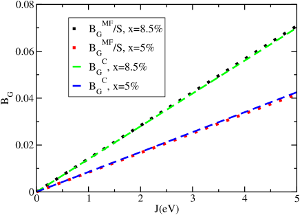
Figure 1: (color online) $B_{G}^{MF}/S$ vs $J$ for $x=0.085$ and 0.05 obtained using Eq.(23) (doted lines) and $B_{G}^{c}$ vs $J$ calculated numerically (extrapolating from the linear regime) with our model for the same values of $x$ (dashed lines).

Now let us consider the Hund coupling term in Eq.(3) in the $|j,m_{j}>$ basis. Eq.(A.10) in Ref.macdonald, has expressions for the spin operators in the $|j,m_{j}>$ basis:

$$s_{x}=\left(\begin{array}[]{cccccc}0&0&{1\over{2\sqrt{3}}}&0&{1\over{\sqrt{6}}}&0\\ 0&0&{1\over{3}}&{1\over{2\sqrt{3}}}&-{1\over{3\sqrt{2}}}&0\\ {1\over{2\sqrt{3}}}&{1\over{3}}&0&0&0&{1\over{3\sqrt{2}}}\\ 0&{1\over{2\sqrt{3}}}&0&0&0&-{1\over{\sqrt{6}}}\\ {1\over{\sqrt{6}}}&-{1\over{3\sqrt{2}}}&0&0&0&-{1\over{6}}\\ 0&0&{1\over{3\sqrt{2}}}&-{1\over{\sqrt{6}}}&{-1\over{6}}&0\end{array}\right)$$

$$s_{y}=i\left(\begin{array}[]{cccccc}0&0&{-1\over{2\sqrt{3}}}&0&-{1\over{\sqrt{6}}}&0\\ 0&0&{1\over{3}}&{-1\over{2\sqrt{3}}}&-{1\over{3\sqrt{2}}}&0\\ {1\over{2\sqrt{3}}}&{-1\over{3}}&0&0&0&-{1\over{3\sqrt{2}}}\\ 0&{1\over{2\sqrt{3}}}&0&0&0&-{1\over{\sqrt{6}}}\\ {1\over{\sqrt{6}}}&{1\over{3\sqrt{2}}}&0&0&0&{1\over{6}}\\ 0&0&{1\over{3\sqrt{2}}}&{1\over{\sqrt{6}}}&-{1\over{6}}&0\end{array}\right)$$

$$s_{z}=\left(\begin{array}[]{cccccc}{1\over{2}}&0&0&0&0&0\\ 0&{-1\over{6}}&0&0&0&-{\sqrt{2}\over{3}}\\ 0&0&{1\over{6}}&0&-{\sqrt{2}\over{3}}&0\\ 0&0&0&{-1\over{2}}&0&0\\ 0&0&-{\sqrt{2}\over{3}}&0&-{1\over{6}}&0\\ 0&-{\sqrt{2}\over{3}}&0&0&0&{1\over{6}}\end{array}\right)$$

Then

$$J{\bf S_{I}\cdot s_{I}}\rightarrow J(S_{\bf I}^{x}s_{\bf I}^{x}+S_{\bf I}^{y}s_{\bf I}^{y}+S_{\bf I}^{z}s_{\bf I}^{z})$$

where

$$s_{\bf I}^{\alpha}={\bf c_{I}}^{\dagger}s_{\alpha}{\bf c_{I}}$$

with

$${\bf c_{I}}^{\dagger}=\left(\begin{array}[]{cccccc}c^{\dagger}_{{\bf i},{3\over{2}}}&c^{\dagger}_{{\bf i},-{1\over{2}}}&c^{\dagger}_{{\bf i},{1\over{2}}}&c^{\dagger}_{{\bf i},-{3\over{2}}}&c^{\dagger}_{{\bf i},{\tilde{1}\over{2}}}&c^{\dagger}_{{\bf i},-{\tilde{1}\over{2}}}\end{array}\right)$$

and under the classical approximation that we just discussed,

$$S_{\bf I}^{x}={\rm sin\theta_{\bf i}cos\phi_{\bf i}},\quad S_{\bf I}^{y}={\rm sin\theta_{\bf i}sin\phi_{\bf i}},\quad S_{\bf I}^{z}={\rm cos\theta_{\bf i}}.$$

Notice that the Mn ions replace Ga so they will be present in a subset of the points of the fcc lattice that we are considering. The values of $J$ can be obtained from comparing experimental data with theoretical models and are material dependent. In the notation of Ref.Dietl, , $J$ in Eq.(26) is given by $\beta N_{0}$ where $\beta$ has units of $eVnm^{3}$ and $N_{0}$ is the concentration of cation sites given by $4a_{0}^{-3}$ where $a_{0}$ is the lattice parameter of the material. $\beta$ is assumed to depend only on the characteristics of the parent material and it is considered the same for all III-V semiconductors. Notice that $\beta$ is called $J_{pd}$ by some authors.macdonald Ref.Dietl, estimates $J$ for GaN and other materials assuming that the accepted value for GaAs is accurate and given by $J=4\beta a_{0}^{-3}=-1.2eV$.oka However, in the literature the value of $J$ for GaAs ranges between $-0.89eV\geq J\geq-3.34eV$.oka ; matsu ; macdonald Using the parameters for GaAs we can estimate that $-0.04eVnm^{3}\geq\beta_{III-V}\geq-0.15eVnm^{3}$.

Then, $J$ for a general III-V material $M$ is given by

$$J_{M}={4\beta_{III-V}\over{a_{0_{M}}^{3}}}.$$

The sign depends on the definition. It seems to be antiferromagnetic for GaAs which means that we need to take it as a positive number in our Hamiltonian. The sign of $J$ is still under discussion for some of the III-V compounds such as GaN.GaNsign However, under the classical spin approximation discussed above, the sign of $J$ in the Hamiltonian becomes irrelevant since the eigenvalues of $H$ are the same for both signs.

Notice that using the parameters provided in this paper, numerical calculations of the critical temperature will be obtained directly in eV.

IV.3 Six-Orbital Real-Space Hamiltonian

Combining the results in the previous subsections the Hamiltonian in the $|j,m_{j}>$ basis can be written as:

$${\rm H={1\over{2}}\sum_{{\bf i,\mu,\nu},\alpha,\alpha^{\prime},a,b}(t_{\alpha a,\alpha^{\prime}b}^{\bf\mu\nu}c^{\dagger}_{{\bf i},\alpha a}c_{{\bf i+\mu+\nu},\alpha^{\prime}b}+h.c.)}$$

$$+\Delta_{SO}\sum_{{\bf i},\alpha}c^{\dagger}_{{\bf i},\alpha{\tilde{1}\over{2}}}c_{{\bf i},\alpha{\tilde{1}\over{2}}}+{\rm J\sum_{{\bf I}}{\bf s_{I}}\cdot{\bf S_{I}}},$$

where ${\rm a,b}$ take the values ${1\over{2}}$, ${\tilde{1}\over{2}}$ or ${3\over{2}}$, $\alpha$ and $\alpha^{\prime}$ can be $1$ or $-1$, and the Hund term is given by Eq.(26). Notice that $\bf\mu+\nu$ are the twelve vectors indicating the twelve nearest neighbor sites of each ion at site i and that I are random sites in the fcc lattice. To reproduce the correct physics we will have to work with an almost filled valence band, i.e., a very low density of holes. Eq.(31) is the Hamiltonian that has to be programmed in the computer simulations. Since there are six states per site, a $6N_{s}\times 6N_{s}$ matrix needs to be diagonalized at each step of a Monte Carlo (MC) simulation; $N_{s}$ is the number of sites in the fcc lattice.

The material dependent hopping parameters are given by Eq.(7) and (15), and the Hund coupling by Eq.(30) (or from experiments if available). $\Delta_{SO}$ is given by the magnitude of the gap between the top of the valence band and the split-off band induced by the spin-orbit interaction. Its value is 0.341eV for GaAs, 0.75eV for GaSb, and 0.017eV for GaN.cardona Thus, it is clear that all the parameters in the proposed Hamiltonian are fixed, i.e., there are no free parameters.

V Additional Effects of the doped Mn Ions

In this section we will consider, at a phenomenological level, the effects of Mn doping that go beyond the mere introduction of a localized spin at the doping site $I$ and the addition of holes into the system.

Up to this point we have implicitly assumed that the Mn $d$ levels are deep into the valence band of the parent compound so that when a Mn ion replaces Ga in GaAs, Ga³⁺ is replaced by Mn²⁺ and a hole is introduced in the $p$ orbitals. In this case, negative charge with respect to the background at the Mn site creates an attractive Coulomb potential for the hole which, in the case of one single Mn ion, contributes to producing a bound state at 0.1eV above the top of the valence band.matsu ; Linnar This bound state is expected to generate an impurity band at least for very light amounts of doping. This impurity band, due to hybridization, eventually will merge with the valence band as the amount of doping increases. For GaAs it is believed that the merging occurs for $x<0.01$Fleurov ; Popescu and for this reason the Coulomb interaction is not expected to play a role in the relevant doping regime. However, the explicit addition of a Coulomb term to the Hamiltonian is important in order to reproduce the GaAs behavior at very low dopings and, in materials for which the hole binding energy is larger, such as GaP and GaN.Koro ; Kreis Thus, below, in subsection A, we are going to describe how to introduce Coulomb attraction in our model.

Another effect that is in general ignored in studies of (Ga,Mn)As is the presence of Mn³⁺ ions. While experiments appear to indicate that Ga³⁺ is replaced by Mn²⁺ in GaAs,Schneider ; spin Mn³⁺ has been reported in GaPKreis and GaN.Kro ; Graf Thus, in order to extend the present model to other materials, in subsection B we will describe a phenomenological way of considering the Mn $d$ orbitals.

V.1 Coulomb Potential

The Coulomb potential between the localized impurities and the doped holes is neglected in most models for DMSGonz ; Mat ; Ken ; Sarma ; Schl ; Xu since the magnetic interaction appears to be sufficient to capture qualitatively many properties of these materials including ferromagnetism, and because it is believed that at the levels of doping for which the material is metallic it will not play a relevant role.Fleurov ; Popescu However, these assumptions need to be confirmed by actual calculations. Very few attempts to include the Coulomb interaction studying its effects with unbiased approaches have been carried out. The case of a single Mn impurity in GaAs was studied in Ref.guill, . They considered the long range Coulomb potential suplemented by a central cell correction with a square-well shape that is routinely applied in calculations of bound state energies for impurities in semiconductors.pante This is the portion of the potential that is expected to be relevant at higher doping since the long-range part will be screened. This effect has been incorporated by many authorstaka ; calde ; hwang ; Popescu by considering an on-site central-cell potential of the form:

$$H_{C}=-V\sum_{I}n_{I}.$$

The value of $V$ varies widely in the literature. Many authors determine it by finding the value that added to $J$ reproduces the energy of the single hole bound state.guill ; taka ; Popescu However, the value of $V$ depends strongly on the characteristic of the model used such as the total bandwidth, the number of orbitals, etc. In other investigations $V$ is considered a free parameter that can even take negative values, i.e., repulsive rather than attractive according to the notation of Eq.(32).calde ; hwang Repulsive potentials are sometimes introduced to reproduce apparent $x$ dependences of the magnetic coupling $J$ observed in some experiments on Mn doped GaNDIETL07 and CdS.TWOR94

However, it was pointed out in Ref.Popescu, that an on-site range potential prevents the overlap of localized hole-wave functions that should occur with increasing doping. It was proposed that a nearest-neighbor range potential should be used, and MC calculations performed on a highly doped single orbital model showed that an impurity band generated by the on-site potential vanished when a nearest-neighbor range potential of the same strength was used. In the fcc lattice considered here, the extended potential has the form

$$H_{C}^{nn}=-V\sum_{I}({1\over{N_{I}}}n_{I}+\sum_{\mu,\nu}{1\over{N_{I+\mu+\nu}}}n_{I+\mu+\nu}),$$

where $V$ is added at the site I in which the impurity is located and at its 12 nearest neighbors I+$\mu+\nu$. $N_{I}$ indicates the number of impurity sites that surround the impurity site $I$. Calculations using both Eq.(32) and (33) will be presented in Section VI.E.

V.2 Mn³⁺

The phenomenology described in the previous subsection is expected to occur when the Mn $d$ orbitals lie deep into the valence band so that Mn²⁺ replaces the III³⁺ ion and the doped hole goes into the $p$ orbitals. However, if the Mn $d$ levels were in the parent compound’s gap, the III³⁺ ion could be replaced by Mn³⁺ with the hole in its $3d$ shell. The $3d$ shell of Mn is splitted into three $t_{2g}$ states and two $e_{g}$ states due to the crystal field. It is believed that the hole goes into the $t_{2g}$ levels.hole Although no Mn³⁺ has been observed in GaAs, there are some indications of it in GaP and GaN.Kreis ; Kro ; Graf

Ideally, at least the three $t_{2g}$ orbitals in each Mn should be considered but we would not be able to study the problem numerically due to the large number of additional degrees of freedom. Thus, we will follow a more phenomenological approach by introducing only one extra orbital, which will add two extra degrees of freedom per Mn due to the spin of the hole. For this purpose, we extend the six orbital model described by Eq.(31) by adding an extra orbital at the impurity sites that can be populated by holes with spin up or down. To simplify the calculations we will consider an extra s-like orbital. Thus, a contribution $H_{p-d}$ given by

$$H_{p-d}=(V_{d}-\mu)\sum_{I}n^{d}_{\bf I}+\sum_{\langle I,J\rangle,\sigma}(t_{ss}d^{\dagger}_{I,\sigma}d_{J,\sigma}+h.c.)+$$

$$\sum_{\langle I,j\rangle,\sigma,\alpha}(t_{sp}d^{\dagger}_{I,\sigma}c_{j,\alpha}+h.c.)+J\sum_{I,\gamma,\delta}d^{\dagger}_{I,\gamma}\vec{\sigma}_{\gamma,\delta}d_{I,\delta}\cdot{\bf S_{I}}$$

will be added to Eq.(31). In Eq.(34), $V_{d}$ is the parameter that determines the position of the Mn $d$ level in relation to the top of the valence band. Its value could, eventually, be obtained from experiments but here, in this first effort, it is going to be treated as a free parameter; $\mu$ is the chemical potential that should be added to Eq.(31) to fix the number of holes; $n^{d}_{I}=\sum_{\sigma}d^{\dagger}_{I,\sigma}d_{I,\sigma}$ is the number operator for the holes in the $d$-orbital; $d^{\dagger}_{I,\sigma}$ $(d_{I,\sigma})$ creates (destroys) a hole with spin $\sigma$ in the (single) “$d$”-orbital at impurity site $I$; $\langle I,J\rangle$ indicate nearest-neighbor impurity sites; $t_{ss}$ is the phenomenological hopping between holes in the $d$-orbitals of nearest-neighbor Mn impurities (notice that this hopping is active only in the disorder configurations in which there are Mn ions next to each other). $t_{sp}$ is the hopping between holes in the $d$-orbitals at the impurity sites and any of the six $p$-orbitals in the nearest-neighbor sites (notice that the hoppings between $p$ levels between nearest neighbor and impurity sites are already contained in Eq.(31)). Finally, the Hund interaction between the localized spin and the spin of the hole in the $d$-orbital at the impurity site is considered. If we were not working in the classical limit for the spins, a spin two operator (instead of S=5/2) will have to be used in Eqs.(34) and (31).

Notice that the $t_{sp}$ hoppings are functions of the direction and, if the spin-orbit interaction is considered, of the quantum numbers $j,m_{j}$. Following the procedure described in Section II we know that in an fcc lattice

$$E_{sx}=l(sp\sigma),\quad E_{sy}=m(sp\sigma),\quad E_{sz}=n(sp\sigma).$$

Then the hoppings to the 12 neighbors are:

$$-t^{\mu,\nu}_{sa}=E_{sa}(\mu,\nu)=(-1)^{\mu+\nu}{(sp\sigma)\over{\sqrt{2}}}=\mp t_{sp},$$

if either $\mu=a$ or $\nu=a$, or zero otherwise. Notice that the minus (plus) sign in the hopping corresponds to the case in which $\mu$ and $\nu$ have the same (opposite) sign.

Applying the basis transformation given by Eqs.(12) and (13) to the $p$-orbitals the explicit form of the hoppings between the $d$-orbital and the $(j,m_{j})$ orbitals are obtained:

$$t^{x,y}_{d\uparrow,{3\over{2}}}=-t_{sp}{(1+i)\over{\sqrt{2}}},\quad t^{x,z}_{d\uparrow,{3\over{2}}}=-t_{sp}{i\over{\sqrt{2}}},$$

$$t^{y,z}_{d\uparrow,{3\over{2}}}=-t_{sp}{1\over{\sqrt{2}}},\quad t^{x,y}_{d\uparrow,-{1\over{2}}}=-t_{sp}{(1-i)\over{\sqrt{6}}},$$

$$t^{x,z}_{d\uparrow,-{1\over{2}}}=t_{sp}{i\over{\sqrt{6}}},\quad t^{y,z}_{d\uparrow,-{1\over{2}}}=-t_{sp}{1\over{\sqrt{6}}},$$

$$t^{x,y}_{d\uparrow,{1\over{2}}}=0,\quad t^{x,z}_{d\uparrow,{1\over{2}}}=t^{y,z}_{d\uparrow,{1\over{2}}}=it_{sp}{\sqrt{2\over{3}}},$$

$$t^{x,y}_{d\uparrow,-{3\over{2}}}=t^{x,z}_{d\uparrow,-{3\over{2}}}=t^{y,z}_{d\uparrow,-{3\over{2}}}=t^{x,y}_{d\uparrow,{\tilde{1}\over{2}}}=0$$

$$t^{x,z}_{d\uparrow,{\tilde{1}\over{2}}}=t^{y,z}_{d\uparrow,{\tilde{1}\over{2}}}=-it_{sp}{\sqrt{1\over{3}}},\quad t^{x,y}_{d\uparrow,-{\tilde{1}\over{2}}}=-t_{sp}{(1+i)\over{\sqrt{3}}},$$

$$t^{x,z}_{d\uparrow,-{\tilde{1}\over{2}}}=-t_{sp}{i\over{\sqrt{3}}},\quad t^{y,z}_{d\uparrow,-{\tilde{1}\over{2}}}=t_{sp}{1\over{\sqrt{3}}},$$

$$t^{x,y}_{d\downarrow,{3\over{2}}}=t^{x,z}_{d\downarrow,{3\over{2}}}=t^{y,z}_{d\downarrow,{3\over{2}}}=t^{x,y}_{d\downarrow,-{1\over{2}}}=0,$$

$$t^{x,z}_{d\downarrow,-{1\over{2}}}=t^{y,z}_{d\downarrow,-{1\over{2}}}=it_{sp}{\sqrt{2\over{3}}},\quad t^{x,y}_{d\downarrow,{1\over{2}}}=-t_{sp}{(1+i)\over{\sqrt{6}}},$$

$$t^{x,z}_{d\downarrow,{1\over{2}}}=-t_{sp}{i\over{\sqrt{6}}},\quad t^{y,z}_{d\downarrow,{1\over{2}}}=-t_{sp}{1\over{\sqrt{6}}},$$

$$t^{x,y}_{d\downarrow,-{3\over{2}}}=-t_{sp}{(1-i)\over{\sqrt{2}}},\quad t^{x,z}_{d\downarrow,-{3\over{2}}}=t_{sp}{i\over{\sqrt{2}}},$$

$$t^{y,z}_{d\downarrow,-{3\over{2}}}=-t_{sp}{1\over{\sqrt{2}}},\quad t^{x,y}_{d\downarrow,{\tilde{1}\over{2}}}=t_{sp}{(1-i)\over{\sqrt{3}}},$$

$$t^{x,z}_{d\downarrow,{\tilde{1}\over{2}}}=-t_{sp}{i\over{\sqrt{3}}},\quad t^{y,z}_{d\downarrow,{\tilde{1}\over{2}}}=t_{sp}{1\over{\sqrt{3}}},$$

$$t^{x,y}_{d\downarrow,-{\tilde{1}\over{2}}}=0,\quad t^{x,z}_{d\downarrow,-{\tilde{1}\over{2}}}=t^{y,z}_{d\downarrow,-{\tilde{1}\over{2}}}=it_{sp}{\sqrt{1\over{3}}}.$$

VI Numerical results in finite systems

In this section, we address the results obtained from the study of Eq.(31) in a finite fcc lattice. In reciprocal space, the allowed momentum values form a cubic structure with $\delta k_{i}=2\pi/(a_{0}N_{i})$ where $i=x,y$, or $z$ and $N_{i}$ is the number of unit cubic cells in the sample along the $i$ direction. Since in laboratory samples $N_{i}$ is of the order of Avogadro’s number we can replace $k_{i}$ by a continuous variable. However, this is not true in the small finite systems that can be studied numerically even with the most powerful computers currently available. Only when $J=0$ we can diagonalize Eq.(10) using continuous values of ${\bf k}$. The results for GaAs along high symmetry directions in the first Brillouin zone (FBZ) are indicated by the continuous line in Fig.2.

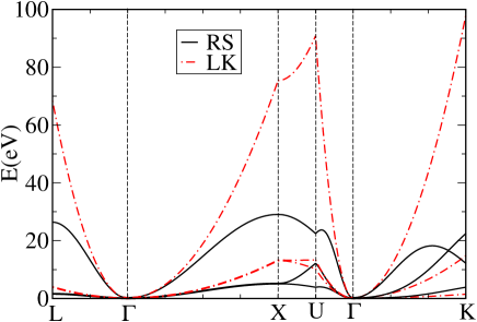
Figure 2: (color online) Band structure for GaAs obtained diagonalizing Eq.(10) (continuous lines). The dashed lines indicate the results for the Luttinger-Kohn model.

As expected, the bottom of the band is at $\Gamma$ and we observe the heavy hole and light hole bands along the high symmetry lines in the Brillouin zone shown in the figures. Since we are using “hole” language the top of the electronic valence band appears here as the bottom of the “hole” valence band. The dashed lines are the eigenvalues of Eq.(A8) in Ref.macdonald, , i.e., the Luttinger-Kohn model results. In order to check the agreement with our results around the point $\Gamma$ we shifted our curves by the value $8t_{xx}^{\parallel}+4t_{xx}^{\perp}$ so that the bottom of our valence band is at zero. It can be seen that the agreement between the curves obtained with our tight binding model and the Luttinger-Kohn ones is excellent at the $\Gamma$ point of the valence band. However, our model captures better the band dispersion away from the center of the Brillouin zone and the agreement with ARPES results is remarkable.ARPES

When $J\neq 0$ and a finite number of magnetic impurities are considered, the diagonalization of Eq.(31) has to be performed in real space. In Fig.3 we show the discrete energy eigenvalues along the high symmetry lines in the FBZ obtained numerically diagonalizing Eq.(31) using finite clusters (still with $J=0$). $N=N_{x}=N_{y}=N_{z}$ indicates the number of unit cells considered along each spatial direction.

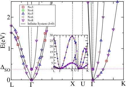
Figure 3: (color online) Band structure for GaAs obtained diagonalizing Eq.(10) (black lines). The symbols indicate results obtained using finite lattices in real space diagonalizing Eq.(31) with J=0. As the lattice size increases, more momentum states in the First Brillouin zone become available. The number of momentum states available inside the FBZ is given by $4N^{3}$.

Numerically, we study clusters that contain $N$ cubes of side $a_{0}$ along each of the 3 spatial directions. Since there are 4 ions associated to each site of the cube in an fcc lattice, the total number of Ga ions in the numerical simulation is given by $N_{Ga}=4N^{3}$. This means that there is an equal number of points inside the FBZ in momentum space. As already mentioned, the discrete lattice in momentum space is cubic. The side of the smallest cube is given by $b=2\pi/Na_{0}$ which is the size of the mesh corresponding to $N$ cubic cells along each of the three spatial directions. The first Brillouin zone has the shape of a truncated octahedron defined by well known high symmetry points such as $L=(\pi/a_{0},\pi/a_{0},\pi/a_{0})$, $X=(2\pi/a_{0},0,0)$, $U=(2\pi/a_{0},\pi/2a_{0},\pi/2a_{0})$, $K=(3\pi/2a_{0},3\pi/2a_{0},0)$, etc.equiv

The finiteness of the lattices imposes a constraint on the minimum Mn concentrations that can be reached: values of $x$ larger than 0.2% can be studied in lattices with $N=4$, i.e. 256 sites. The results presented in this work have been obtained using standard Monte Carlo simulations for the localized spins configurations which requires, at each iteration, the exact diagonalization of a $4N^{3}N_{o}\times 4N^{3}N_{o}$ fermionic matrix, where $N_{o}=6$ for Eq.(31) and 8 when the “$d$-orbital” is included.manga Using state-of-the-art computers such as the Cray XT3 supercomputer at ORNL we are currently able to perform production runs for $N=4$ and some runs with $N=5$ and 6, and also study non cubic lattices, to monitor finite size effects. We are working on adapting newly developed (approximated) numerical techniques such as the TPEM approachfuru to this problem with the hope of achieving production runs for $N=6$ and 8.

VI.1 Four Band Approximation

In the case of III-V semiconductors with strong spin-orbit interaction, i.e., large $\Delta_{SO}$ such as GaAs and GaSb, only the four $j=3/2$ orbitals are often considered to study the top of the valence band. macdonald ; KL This approximation would certainly simplify numerical simulations since the number of degrees of freedom per lattice site is reduced from six to four.

However, we have found an important drawback. As it can be seen in Fig.4 the band dispersions under the four-orbital approximation (continuous line) agrees with the dispersions for the six-orbital case (dashed line) only in a very small region about $\Gamma$ with radius $\delta ka_{0}\approx 0.02\pi$ while the study of many representative dopings such as $x=8.5\%$ with $p=0.7$ involves states at a radius $\delta ka_{0}\approx 0.5\pi$. In this situation the four-orbital approximation no longer holds. Along the $\Gamma-L$, $\Gamma-X$, and $\Gamma-U$ directions the heavy-hole dispersion is well reproduced for a large momentum range but the very close in energy light-hole state is not captured by the 4 orbital approximation. Even worse, along the $\Gamma-K$ direction, the flatness characteristic of the heavy-hole band is missed in the 4 orbital approach. Thus, the 4 orbital model would only be adequate to describe very lightly doped cases (probably in the insulating regime) beyond the reach of finite lattice simulations and not very relevant for the high $T_{C}$ regime.

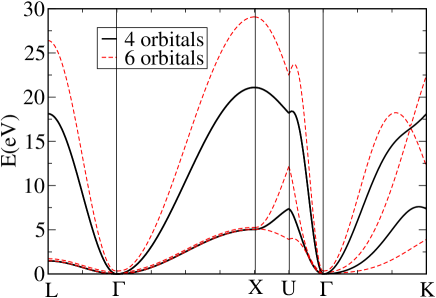
Figure 4: (color online) Band structure for GaAs obtained diagonalizing Eq.(10) (dashed lines). The band structure using the 4 orbital approximation is indicated with continuous lines.

An example of the shortcomings of the 4 orbital model is the incorrect form of the magnetization M as a function of temperature (T) that it provides. In Fig.5a the magnetization curve for $x=8.5\%$ Mn doped GaAs calculated with the 4-orbital approximation (circles) is compared with the one given by Eq.(31) (diamonds). The Curie-Weiss (CW) shape observed in experimentsPot is only captured by the 6-orbital modelwe while the 4-orbital approximation reproduces the concave shape observed in previous numerical efforts dealing mostly with single orbital models.Gonz ; Ken In addition, the value of $T_{C}$ is underestimated in this approach.

VI.2 Spin-Orbit Interaction

As pointed out in the previous subsection, a problem of early unbiased numerical efforts was the failure to reproduce the Curie-Weiss shape of the magnetization curves obtained in experiments of Mn doped GaAs with low compensation. While this shape was characteristic of most mean-field based approachesdietl00 ; macdonald , a concavity consistent with percolative behavior was observed otherwise.Gonz ; Ken

According to our results the CW behavior is very sensitive to the dispersion curves and the number of orbitals. Numerical simulations of the model presented here have shown that the spin-orbit interaction is crucial to obtain the CW shape of the magnetization curves.we In Fig.5a we present magnetization curves obtained in lattices with 256 Ga ions for $J=1.2eV$, $x=8.5\%$, and the hole density $p=0.7$. The curve with $\Delta_{SO}=0.34eV$, indicated with diamonds, is in excellent agreement with the experimental data for Mn doped GaAs exhibiting CW behavior. It also provides an appropriate value of $T_{C}$. On the other hand, the curve with $\Delta_{SO}=0$ (indicated with squares), shows a linear increase of the magnetization below $T_{C}$.

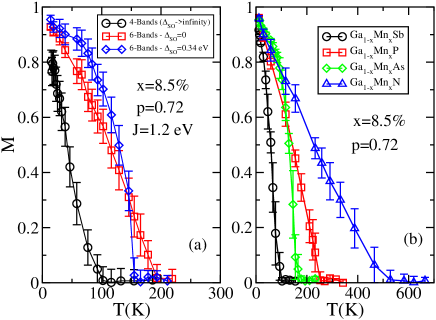
Figure 5: (color online) Magnetization vs temperature calculated numerically with x=8.5% of Mn, and a density of holes p=0.72 for (a) GaAs; the diamonds indicate the results with spin-orbit interaction while the squares show the points for which the spin-orbit interaction has been neglected. Results using the 4-orbital approximation, i.e. $\Delta_{SO}\rightarrow\infty$ are denoted by the circles. (b) GaSb (circles), GaAs (diamonds), GaP (squares), and GaN (triangles). The magnetization is measured as $\cal M=\sqrt{{\bf M}\cdot{\bf M}}$, with ${\bf M}$ the vectorial magnetization. As a consequence, for fully disordered spins, $\cal M$ is still nonzero due to the ${\bf S_{I}}^{2}$=1 contributions, causing a finite value at large temperatures (${\cal M}(T\to\infty)=1/\sqrt{xN_{Ga}}$) unrelated to ferromagnetism. Thus, we plotted ${\rm M}=({\cal M}-{\cal M}(T\to\infty))/(1-{\cal M}(T\to\infty))$, i.e. the background was subtracted.

We have also used Eq.(31) to calculate the magnetization of other doped III-V compounds with higher and lower spin-orbit coupling than GaAs. GaSb has a stronger spin-orbit coupling $\Delta_{SO}=0.75$eV. Eq.(31) can be used for GaSb with the hoppings obtained using Eq.(7) and (15) using the Luttinger parameters $(\gamma_{1},\gamma_{2},\gamma_{3})=(13.3,4.4,5.7)$.cardona $J$ is obtained using Eq.(30) and, since $a_{0}=6.10\AA$cardona , $J$=0.96eV.

The magnetization, denoted by the circles in Fig.5b shows CW behavior but $T_{C}\approx 100$K is lower than for GaAs at the same doping and compensation. The result roughly agrees with mean-field estimates.dietl00 We also present results for Mn doped GaP which has a much smaller spin-orbit coupling ($\Delta_{SO}=0.08$eV) than GaAs. The Luttinger parameters are $(4.05,0.49,1.25)$cardona and we use $J=1.34$eV. In this case we obtain a magnetization curve with an almost linear temperature dependence (squares in Fig.5b). This linear behavior has been obtained in measurements of (Ga,Mn)P with $1.8\%\leq x\leq 3.8\%$Farsh but it is not clear whether it will continue up to 8.5% doping if this value were reached.

For completeness, we also present the results for (Ga,Mn)N. A $T_{C}\approx 500$K, well above room temperature, is obtained in this case. This result is in agreement with mean-field predictions, assuming the doped Mn in the state Mn²⁺,dietl00 ; dietl02 ; mas and with some experimental measurements.gan ; Koro The effects of Mn-$d$-level participation will be discussed in subsection E.

VI.3 $J$-Induced Splitting of the Valence Band at the $\Gamma$-Point

Many studies of DMS are based on reasonable assumptions on the properties of the ground state. Some researchers work in the “high doping” regime assuming that the doped holes are uniformly distributed in the system and effectively doped into the valence band of the material. This is the so-called valence-band scenarioOHN96 ; dietl00 ; macdonald ; jung ; Sam in which the disorder configurations of the Mn ion are disregarded. The other approach, known as the impurity-band regime,IB considers the limit of very low doping in which the holes electrically bound to the impurity cores start forming an impurity band due to the overlap of the wave functions. In this case the disordered positions of the Mn ions would play an important role. Although each scenario must be valid in opposite doping regimes, it is not clear when the crossover between the two occurs (since it is a function of $x$, $J$, and other parameters) and which one better describes the experiments is controversial. Even for (Ga,Mn)As both descriptions are applied to the case of $x$=8.5%.

A way of shedding light on this issue is by studying the evolution as a function of $J$, and for different values of $x$, of the four degenerate states at the top of the valence band ($\Gamma$ point) of the parent compound. This splitting is due to the interaction of the doped holes with the localized spins and it was briefly described when the classical limit was discussed in section IV.A. For small values of $J$, at values of $x$ in the metallic regime according to Mott’s criterion, it is expected that the mean-field approach (assuming uniform hole distribution) should be a good approximation. The calculations indicateFurd ; Dietl ; Szc that the levels will split following a linear behavior in $Jx$, i.e., $E_{0}\pm B_{G}$ and $E_{0}\pm 3B_{G}$ with $B_{G}$ given in Eq.(23) and (24).

We have evaluated the eigenvalue distribution for different Mn disorder configurations (indicated with different symbols in Fig.6) as a function of $J$ for $x$=8.5% (Fig.6a) and 5% (Fig.6b). For both values of $x$ it can be seen that the mean-field prediction is accurate for $J\leq 0.5$eV; for $J$=1.2eV, i.e., the accepted value for GaAs, the eigenvalues have lower energies than the mean-field ones indicating a stronger distortion of the bands due to the interactions. However, the eigenvalues appear to be independent of the disorder configurations indicating that the holes are non-localized; this uniform hole distribution continues up to $J\approx 4$eV which is the value at which our numerical simulations indicate that an impurity band starts to develop in the density of states.we For larger values of $J$ there is a large spread in the eigenvalue distribution as a function of the disorder. Notice that the effects of disorder are much stronger for $x$=5% than for $x$=8.5% which corroborates the assumption that the role of disorder diminishes as $x$ increases. It is interesting to notice that, in disagreement with the mean-field expectation that the spread in the eigenvalue distribution should increase with $x$, we actually observe that as $x$ increases the width of the eigenvalues band decreases.

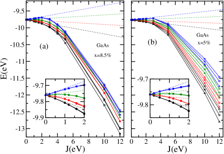
Figure 6: (color online) Numerically determined evolution of the four degenerate states at the top of the valence as a function of $J$ for (a) $x=0.085$ and (b) for $x=0.05$ in a 256 sites lattice. The different symbols indicate different Mn disorder configurations. The dotted lines correspond to the mean-field predictions. The insets show the range in $J$ for which agreement between the numerical and mean-field results occur.

These results indicate that $J=1.2$eV corresponds to an intermediate region in which in the metallic regime the holes are not localized (if in the metallic regime of $x$)but the mean-field approximation needs corrections.

VI.4 Dependence of $T_{C}$ with $x$

An important issue in DMS is the dependence of the Curie temperature with the amount of magnetic impurities. Mean-field calculationsmacdonald predict that $T_{C}$ increases linearly with $x$ but numerical simulations in simple systems indicate that $T_{C}$ reaches a maximum at an optimal value of $x$ ($x_{opt}$) and decreases afterwards.Gonz The optimal value of $x$ was found to be a function of $J$. For large $J$, $x_{opt}\rightarrow 1$ while $x_{opt}\approx 0.25$ for the values of $J$ that capture the physics of (Ga,Mn)As. Experimentally, in (Ga,Mn)As, $T_{C}$ has been found to increase with $x$ up to about $x$=10%.Pot Recently, $x$=12.2%- 21.3% has been achievedtanaka but the highest $T_{C}$ observed has been 170K, i.e., no higher than the record value ($T_{C}$=173K) obtained with $x$=9%.wang In fact, for both annealed and as grown samples it was observed that $T_{C}$ reaches a broad maximum for $x\sim$10%-15% and decreases afterwards. It is not clear whether the decrease is due to intrinsic properties of the material or to a larger amount of compensation. In Fig.7 we present results for $T_{C}$ vs $x$ obtained with Eq.(31) using the parameters for (Ga,Mn)As. Experimental points are presented for comparison. As $x$ increases longer thermalizations are needed in the numerical simulations. For $p=0.5$, 0.75 and 1 we have obtained reasonable agreement with the experimental data for the annealed samples. We obtained a maximum $T_{C}=(225\pm 20)$K for $x=12.5\%$ in the non-compensated case, i.e. $p=1$. Thus, according to our calculations, even larger Mn doping of GaAs would not allow to reach a Curie temperature above room temperature.

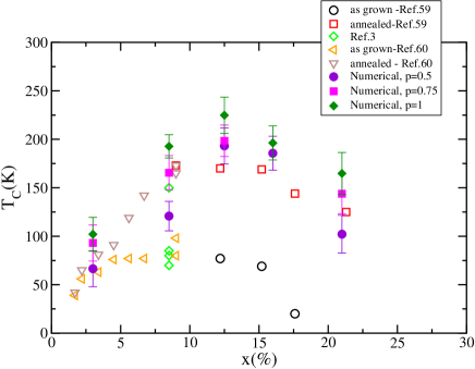
Figure 7: (color online) Numerically determined $T_{C}$ as a function of $x$ for $\rm{Ga_{\it 1-x}Mn_{\it x}As}$ for different values of compensation $p$. Experimental data are also shown.

VI.5 Coulomb Attraction at Mn Sites

Numerical calculations of the density of states (DOS) using Eq.(31) for the case of (Ga,Mn)As have indicated that the chemical potential is in the valence band for dopings x=3% or higher.we As discussed in Section V.A it has been argued by some researchers that this outcome may be the result of neglecting the effects of Coulomb attraction between the localized Mn²⁺ ions and the doped holes. In this subsection we will study the effects of adding the terms Eq.(32) and Eq.(33) to Eq.(31). In Ref.Popescu, it was estimated that $V=-1.9eV$ for Mn doped GaAs. In Fig.8 it can be seen that the DOS for both x=8.5% (Fig.8a) and 3% (Fig.8b) remains basically unchanged when either an onsite or a nearest neighbor Coulomb potential of the above magnitude is added. The chemical potential is still in the valence band and no hint of impurity band appears. Since even for the zero range potential the holes are already delocalized, there is no difference when the longer range potential is considered. Similar results (no IB in the DOS) are obtained for the case of (Ga,Mn)P using V=-2.4 eV.Popescu This indicates that for the values of the parameters for (Ga,Mn)As, the addition of Coulomb attraction is irrelevant in the range of doping of interest, i.e., x$\geq 3\%$.

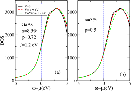
Figure 8: (color online) Numerically determined density of states for Mn doped GaAs with (a) $x=0.085$ and and $p=0.72$ and (b) for $x=0.05$ and $p=0.5$. The different lines indicate different ranges of the Coulomb potential. $Vnn$ indicates the value of the Coulomb potential at the impurity’s nearest neighbor sites.

However, for larger (but unphysical) values of $J$ our results confirm the conclusions of Ref.Popescu, regarding the importance of considering a nearest-neighbor range potential in order to accurately obtain the value of $x$ for which the crossover between the IB and VB description occurs. In Fig.9 we show the DOS for the unphysical case in which the hopping parameters correspond to GaAs but we set $J$=7eV instead of the realistic value 1.2eV for x=8.5% (dashed line in Fig.9). We chose $J$=7 eV because it is close to the value for which a clearly separated IB develops in the DOS.we By adding an on-site Coulomb potential of strength -3.5eV an IB develops (continuous line) and the chemical potential is located there. Clearly the holes are trapped at the Mn sites due to the large potential. However, if a nearest-neighbor range potential with the same strength is applied, the holes become delocalized and the IB band in the DOS disappears (dot-dashed line).

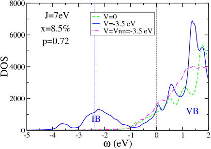
Figure 9: (color online) Numerically determined density of states for $J=7$eV with x=8.5%. For $V=0$ (dashed line), on site $V$=-3.5 eV (continuous line), and nearest-neighbor range $V$=-3.5 eV (dot-dashed line).

The above result indicates that studies of the crossover from impurity to valence band regimes performed with on-site rather than extended attractive potentials will overestimate the range of the impurity band regime.

VI.6 Mn $d$-orbitals

Finally, in this subsection, we will consider the possibility of Mn³⁺ doping in some III-V compounds such as GaN.

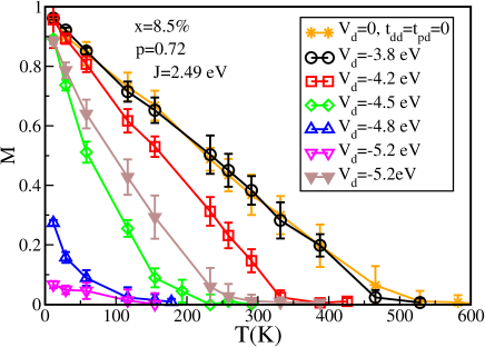
Figure 10: (color online) Numerically determined magnetization vs $T$ for Mn doped GaN with phenomenological $d$ orbitals. The open symbols correspond to $t_{dd}=-0.1eV$ and $t_{pd}=0.1eV$ while the close symbols indicate $t_{dd}=0.5eV$ and $t_{pd}=0.5eV$. The stars are data for the 6-orbital model.

In Fig.10 the stars indicate the magnetization as a function of temperature obtained using the six-orbital Hamiltonian in Eq.(31) with the parameters for GaN on a 256 sites lattice which has already been presented in Fig.5. For this material some experimentsGraf ; Kreis and calculationsKro ; Thomas ; Kula suggest that Mn $d$-levels may not be deep into the valence band. Thus, Mn³⁺, instead of Mn²⁺, may be present. To explore the consequences of this possibility we will use the 8-orbital model that results from the addition of Eq.(34) to Eq.(31). As mentioned in Section V.B the relative position of the $d$ level $V_{d}$ and the $d-d$ and $d-p$ hoppings will be input parameters. First, we will consider the case in which the hoppings involving the $d$-orbitals are smaller than the hoppings among $p$-orbitals. Fixing $t_{dd}=-0.1$eV and $t_{pd}=0.1$eV, we present the magnetization vs T for various values of $V_{d}$ indicated in Fig.10 (open symbols). For $V_{d}=-3.8$eV, which corresponds to the $d$-orbitals deep into the valence band (open circles), the results are similar to the ones obtained for the 6-orbital case as expected. However, as $V_{d}$ becomes more negative indicating that the $d$-level moves into the gap it can be clearly seen that both the magnetization and $T_{C}$ decrease. However, it is important to notice that, even in the case of $d$-orbitals in the gap, the magnetization and $T_{C}$ increase if the hoppings between $d$ and $p$ orbitals are allowed to be larger. For example, for $|t_{pd}|=|t_{dd}|=0.5$eV and $V_{d}=-5.2$eV, indicated with filled triangles in Fig.10, the Curie temperature becomes very close to room temperature. This behavior is in agreement with the ab initio results of Ref.Kro, .

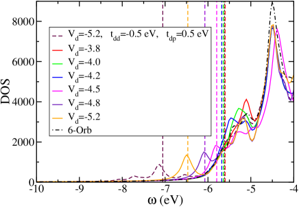
Figure 11: (color online) Numerically determined DOS for Mn doped GaN with phenomenological d orbitals. The continuous lines correspond to $t_{dd}=-0.1eV$ and $t_{pd}=0.1eV$ for the values of $V_{d}$ indicated while the dashed line indicates $t_{dd}=0.5eV$ and $t_{pd}=.5eV$. Data for the 6-orbital model are denoted with dashed-dotted line.

$T_{C}$ is related to the band structure as it can be seen in Fig.11. As $|V_{d}|$ becomes larger an impurity band develops in the DOS. When $t_{pd}<<t_{pp}$ the IB has very small dispersion indicating that the trapped holes are very localized. When $t_{pd}$ increases the IB acquires dispersion and $T_{C}$ becomes higher.

VII Conclusions

We have presented a Hamiltonian that enables the numerical study of the physics of DMS with an equally accurate treatment of both the kinetic and magnetic interactions. Provided that the parent compound is a Zinc-Blende type semiconductor for which the Luttinger parameters are known, there are no arbitrary parameters in the Hamiltonian. Only 6 orbitals per site have to be considered to obtain accurate Curie temperatures and magnetization curves of materials where Mn²⁺ is present, which makes possible to perform numerical simulations in large systems with present day computers. Besides reproducing well established experimental results for GaAs with less than 10% Mn doping, the higher doping regime was explored. While naively it could have been expected that $T_{C}$ would increase continuously with $x$, we observed that it reaches a maximum value at an intermediate value of the doping. For GaAs we found that the highest value of $T_{C}$, approximately 220K, occurs $x$=12.5% and no compensation, indicating that higher doping of GaAs will not lead to $T_{C}$’s above room temperature. The doping for which the maximum $T_{C}$ occurs appears to be in general agreement with recent experimental results.

The possibility of Mn³⁺ doping in GaP or GaN has been considered phenomenologically. We found that $T_{C}$ will be very reduced if the $d$ levels are located at energies much higher than the top of the valence band and if the $pd$ hybridization is weak. However, if the hybridization is strong, Mn doped GaN could be a good candidate for high $T_{C}$.

It has also been shown that the Coulomb attraction between the hole and the Mn ions expected at low doping does not play a role for $x$ larger than 3% in GaAs. As a consequence, we have not observed an impurity band that should be present at lower dopings or even in the metallic regime if the magnetic interaction were stronger.The relative weakness of the magnetic interaction was confirmed by studying the splitting of the top of the valence band as a function of $J$. For values of $J$ within the experimental range for Mn doped GaAs, we have observed a departure from the mean-field predictions. However, the holes do not appear to be localized at the Mn impurity sites since the eigenvalue distribution is independent of the particular disorder configuration. Localization is observed only at unrealistically high values of $J$.

Summarizing, we have shown that the real space Hamiltonian presented here reproduces the top of the valence band given by the Luttinger-Kohn model for the undoped parent compounds and, as such, it is guaranteed to provide an excellent framework for the numerical study of lightly doped Zinc-blende type magnetic semiconductors.

VIII Acknowledgments

We acknowledge discussions with E. Dagotto, T. Schulthess, F. Popescu and J. Moreno. Y.Y. and A.M. are supported by NSF under grants DMR-0706020. This research used resources of the NCCS. G.A. is sponsored by the Division of Scientific User Facilities and the Division of Materials Sciences and Engineering, BES, DOE, contract DE-AC05-000R22725 with ORNL, managed by UT-Battelle.

IX Appendix I

Here we provide the change of basis matrices used in Eq.(12) and (13).

$$M=\left(\begin{array}[]{cccccc}-{1\over{\sqrt{2}}}&-{i\over{\sqrt{2}}}&0&0&0&0\\ {1\over{\sqrt{6}}}&-{i\over{\sqrt{6}}}&0&0&0&\sqrt{{2\over{3}}}\\ 0&0&\sqrt{{2\over{3}}}&{-1\over{\sqrt{6}}}&{-i\over{\sqrt{6}}}&0\\ 0&0&0&{1\over{\sqrt{2}}}&-{i\over{\sqrt{2}}}&0\\ 0&0&-{1\over{\sqrt{3}}}&-{1\over{\sqrt{3}}}&-{i\over{\sqrt{3}}}&0\\ -{1\over{\sqrt{3}}}&{i\over{\sqrt{3}}}&0&0&0&{1\over{\sqrt{3}}}\end{array}\right)$$

and its inverse $M^{-1}$ is

$$M^{-1}=\left(\begin{array}[]{cccccc}-{1\over{\sqrt{2}}}&{1\over{\sqrt{6}}}&0&0&0&-{1\over{\sqrt{3}}}\\ {i\over{\sqrt{2}}}&{i\over{\sqrt{6}}}&0&0&0&{-i\over{\sqrt{3}}}\\ 0&0&\sqrt{{2\over{3}}}&0&{-1\over{\sqrt{3}}}&0\\ 0&0&{-1\over{\sqrt{6}}}&{1\over{\sqrt{2}}}&{-1\over{\sqrt{3}}}&0\\ 0&0&{i\over{\sqrt{6}}}&{i\over{\sqrt{2}}}&{i\over{\sqrt{3}}}&0\\ 0&\sqrt{{2\over{3}}}&0&0&0&{1\over{\sqrt{3}}}\end{array}\right)$$

References

- (1) H. Ohno, Science 281, 951 (1998).
- (2) T. Dietl, H. Ohno, F. Matsukura, J. Cibert, D. Ferrand, Science, 287, 1019 (2000).
- (3) S. J. Potashnik, K.C. Ku, S.H. Chun, J.J. Berry, N. Samarth, and P. Schiffer, Appl. Phys. Lett. 79, 1495 (2001).
- (4) I. Zutic,J. Fabian, and S. Das Sarma, Rev. Mod. Phys. 76, 323 (2004).
- (5) Peter Yu and Manuel Cardona, “Fundamentals of Semiconductors”, Third Edition, Springer-Verlag.
- (6) J.M. Luttinger and W. Kohn, Phys.Rev.97, 869 (1955).
- (7) M. Abolfath, T. Jungwirth, J. Brum and A. MacDonald, Phys. Rev. B63 054418 (2001).
- (8) T. Dietl, H.Ohno and F. Matsukura, Phys.Rev.B63, 195205 (2001).
- (9) G. Alvarez, M. Mayr, and E. Dagotto, Phys. Rev. Lett. 89, 277202 (2002).
- (10) M. Mayr, G.Alvarez, and E. Dagotto, Phys. Rev. B 65, 241202(R) (2002).
- (11) M. Kennett, M. Berciu, and R. N. Bhatt, Phys. Rev. B 66, 045207 (2002).
- (12) S. Das Sarma, E.H. Hwang, and A. Kaminski , Phys. Rev. B 67, 155201 (2003).
- (13) J. Schliemann, Jürgen König, and A.H. MacDonald, Phys. Rev. B 64, 165201 (2001).
- (14) J. Xu, M. van Schilfgaarde, and G.D. Samolyuk, Phys. Rev. Lett. 94, 097201 (2005).
- (15) W.A. Harrison, Phys.Rev.B8, 4487 (1973).
- (16) Y.-C. Chang, Phys.Rev.B37, 8215 (1987).
- (17) J.C. Slater and G.F. Koster, Phys. Rev. 94, 1498 (1954).
- (18) J. Okabayashi, A. Kimura, O. Rader, T. Mizokawa, A. Fujimori, T. Hayashi and M. Tanaka, Phys.Rev.B58, R4211 (1998).
- (19) J.M. Luttinger, Phys.Rev.102, 1030 (1956).
- (20) Similar expressions were obtained in Ref.chang, .
- (21) The sign of the diagonal hoppings determines whether the band is hole-like or electron-like. The sign of the interorbital hopping does not affect the shape of the band that only depends on the absolute value of this hopping.
- (22) These expressions are implicit in Eq.(6) of Ref.chang, .
- (23) J. Szczytko,A. Twardowski, K. Swiatek, M. Palczewska, M. Tanaka, T. Hayashi, and K. Ando, Phys. Rev.B60, 8304 (1999); O.M. Fedorych, E. M. Hankiewicz, Z. Wilamowski, and J. Sadowski, Phys.Rev.B66, 045201(2002).
- (24) M. Linnarsson, E. Janzen, and B. Monemar, Phys.Rev.B55, 6938 (1997).
- (25) F. Matsukura, H. Ohno, A. Shen, and Y. Sugawara, Phys.Rev.B57, R2037 (1998).
- (26) M. Troyer and U.-J. Wiese, Phys.Rev.Lett.94, 170201 (2005).
- (27) Y. Yildirim, G. Alvarez, A. Moreo, and E. Dagotto, Phys. Rev. Lett.99, 057207 (2007).
- (28) G. Q. Pellegrino, K. Furuya, and M.C. Nemes, Chaos 5 463 (1995); G.Q. Pellegrino, K. Furuya, and M.C. Nemes, Revista Brasileira de Ensino de Fisica 20, 321 (1998); L.G. Yaffe, Rev. Mod. Phys. 54, 407 (1982).
- (29) J. Szczytko, W. Bardyszewski, and A. Twardowski, Phys.Rev. B64, 075306 (2001).
- (30) J.K. Furdyna, J. Appl. Phys.64, R29 (1988).
- (31) J.I. Hwang, Y. Ishida, M. Kobayashi, H. Hirata, K. Takubo, T. Mizokawa, A. Fujimori, J. Okamoto, K. Mamiya, Y. Saito, Y. Muramatsu, H. Ott, A. Tanaka, T. Kondo,and H. Munekata, Phys.Rev.B72, 085216 (2005); A. Wolos, M. Palczewska, M. Zajac, J. Gosk, M. Kaminska, A. Twardowski, M. Bockowski, I. Grzegory, and S. Porowski, ibid B69, 115210 (2004).
- (32) J. Schneider, U. Kaufmann, W. Wilkening, M. Baeumler, and F. Köhl, Phys. Rev. Lett. 57, 240 (1987).
- (33) V. Fleurov, K. Kikoin, V.A. Ivanov, P.M. Krstajic, and F.M. Peeters,J. of Magnetism and Magnetic Mat.272-276 1967 (2004).
- (34) F. Popescu, C. Sen, E. Dagotto, and A. Moreo, Phys. Rev. B76, 085206 (2007).
- (35) R. Y. Korotkov, J. M. Gregie, and B. W. Wessels J. Appl. Phys. Letts.80, 1731 (2002).
- (36) J. Kreissl, W. Ulrici,M. El-Metoui, A.-M. Vasson, A. Vasson, and A. Gavaix , Phys. Rev. B54, 10508 (1996).
- (37) Leeor Kronik, Manish Jain, and James R. Chelikowsky, Phys. Rev. B60, 041203(R) (2002).
- (38) T. Graf, M. Gjukic, M.S. Brandt, and M. Stutzmann, Appl. Phys. Lett. 81, 5159 (2002).
- (39) A. K. Bhattacharjee and C.B. à la Guillaume, Solid State Commun. 113, 17 (2000).
- (40) S. Pantelides, Rev. Mod. Phys 50, 797 (1978).
- (41) M. Takahashi and K. Kubo, J. Phys. Soc. Jpn. 72, 2866 (2003).
- (42) M. Calderón, G. Gómez-Santos, and L. Brey, Phys. Rev. B 66, 075218 (2002).
- (43) E.H. Hwang and S. Das Sarma, Phys. Rev. B 72, 035210 (2005).
- (44) T. Dietl, cond-mat/0703278.
- (45) J. Tworzydlo, Phys. Rev. B 50, 14591 (1994).
- (46) C.Y. Fong, V.A. Gubanov and C. Boekema, J. Electron. Mater. 29, 1067 (2000); M. van Schilfigaarde and O.N. Myrasov, Phys.Rev.B63, 233205 (2001).
- (47) P.M. Krstajic, F. M. Peeters, V. A. Ivanov, V. Fleurov, and K. Kikoin, Phys.Rev.B70, 195215 (2004).
- (48) J.Okabayashi, A. Kimura, O. Rader, T. Mizokawa, A. Fujimori, T. Hayashi, and M. Tanaka, Physica E10, 192 (2001).
- (49) Notice that although and are equivalent points in terms of the FBZ the path between these two points and is not the same and the bands dispersion along the two directions are very different.
- (50) E. Dagotto, T. Hotta, and A. Moreo, Phys. Rep. 344 1 (2001)).
- (51) Y. Motome and N. Furukawa, J. Phys. Soc. Jpn.68, 3853 (1999); N. Furukawa, Y. Motome, and H. Nakata, Computer Physics Communications 142, 410 (2001); N. Furukawa and Y. Motome, J. Phys. Soc. Jpn. 73, 1482 (2004); Y. Motome and N. Furukawa, Phys. Rev. B68, 144432 (2003).
- (52) R. Farshchi, M.A. Scarpulla, P.R. Stone, K.M. Yu, I.D. Sharp, J.W. Beeman, H.H. Silvestri, L.A. Reichertz, E.E. Haller, and O.D. Dubon, Sol. State. Comm.140 443 (2006).
- (53) T. Dietl, F. Matsukura, and H. Ohno, Phys. Rev. B66, 033203 (2002).
- (54) J. Masek, J. Kurrnovsky, F. Maca, J. Sinova, A. MacDonald, R. Campion, B. Gallagher, and T. Jungwirth, cond-mat/0609158.
- (55) S. Yoshii, S. Sonoda, T. Yamamoto, T. Kashiwagi, M. Hagiwara, Y. Yamamoto, Y. Akasaka, K. Kindo, and H. Hori, cond-mat/0604647.
- (56) T. Jungwirth, J. Sinova, J. Maček, J. Kučera, and A.H. MacDonald, Rev. Mod. Phys. 78, 809 (2006).
- (57) A.H. MacDonald, P. Schiffer, N. Samarth, Nature Materials 4, 195 (2005).
- (58) M. Berciu and R. Bhatt, Phys. Rev. Lett. 87, 107203 (2001); H. Akai, Phys. Rev. Lett. 81, 3002 (1998).
- (59) Shinobu Ohya, Kenichi Ohno and Masaaki Tanaka, Appl. Phys. Lett. 90, 112503 (2007).
- (60) K.Y. Wang, R. Campion, K. Edmonds, M. Sawicki, T. Dietl, C. Foxon, and B. Gallagher, AIP Conf. Proc.772, 333 (2005); T. Jungwirth, K. Y. Wang, J. Maek, K. W. Edmonds, Jürgen König, Jairo Sinova, M. Polini, N. A. Goncharuk, A. H. MacDonald, M. Sawicki, A. W. Rushforth, R. P. Campion, L. X. Zhao, C. T. Foxon, and B. L. Gallagher, Phys.Rev. B72, 165204 (2005).
- (61) T. Schulthess, W. Temmerman, Z. Szotek, W. Butler, and M. Stocks, Nature Materials 4, 838 (2005).
- (62) E. Kulatov, H. Nakayama, H. Mariette, H. Ohta, and Yu. Uspenskii, Phys. Rev. B66, 045203 (2002).