Electron-phonon coupling and longitudinal mechanical-mode cooling in a metallic nanowire

Abstract

We investigate electron-phonon coupling in a narrow suspended metallic wire, in which the phonon modes are restricted to one dimension but the electrons behave three-dimensionally. Explicit theoretical results related to the known bulk properties are derived. We find out that longitudinal vibration modes can be cooled by electronic tunnel refrigeration far below the bath temperature provided the mechanical quality factors of the modes are sufficiently high. The obtained results apply to feasible experimental configurations.

Electron-phonon coupling in metals, albeit extensively studied over several decades gantmakher74 , is of utmost interest and importance in view of present day developments in nanoelectromechanics cleland03 ; schwab05 and in electronic cooling and sensing on nanoscale giazotto06 ; saira07 . A number of questions arise when the dimensionality of the phonons is reduced from the conventional bulk three-dimensional case qu05 ; yu95 ; kuhn06 . Recent experimental observations of metallic wires on thin dielectric membranes support the fact that reduction of phonon dimensionality leads to weaker temperature dependence of the heat flux between electrons and phonons karvonen07 . Very little is known about truly one-dimensional wires, where transverse dimensions are far smaller than the thermal wavelength of the phonons, although this regime is readily available experimentally at sub-kelvin temperatures in wires whose diameter is of the order of 100 nm or less. Recently though, substantial overheating was conjectured to be the origin of excess low-frequency charge noise in a suspended single-electron transistor in this particular one-dimensional geometry li07 . In this Letter we derive an explicit result for electron-phonon heat flux in a metallic wire in which electrons behave three-dimensionally but phonons are confined to one dimension, and relate this result to the standard bulk result for the corresponding metal. We present a scenario of tunnel coupling the metal electrons in a wire to a superconductor on bulk, whereby cooling of wire electrons can be realized. We demonstrate that the few available mechanical modes, i.e., discrete longitudinal phonons, can be cooled significantly by their coupling to the cold electrons in the wire. This occurs provided the mechanical modes are not too strongly coupled to the thermal bath, meaning that the mechanical $Q$ value of the mode is sufficiently high. Recently, indirect experimental evidence of electronic cooling of phonons in a bulk system was put forward in Ref. rajauria07 .

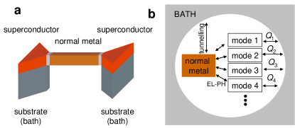
Figure 1: The system under study. In (a) we show the suspended wire whose transverse dimensions are supposed to be smaller than the thermal wavelength of the phonons, $\lambda_{\rm thermal}$. In this particular example the metal wire is connected to the bulk superconducting reservoirs via tunnel barriers to form a tunnel junction refrigerator. In (b) we show the relevant thermal model of the system.

To obtain results for the electron-phonon heat flux in a one-dimensional metallic wire (see Fig. 1 for the geometry and thermal model), we follow the standard procedure from the existing literature normally applied to the case of either bulk three-dimensional phonons gantmakher74 ; wellstood94 , or to the case where phonons are restricted to a semi-infinite bulk qu05 . The net heat flux from electrons into a discrete phonon mode $\mu$ at wave vector ${\bf q}$ is given by

$$\dot{Q}_{e\rightarrow\mu}({\bf q})=2\sum_{\bf k}\hbar\omega_{\mu}[\Gamma^{\rm e}_{\mu}({\bf k}\rightarrow{\bf k-q})-\Gamma^{\rm a}_{\mu}({\bf k}\rightarrow{\bf k+q})],$$ (1)

where phonon emission (e) and absorption (a) rates by the electrons with wave vector ${\bf k}$ are obtained via the golden rule as

$$\Gamma^{\rm e}_{\mu}({\bf k}\rightarrow{\bf k-q})=\frac{2\pi}{\hbar}|g_{\mu,\bf q}|^{2}[n(\frac{\hbar\omega_{\mu}}{k_{B}T_{\mu}})+1]$$

$$\times f(E_{\bf k})[1-f(E_{\bf k-q})]\delta(E_{\bf k}-E_{\bf k-q}-\hbar\omega_{\mu}),$$ (2)

and

$$\Gamma^{\rm a}_{\mu}({\bf k}\rightarrow{\bf k+q})=\frac{2\pi}{\hbar}|g_{\mu,\bf q}|^{2}n(\frac{\hbar\omega_{\mu}}{k_{B}T_{\mu}})$$

$$\times f(E_{\bf k})[1-f(E_{\bf k+q})]\delta(E_{\bf k}-E_{\bf k+q}+\hbar\omega_{\mu}).$$ (3)

Here $g_{\mu,\bf q}$ and $n(\frac{\hbar\omega_{\mu}}{k_{B}T_{\mu}})=[\exp(\frac{\hbar\omega_{\mu}}{k_{B}T_{\mu}})-1]^{-1}$ are the electron-phonon coupling constant and the Bose distribution, respectively, of the phonon mode $\mu$ at angular frequency $\omega_{\mu}$ and at temperature $T_{\mu}$, and $f(E)=[\exp(\frac{E}{k_{B}T_{e}})+1]^{-1}$ is the Fermi distribution of the electrons at temperature $T_{e}$.

We next evaluate $g_{\mu,\bf q}$ using the standard results of deformation potential of the collective lattice vibrations cleland03 . Let ${\bf w}_{\mu}({\bf r})$ be the displacement vector for mode $\mu$ normalized in the volume of the wire, $\mathcal{V}$, such that $\int d^{3}{\bf r}\,\,{\bf w}_{\mu}({\bf r}){\bf\cdot}{\bf w}_{\mu^{\prime}}^{*}({\bf r})=\delta_{\mu\mu^{\prime}}$. Then $g_{\mu,\bf q}$ can be obtained from the divergence of ${\bf w}_{\mu}({\bf r})$

$$g_{\mu,\bf q}=\frac{2}{3}E_{F}\sqrt{\frac{\hbar}{2\rho\omega_{\mu}}}\int d^{3}{\bf r}\,\,\Psi_{\bf k-q}({\bf r})\Psi_{\bf k}^{\dagger}({\bf r})\,\,\nabla\cdot{{\bf w}_{\mu}({\rm r})},$$ (4)

where $\Psi_{\bf k}({\bf r})$ are the electronic wave functions. Here $E_{F}$ is the Fermi energy of the electrons and $\rho$ is the mass density of the wire.

The thermal wavelength of phonons, $\lambda_{\rm thermal}=\frac{hc_{\ell}}{k_{B}T}$ at temperature $T$ and mode velocity $c_{\ell}$ is typically of order 1 $\mu$m at $T=100$ mK. In a wire whose length $L>\lambda_{\rm thermal}$ and with transverse dimensions $\ll\lambda_{\rm thermal}$, only modes with ${\bf q}=(0,0,q)$ directed along the wire ($z$-axis) appear relevant, since the ones with perpendicular ${\bf q}$ are too high in energy. There are basically four types of vibrations: longitudinal, flexural (two, with $x$ and $y$ polarizations), torsional and shear modes rego98 . The last one has a gap and is therefore not excited at low temperatures. Of the remaining ones the torsional modes have no divergence, and essentially only the longitudinal modes couple to electrons in the long wavelength limit. Experimentally this seems to be the case in carbon nanotubes sapmaz06 .

We consider longitudinal modes with specific boundary conditions: the wire (or the three-dimensional body) is assumed to be clamped at the ends. As we will detail below, this corresponds to a feasible realization. Let the wire extend from $z=0$ to $z=L$. Then, the normalized longitudinal eigenmodes of the beam are given by

$${\bf w}_{\mu}({\bf r})=\sqrt{\frac{2}{\mathcal{V}}}\sin(\mu\pi z/L)\hat{\bf z}\mbox{, }\mu=1,2,3,\ldots$$ (5)

They are characterized by the linear dispersion relation $\omega_{\mu}=c_{\ell}\mu\pi/L$, where $c_{\ell}=\sqrt{E/\rho}$ is the longitudinal sound velocity ($E$ is Young’s modulus). Assuming zero electronic boundary conditions along with equal electronic and phononic volumes we obtain again in the long wavelength limit

$$|g_{\mu,\bf q}|^{2}=\frac{1}{9}\frac{\hbar E_{F}^{2}q^{2}}{\rho\mathcal{V}\omega_{\mu}}\delta_{q,q_{\mu}}\equiv\mathcal{M}_{\ell}^{2}q\delta_{q,q_{\mu}},\,\,q_{\mu}=\mu\pi/L,$$ (6)

where $\mathcal{M}_{\ell}^{2}\equiv\frac{1}{9}\frac{\hbar E_{F}^{2}}{\rho\mathcal{V}c_{\ell}}$. The momentum $q$ transferred between the electron and the vibrational modes of a clamped beam takes discrete values $q_{\mu}$ only and is by convention positive.

We perform next the integration over electron energies in Eqs. (Electron-phonon coupling and longitudinal mechanical-mode cooling in a metallic nanowire) and (Electron-phonon coupling and longitudinal mechanical-mode cooling in a metallic nanowire) and insert the results in Eq. (1) obtaining

$$\dot{Q}_{e\rightarrow\mu}(q_{\mu})=\frac{2\pi\mathcal{M}_{\ell}^{2}c_{\ell}^{2}mN(E_{F})}{\hbar k_{F}}q_{\mu}^{2}[n(\frac{\hbar c_{\ell}q_{\mu}}{k_{B}T_{e}})-n(\frac{\hbar c_{\ell}q_{\mu}}{k_{B}T_{\mu}})].$$ (7)

Here, $m$ is the electron mass, $k_{F}$ the Fermi wave vector, and $N(E_{F})$ the electronic density of states at the Fermi energy. Three-dimensional distribution of electrons was assumed here, since we discuss only the case of ordinary metals, where $k_{F}^{-1}\ll 1$ nm. Using the definition of $\mathcal{M}_{\ell}^{2}$ above, and $N(E_{F})=\frac{mk_{F}\mathcal{V}}{\pi^{2}\hbar^{2}}$ and $E_{F}=\frac{\hbar^{2}k_{F}^{2}}{2m}$ of the free electron gas, the prefactor in Eq. (7) can also be written in the form $\frac{2\pi\mathcal{M}_{\ell}^{2}c_{\ell}^{2}mN(E_{F})}{\hbar k_{F}}=\frac{1}{18\pi}\frac{\hbar^{2}k_{F}^{4}c_{\ell}}{\rho}$. The total heat flux between electrons and phonons can then be obtained as a sum over all modes:

$$\dot{Q}_{e\rightarrow p}=\sum_{\mu}\dot{Q}_{e\rightarrow\mu}(q_{\mu}).$$ (8)

We obtain the continuum result for a long $L\gg\lambda_{\rm thermal}$ 1D wire by assuming a uniform density of modes with all of them at the same temperature $T_{\mu}=T_{p}$. We then replace the sum by an integral, $\sum_{q}\rightarrow\frac{L}{\pi}\int_{0}^{\infty}dq$. After a straightforward integration we obtain

$$\dot{Q}_{e\rightarrow p}=\Sigma_{\rm 1D}L(T_{e}^{3}-T_{p}^{3}).$$ (9)

Here, $\Sigma_{\rm 1D}$ is given by

$$\Sigma_{\rm 1D}=\frac{\zeta(3)}{18\pi^{2}}\frac{k_{F}^{4}k_{B}^{3}}{\hbar c_{\ell}^{2}\rho}.$$ (10)

It is instructive to compare this result to the celebrated result for longitudinal phonons in three dimensions (see, e.g., wellstood94 and references therein)

$$\dot{Q}_{e\rightarrow p}=\Sigma\mathcal{V}(T_{e}^{5}-T_{p}^{5}).$$ (11)

Here, the material specific prefactor $\Sigma$ is given by:

$$\Sigma=\frac{\zeta(5)}{3\pi^{3}}\frac{k_{F}^{4}k_{B}^{5}}{\hbar^{3}c_{\ell}^{4}\rho}.$$ (12)

We conclude that $\Sigma_{\rm 1D}$ is related to the known $\Sigma$ of the bulk by

$$\Sigma_{\rm 1D}=\frac{\pi}{6}\frac{\zeta(3)}{\zeta(5)}(\frac{\hbar c_{\ell}}{k_{B}})^{2}\Sigma.$$ (13)

Note that Eq. (9) with the relation (13) between $\Sigma_{1D}$ and $\Sigma$ are quite general, and do not depend on the choice of free electron gas parameters that lead to Eqs. (12) and (10). Equation (9) with the help of (13) and the experimentally determined $\Sigma$ can then be used to assess electron-phonon coupling in one-dimensional wires. Equation (12) predicts the behaviour of real metals rather well: the overall magnitude of $\Sigma$ from (12) with parameters of usual metals is of order $\Sigma\sim 10^{8}$ WK^-5m^-3, whereas measured values are typically around $10^{9}$ WK^-5m^-3. The deviation may be partly ascribed to the complicated structure of the Fermi surface in real metals qu05 .

Equations (11) and (9) predict correctly the cross-over between three-dimensional and one-dimensional behaviour. To see this, let us look at the linearized heat conductance for a small temperature difference $\Delta T\equiv T_{e}-T_{p}$ between electrons and phonons, such that $\dot{Q}_{e\rightarrow p}\simeq G_{ep}\Delta T$. From Eq. (11), we obtain $G_{ep}^{\rm 3D}=5\Sigma\mathcal{V}T^{4}$, where we denote by $T$ the (almost) common temperature of the two subsystems. Similarly from Eq. (9) we obtain $G_{ep}^{\rm 1D}=3\Sigma_{\rm 1D}LT^{2}$. Now let us consider a wire whose square cross-section is $w\times w$. The cross-over between 3D and 1D behaviour is expected to occur when the first longitudinal modes get occupied thermally within the cross-section, i.e., when $\hbar c_{\ell}/w\sim k_{B}T$. Making use of the relation (13), and $\mathcal{V}\equiv Lw^{2}$, we then see that with the above condition the expressions of $G_{ep}^{\rm 3D}$ and $G_{ep}^{\rm 1D}$ become identical in form, apart from numerical prefactors.

Next we demonstrate that variation of electron temperature in the wire leads to variation of the temperature of its vibrational modes. In particular, electron mediated mechanical mode cooling becomes possible. If we assume a highly underdamped mechanical mode whose quality factor $Q_{\mu}\gg 1$, we can obtain the heat flux from the thermal bath into the mode $\mu$ in a classical picture as

$$\dot{Q}_{{\rm bath}\rightarrow\mu}=\frac{k_{B}\omega_{n}}{Q_{\mu}}(T_{\rm bath}-T_{\mu}).$$ (14)

This result can be inferred as a solution of the Fokker-Planck equation of Brownian motion in the harmonic potential or by direct solution of Langevin equation reif65 . We have assumed that the mode temperature is given by the equipartition principle via $k_{B}T_{\mu}=k\langle x^{2}\rangle$ for the position $x$ of the Brownian particle with spring constant $k$. Equation (14) is the high temperature limit of the quantum expression of heat flux

$$\dot{Q}_{{\rm bath}\rightarrow\mu}=\frac{\hbar c_{\ell}^{2}}{Q_{\mu}}q_{\mu}^{2}[n(\frac{\hbar c_{\ell}q_{\mu}}{k_{B}T_{{\rm bath}}})-n(\frac{\hbar c_{\ell}q_{\mu}}{k_{B}T_{\mu}})],$$ (15)

which is identical in form with Eq. (7). We have again identified $\omega_{\mu}=c_{\ell}q_{\mu}$. One then finds a steady-state temperature of the mode $\mu$ by solving the balance equation (see Fig. 1),

$$\dot{Q}_{{\rm bath}\rightarrow\mu}+\dot{Q}_{e\rightarrow\mu}=0.$$ (16)

There are some interesting limits: if $\frac{\hbar c_{\ell}^{2}}{Q_{\mu}}\ll\frac{1}{18\pi}\frac{\hbar^{2}k_{F}^{4}c_{\ell}}{\rho}$, electrons cool efficiently and the mode temperature follows $T_{e}$, whereas in the opposite limit the mode temperature stays at $T_{\rm bath}$. Eliminating $k_{F}$ in favour of experimentally determined $\Sigma$, we find that the temperature of the mechanical mode follows that of the electrons if $Q_{\mu}\gg\frac{12\zeta(5)}{\pi^{2}}\frac{k_{B}^{5}}{\hbar^{4}c_{\ell}^{3}\Sigma}$. With parameters of ordinary metals this leads to the condition $Q_{\mu}\gg 100$.

We conclude the formal part by obtaining a useful relation yielding the heat flux between electrons and the bath with the help of their respective temperatures, using Eqs. (7), (8), (15) and (16), and assuming that all the relevant modes have the same quality factor $Q$:

$$\dot{Q}_{e\rightarrow{\rm bath}}=\frac{\frac{\pi^{2}}{12\zeta(5)}(\frac{\hbar c_{\ell}}{k_{B}})^{5}\Sigma}{1+\frac{\pi^{2}}{12\zeta(5)}\frac{\hbar^{4}c_{\ell}^{3}}{k_{B}^{5}}Q\Sigma}$$

$$\times\sum_{\mu}q_{\mu}^{2}[n(\frac{\hbar c_{\ell}q_{\mu}}{k_{B}T_{e}})-n(\frac{\hbar c_{\ell}q_{\mu}}{k_{B}T_{\rm bath}})].$$ (17)

An expression of type (9) can be obtained in the continuum limit again, but here the factor $\Sigma_{\rm 1D}$ must be replaced by $[1+\frac{\pi^{2}}{12\zeta(5)}\frac{\hbar^{4}c_{\ell}^{3}}{k_{B}^{5}}Q\Sigma]^{-1}\Sigma_{\rm 1D}$.

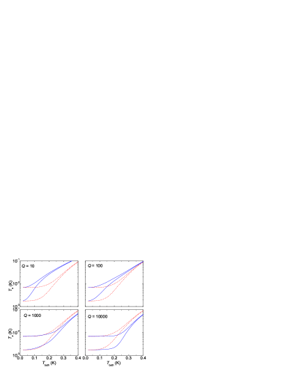
Figure 2: Minimum electron temperature in a metal wire as a function of bath temperature, cooled by SINIS tunnelling for various values of $Q$. The solid blue lines are from the one-dimensional model, and the red dashed lines from the three-dimensional model. The parameters we used correspond to Al as a superconductor and Cu as the metal wire of $L=1$ $\mu$m length; its width and thickness are assumed to be 30 nm both, $\Sigma=2\cdot 10^{9}$ WK^-5m^-3, $E=130$ GPa and $\rho=8920$ kgm^-3. The tunnel resistances of the two NIS junctions are $R_{T}=10$ k$\Omega$ both, and we assume that the non-ideality parameter of the junctions has a value $\gamma=1\cdot 10^{-4}$ (curves lying higher) or $\gamma=1\cdot 10^{-5}$ (lower).

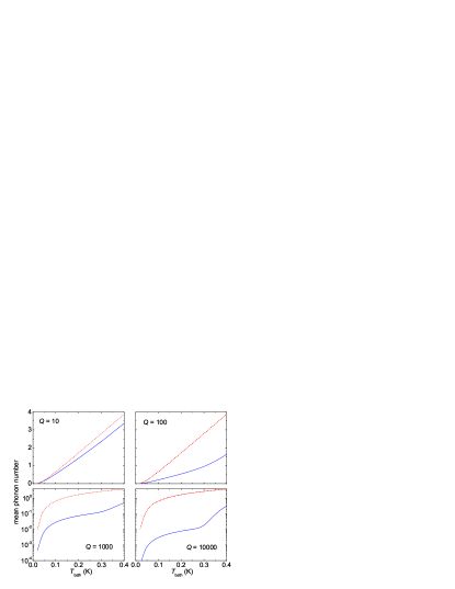
Figure 3: Population of the lowest vibrational mode in a wire against bath temperature according to the one-dimensional model. The solid (blue) lines show the population when the electron cooling is applied, whereas the dashed (red) lines are the corresponding non-cooled populations. The parameters are the same as in Fig. 2. The results for the two values of $\gamma$ are almost indistinguishable, and we have plotted only those for $\gamma=1\cdot 10^{-4}$.

We next apply the results above to determine the performance and mechanical mode cooling naik06 ; schliesser06 ; poggio07 ; brown07 in a suspended electron refrigerator. Note that overheating of a suspended wire, or a single-electron transistor li07 , can be analyzed similarly as our example of cooling below: heat currents and temperature drops are simply inverted. In a hybrid tunnel junction configuration (SINIS), with a metal island (N) and superconducting leads (S), the electron system in N can be cooled far below the bath temperature by applying a bias $eV$ of the order of the superconducting gap $\Delta$ over each tunnel junction (I) between S and N. This SINIS refrigeration technique based on energy filtering of the tunnelling electrons due to the gap in the superconductor has been applied extensively over the past decade, for a review see Ref. giazotto06 , but not yet in suspended wires to the best of our knowledge. Here we propose its use in connection with the one-dimensional phonon system. It is possible to cool not only the electrons in the wire but also the vibrational modes in it by coupling them to the cold electrons. Figure 2 shows numerically calculated results for the minimum electron temperature reached as a function of the bath temperature: at the optimum bias voltage of the junctions heat is removed from the wire at a rate $\dot{Q}\sim\Delta^{2}/(e^{2}R_{T})(T_{e}/T_{C})^{3/2}$. In steady state this heat flux is balanced by the heat flux from the phonon modes. We assume that all the relevant modes have the same quality factor $Q_{n}\equiv Q$. The collection of results in Fig. 2 shows that if $Q$ is large, strong suppression of electron temperature can be achieved. The saturation of the temperature with low $T_{\rm bath}$ is caused by the ohmic heating in the refrigerating junctions with leakage parameter $\gamma$, which has been chosen to correspond to typical experimental conditions: $\gamma$ equals the low temperature zero bias conductance of a junction normalized by the value of conductance at large voltages, and it can be conveniently included in the (normalized) density of quasiparticle states of the superconductor at energy $E$ as $n_{S}(E)=|{\rm Re}(\frac{E+i\gamma\Delta}{\sqrt{(E+i\gamma\Delta)^{2}-\Delta^{2}}})|$ giazotto06 . The cooling effect of the suspended structure differs from that of the result of the three-dimensional model; specifically the results of the one-dimensional model, valid when $w\lesssim\lambda_{\rm thermal}$, do not depend on the transverse dimensions of the wire, whereas the results of the three-dimensional model are determined by these dimensions as well via the dependence on volume in Eq. (11). Also the vibrational modes involved are cooled: this is demonstrated in Fig. 3, where we plot the population of the lowest mode, $n=1$, under the same conditions as in Fig. 2. The corresponding mode occupations in the absence of electron cooling are shown for reference. The magnitude of the mode cooling is determined by the interplay of the cooling power, electron-phonon coupling, and the coupling to the bath, determined by $Q$. From our example it seems obvious that electron-mediated cooling of the vibrational modes into the quantum limit is a feasible option, manifested by the very low mode populations, in particular when $Q$ is large.

In summary, we derived the basic relations governing electron-phonon heat transport in narrow metal wires, where the electron distribution is three-dimensional and the phonon distribution is confined to one dimension. In this realistic scenario describing suspended wires made of ordinary metals, we find that the heat currents differ drastically from those in bulk systems. In particular, we demonstrated that the vibrational modes of the wire can be cooled significantly by electron refrigeration, provided the mechanical $Q$’s of the modes are sufficiently high.

We thank the NanoSciERA project ”NanoFridge” of the EU and the Academy of Finland for financial support.

References

- (1) V. F. Gantmakher, Rep. Prog. Phys. 37, 317 (1974).
- (2) A. N. Cleland, Foundations of nanomechanics (Springer, Berlin, 2003).
- (3) K. C. Schwab and M. L. Roukes, Physics Today 58, 36 (2005).
- (4) F. Giazotto et al., Rev. Mod. Phys. 78, 217 (2006).
- (5) O.-P. Saira et al., Phys. Rev. Lett. 99, 027203 (2007).
- (6) S.-X. Qu, A. N. Cleland, and M. R. Geller, Phys. Rev. B 72, 224301 (2005).
- (7) SeGi Yu, K. W. Kim, M. A. Stroscio, and G. J. Iafrate, Phys. Rev. B 51, 4695 (1995).
- (8) T. Kühn and I. J. Maasilta, Nucl. Instrum. Methods Phys. Res. A 559, 724 (2006).
- (9) J. T. Karvonen and I. J. Maasilta, Phys. Rev. Lett., in press (2007).
- (10) T. F. Li et al., Appl. Phys. Lett. 91, 033107 (2007).
- (11) S. Rajauria et al., Phys. Rev. Lett. 99, 047004 (2007).
- (12) F. C. Wellstood, C. Urbina, and J. Clarke, Phys. Rev. B 49, 5942 (1994).
- (13) L. G. Rego and G. Kirczenow, Phys. Rev. Lett. 81, 232 (1998).
- (14) S. Sapmaz et al., Phys. Rev. Lett. 96, 026801 (2006).
- (15) see, e.g., F. Reif, Fundamentals of statistical and thermal physics (McGraw-Hill, New York, 1965).
- (16) A. Naik et al., Nature (London) 443, 193 (2006).
- (17) A. Schliesser et al., Phys. Rev. Lett. 97, 243905 (2006).
- (18) M. Poggio, C. L. Degen, H. J. Mamin, and D. Rugar, Phys. Rev. Lett. 99, 017201 (2007).
- (19) K.R. Brown et al., Phys. Rev. Lett. 99, 137205 (2007).