Field patterns in periodically modulated optical parametric amplifiers and oscillators

Abstract

Spatially localized and periodic field patterns in periodically modulated optical parametric amplifiers and oscillators are studied. In the degenerate case (equal signal and idler beams) we elaborate the systematic method of construction of the stationary localized modes in the amplifiers, study their properties and stability. We describe a method of constructing periodic solutions in optical parametric oscillators, by adjusting the form of the external driven field to the given form of either signal or pump beams.

I Introduction

Parametric amplification together with stimulated emission are fundamental mechanisms for generation of coherent radiation. Laser action is based on the latter whereas the former is the basis of optical parametric oscillations (OPOs). Even though, laser systems are encountered worldwide thanks to their intense commercialization, OPOs are, nowadays, more and more spreading (and not only in laboratories) owing, essentially, to their tunability on a wide range of frequencies. In fact, for a laser the emitted frequency is fixed once and for all to the manufacturing. In consequence, a pile of several lasers of different frequencies is needed when the operating system involves a whole range of frequencies. We thus measure the considerable advancement that OPOs bring to modern optical technology where large frequency variations are desired. Although the basic principles of optical parametric amplifiers (OPAs) have been known for over 40 years, OPOs developed quickly only in the last decade mostly for technological reasons Piskarskas . The use of periodically varying media greatly enriches the diversity of observable phenomena either in OPAs or in OPOs, allowing for existence of coherent field patterns, the study of which is the main goal of the present paper.

Compared to lasers, OPOs have received much less attention in spite of their strong interest both on the fundamental and on the technological sides Byer . We recall that these are very frequency agile coherent sources with a wide range of possible applications including range finding, pollution monitoring and tunable frequency generation. They are also the key element for the production of twin photons and the realization of fundamental quantum optics experiments Kolobov .

Basically an optical parametric amplifier (OPA) generates light via a three-wave mixing process in which a nonlinear crystal subjected to a strong radiation at frequency $\omega_{p}$ (pump beam) radiates two coherent fields at frequencies $\omega_{s}$ (signal beam) and $\omega_{i}$ (idler beam) such that the energy conservation law $\omega_{p}=\omega_{s}+\omega_{i}$ is satisfied. This energy conservation criterion may be interpreted in terms of photons where one photon at frequency $\omega_{p}$ is converted into two photons at frequencies $\omega_{s}$ and $\omega_{i}$. This process is most efficient when the phase matching condition is fulfilled. It states that optical parametric amplification is favored when the three interacting waves keep constant relative phases along their propagation inside the crystal. This implies ${\vec{k}}_{p}={\vec{k}}_{s}+{\vec{k}}_{i},$ or equivalently $n_{p}(\omega_{p})\omega_{p}=n_{s}\left(\omega_{s}\right)\omega_{s}+n_{i}\left(\omega_{i}\right)\omega_{i}$ where $\vec{k}_{j}$ and $n_{j}$ are the wavevector and the refractive index at frequency $\omega_{j}$ respectively ($j=p,s,i$).

OPOs have recently appeared as physical systems whose modeling generates specific problems sharing common grounds with very general open questions such as those related to the appearance of complexity in spatially extended systems Hohenberg . In fact, OPOs have become one of the most active fields in nonlinear optics not only for the richness in nonlinear dynamical behaviors REFSOPO but also for the potential applications of OPO devices Piskarskas , including low-noise measurements and defection Kimble ; Longhi . When driven by an intense external field, both OPAs; i.e. corresponding to a single pass through the quadratic crystal, and OPOs show a number of remarkable features among them are the localized structures (LS) or spatial solitons Firth ; Conti . These nonlinear solutions are generated in the hysteresis loop involving stable homogeneous states and the nonhomogeneous periodical branches of solutions. The latter that initiate the LS formation result from the modulational instability (often called Turing instability) and have been intensively studied in nonlinear optical cavities JOB2004 . Stability of LSs and effects of spatial inhomogeneities on the LS dynamics have been addressed in Refs. Skryabin12 ; Fedorov .

Very recently another type of LS in the form of dissipative ring-shaped solitary waves have been generated in the regime where the steady state solutions are stable with respect to the modulational instability. Indeed, it has been shown in Taki-Springer that OPOs can continuously generate spatially periodic dissipative solitons with an intrinsic wavelength. These modulations spontaneously develop from localized perturbations of the unstable homogeneous steady state that separates the two stable states of an hysteresis cycle. This constitutes the counterpart of Turing spontaneous modulations initiated by extended perturbations. They occur in the wings of the 2D traveling flat top solitons (fronts, domain walls or kink-antikink) and give eventually rise to ring-shaped propagating dissipative solitons. Such non-Turing periodic dissipative solitons have also been predicted in liquid crystal light valve nonlinear optical cavity Durniak .

In the more general context of optics the soliton ability to self-confine light beam power makes it a promising candidate for future applications in information technology Nature06 and image processing Nature02 ; Science97 . In this context, an issue of important significance is the development of a research activity aiming at taking advantage of more sophisticated geometries of cavities yulin and periodic modulations of the refractive index Conti ; All to generate, control, and stabilize optical LS. The existence of quadratic gap solitons in periodic structures, having spatial extension much bigger than the period of the structure, and thus well described within the framework of the multiple scale expansion, was studied in Conti . The control and stabilization of LS are possible since periodic transverse modulations are known, with the advent of photonic crystals, to profoundly affect spatial soliton properties All .

In this paper we address the problem of the formation and the dynamics of localized structures in presence of transverse periodic modulations of the refractive index in both OPAs and OPOs, concentrating on field patterns whose spatial scales are of order of the period of the medium. This is actually the main distinction of our statement from the previous studies exploring either slow envelope LSs Conti or the tight-binding limit leading to nonlinear lattice equations Egorov . Indeed, optical parametric wave-mixing systems are one of optical devices that can operate either as a conservative (OPAs) or a dissipative (OPOs) system. We have analytically investigated the existence and stability of conservative LS (or solitons) that appear in OPAs and the dissipative periodic patterns occurring in a parametric oscillation regime (OPOs). We have first identified the simultaneous conditions required on index modulation together with the incident pump for stationary LS to exist by means of Bloch waves approach. It results from our analysis that in a degenerate configuration (the signal and idler are identical) signal and pump fields can be found in form of phase locked LS (real solutions). They are strongly stable and located at the minimum of the index periodic modulation. To extend the analytical analysis to higher nonlinear regimes we have performed numerical simulations that allowed characterizing the different types of stable LS that can be supported by the system under transverse periodic modulations.

The paper is organized as follows. In Sec. II we briefly recall the two-wave model governing the spatio-temporal evolution of the slowly varying envelopes of the pump and the signal waves including diffraction and transverse periodic modulation of the refractive index. The general conditions required for the existence and stability of conservative LS appearing in OPAs, by means of Bloch waves approach, are given. Extension of Bloch waves approach to take into account dissipative effects stemming from cavity losses is carried out in Section III, for a degenerate OPO with transverse periodic modulations, where for construction of periodic solutions we use a kind of inverse engineering allowing us to determine the external field from a given structure of the nonlinear Bloch state. Concluding remarks are summarized in the last section.

II Localized modes in periodically modulated optical parametric amplifiers

II.1 The model

We start with the model describing optical parametric amplification where we take into account diffraction and the transverse periodic change of the refraction index ($n=n_{j}^{(0)}+n_{j}^{(1)}(\vec{r})$, $j=0,1$). In the degenerate configuration, the signal and idler fields are identical leading to the resonant frequency conversion $\omega_{0}=2\omega_{1}$ where $\omega_{0}$ and $\omega_{1}$ are the pump and signal frequencies respectively. Considering beam propagation along the $z$-direction, the nonlinear interaction of the two waves propagating in the crystal is governed by the system Tlidi :

$$\partial_{z}\alpha_{0}=\frac{i}{2}\nabla^{2}\alpha_{0}+i\tilde{\varepsilon}_{0}(\vec{r})\alpha_{0}+i\alpha_{1}^{2}e^{i\Delta kz}\,,$$ (1a)

$$\partial_{z}\alpha_{1}=i\nabla^{2}\alpha_{1}+i\tilde{\varepsilon}_{1}(\vec{r})\alpha_{1}+2i\alpha_{0}\bar{\alpha}_{1}e^{-i\Delta kz}\,,$$ (1b)

where $\alpha_{0}$, $\alpha_{1}$ are the envelopes of the pump and the idler, respectively. $\vec{r}=(x,y)$, $\nabla$ stands for the transverse gradient, and $\tilde{\varepsilon}_{j}=\omega_{j}^{2}[n_{j}^{(1)}]^{2}/c^{2}k_{j}$. Hereafter an overbar stands for the complex conjugation.

We will be interested in periodically varying refractive indexes. Let us further specify the model considering $n_{j}^{(1)}$ to be independent on frequency, i.e. assuming

$$\tilde{\varepsilon}_{0}(\vec{r})=2\tilde{\varepsilon}_{1}(\vec{r})\equiv\tilde{\varepsilon}(\vec{r}).$$ (2)

This assumption is not essential for construction of the field patterns, reported below, and is introduced only for the sake of concreteness, as the approaches we will consider involve numerical simulations. Thus, the theory developed here is straightforwardly generalized to any relation between $\tilde{\varepsilon}_{0}(\vec{r})$ and $\tilde{\varepsilon}_{1}(\vec{r})$, provided that their spatial periods coincide (as it happens in a typical experimental situation).

For perfect phase-matching, $\Delta k=0$, the system (1), (2) can be written in the Hamiltonian form $\partial_{z}\alpha_{j}=i\delta H/\delta\bar{\alpha}_{j}$ with the Hamiltonian

$$H = \int\left[-\frac{1}{2}|\nabla\alpha_{0}|^{2}-|\nabla\alpha_{1}|^{2}\right.$$ (3)

$$+ \left.\tilde{\varepsilon}\left(|\alpha_{0}|^{2}+\frac{1}{2}|\alpha_{1}|^{2}\right)+\bar{\alpha}_{0}\alpha_{1}^{2}+\alpha_{0}\bar{\alpha}_{1}^{2}\right]d^{2}\vec{r}$$

being an integral of ”motion”: $dH/dz=0$. Another integral is given by the total power $P=2P_{0}+P_{1}$, where we have introduced a notation $P_{j}=\int|a_{j}|^{2}d^{2}\vec{r}$ for the power of the $j$-th component, i.e. $dP/dz=0$. In what follows, existence domain and properties of non-uniform stationary solutions will be investigated.

II.2 General properties of stationary solutions

For the sake of simplicity, we address in the present work the situation of $y$-independent spatial patterns, i.e. we assume $n_{j}^{(1)}\equiv n_{j}^{(1)}(x)$. Without loss of generality we can impose that $n_{j}^{(1)}(x)$ is a $\pi$-periodic function (this can be always achieved by proper renormalization of the coordinate units). Then it is convenient to introduce a periodic function $V(x)\equiv-2\tilde{\varepsilon}(x)$, $V(x+\pi)=V(x)$, and to define two linear operators

$${\cal L}_{j}\equiv-\frac{d^{2}}{dx^{2}}+\frac{1}{4^{j}}V(x),\quad j=1,2$$ (4)

and the respective eigenvalue problems

$${\cal L}_{j}\varphi_{\nu q}^{(j)}(x)={\mathcal{E}}_{\nu q}^{(j)}\varphi_{\nu q}^{(j)}(x).$$ (5)

Here $\varphi_{\nu q}^{(j)}(x)$ are the linear Bloch waves, with the index $\nu=0,1,2,...$ standing for the number of the allowed band and $q$ designating the wavevector in the first Brillouin zone (BZ), $q\in[-1,1]$. In this paper we will also use the notations ${\mathcal{E}}_{\nu,\pm}^{(j)}$ for the lower (”$-$”) and the upper (”$+$”) edges of the $\nu$-th band, and $\Delta_{\nu}^{(j)}={\mathcal{E}}_{\nu+1,-}^{(j)}-{\mathcal{E}}_{\nu,+}^{(j)}$ for a $\nu$-th finite gap ($\Delta_{0}^{(j)}$ designating the semi-infinite gaps).

For a general form of $V(x)$, the introduced linear eigenvalue problems (5) represent Hill equations Hill and, as it becomes clear below, play crucial role in the systematic construction of the nonlinear localized modes (for a review see e.g. BK ).

Let us first investigate the existence of the different types of solutions of the conservative system (1), which are homogeneous in $z$-direction. Hence, we seek for non-uniform ($x$-dependent) stationary solutions of the system (1) in the form:

$$\alpha_{0}=a_{0}(x)e^{-i(k_{z}z+k_{y}y)},\quad\alpha_{1}=a_{1}(x)e^{-i(k_{z}z+k_{y}y)/2},$$ (6)

where we have taken into account the matching conditions $k_{z}=k_{z0}=2k_{z1}$, $k_{y}=k_{y0}=2k_{y1}$ and $\Delta k=0$ . Substituting the ansatz (6) in Eqs. (1) we obtain

$$\Omega a_{0}=-\frac{d^{2}a_{0}}{dx^{2}}+V(x)a_{0}-2a_{1}^{2},$$ (7a)

$$\frac{\Omega}{4}a_{1}=-\frac{d^{2}a_{1}}{dx^{2}}+\frac{1}{4}V(x)a_{1}-2a_{0}\bar{a}_{1},$$ (7b)

where $\Omega=2k_{z}-k_{y}^{2}$ is a spectral parameter of the problem.

System (7) is considered subject to the boundary conditions

$$\lim_{x\to\pm\infty}a_{0}(x)=\lim_{x\to\pm\infty}a_{1}(x)=0$$ (8)

corresponding to localized patterns in the $x$-direction.

Now we establish several general properties of the solutions. First, multiplying (7a) and (7b) respectively by $d\bar{a}_{0}/dx$ and $d\bar{a}_{1}/dx$, adding conjugated equations, and integrating over $x$ we obtain a necessary condition for existence of the localized modes:

$$\int_{-\infty}^{\infty}\frac{dV(x)}{dx}\left(2|a_{0}(x)|^{2}+|a_{1}(x)|^{2}\right)dx=0.$$ (9)

Next we notice that the Hamiltonian (3), corresponding to the effectively one-dimensional case we are interested in, can be written down in the form $H_{1D}=H_{0}+H_{V}(0)$ where

$$H_{0}=\int_{-\infty}^{\infty}\left(-\frac{1}{2}|a_{0,x}|^{2}-|a_{1,x}|^{2}+\bar{a}_{0}a_{1}^{2}+a_{0}\bar{a}_{1}^{2}\right)dx$$ (10)

is the Hamiltonian of the two-wave interactions in the homogeneous medium and

$$H_{V}(\zeta)=-\frac{1}{2}\int V(x-\zeta)\left(|a_{0}|^{2}+\frac{1}{2}|a_{1}|^{2}\right)dx$$ (11)

describes the effect of the periodicity.

Assuming that a solution $(a_{0}(x),a_{1}(x))$ of Eq. (7) is given, we consider its infinitesimal shift $\zeta$ in the space, i.e. $(a_{0}(x-\zeta),a_{1}(x-\zeta))$. For the solution to be stable, the introduced shift must lead to increase of the energy. Thus for such a solution we obtain the conditions CBKAS

$$\frac{dH_{V}(\zeta)}{d\zeta}\Bigg{|}_{\zeta=0}=0\quad\mbox{and}\quad\frac{d^{2}H_{V}(\zeta)}{d\zeta^{2}}\Bigg{|}_{\zeta=0}>0\,.$$ (12)

The first one is nothing but Eq. (9) obtained above from the energetic arguments, while the second constrain acquires specific meaning for the definite symmetry solutions and will be considered below.

II.3 On phases of the stationary localized solutions

In this section we prove that spatially localized solutions of Eqs. (7) are real. To this end, by analogy with AKS ; BK , we set $a_{j}(x)=\rho_{j}(x)e^{i\theta_{j}(x)}$, define $\theta\equiv 2\theta_{1}-\theta_{0}$, and rewrite (7) in the form

$$\rho_{0,xx}-\theta_{0,x}^{2}\rho_{0}-V_{\Omega}\rho_{0}+2\rho_{1}^{2}\cos\theta=0,$$ (13a)

$$2\theta_{0,x}\rho_{0,x}+\theta_{0,xx}\rho_{0}+2\rho_{1}^{2}\sin\theta=0,$$ (13b)

$$\rho_{1,xx}-\theta_{1,x}^{2}\rho_{1}-\frac{1}{4}V_{\Omega}\rho_{1}+2\rho_{1}\rho_{0}\cos\theta=0,$$ (13c)

$$2\theta_{1,x}\rho_{1,x}+\theta_{1,xx}\rho_{1}-2\rho_{1}\rho_{0}\sin\theta=0,$$ (13d)

where $V_{\Omega}\equiv V(x)-\Omega$. Multiplying Eq. (13d) by $\rho_{1}$ and integrating we obtain

$$\frac{d\theta_{1}(x)}{dx}=\frac{2}{\rho_{1}^{2}(x)}\int_{C}^{x}\rho_{1}^{2}(x^{\prime})\rho_{0}(x^{\prime})\sin\theta(x^{\prime})dx^{\prime}$$ (14)

where $C$ is a constant. Substituting this last formula in Eq. (13c) and considering the limit $x\to\pm\infty$ together with the boundary conditions (8) we find out that a necessary condition for the existence of nonsingular solutions is that

$$\lim_{x\to\pm\infty}\int_{C}^{x}\rho_{1}^{2}(x^{\prime})\rho_{0}(x^{\prime})\sin\theta(x^{\prime})dx^{\prime}=0.$$ (15)

Using the definition of $\rho_{j}$ and $\theta_{j}$ this constrain can be rewritten as follows

$$\lim_{x\to\pm\infty}\mbox{Im}\int_{C}^{x}\bar{a}_{0}(x^{\prime})a_{1}^{2}(x^{\prime})dx^{\prime}$$

$$=\lim_{x\to\pm\infty}\mbox{Im}\int_{C}^{x}\left(-\bar{a}_{0}(x^{\prime})\frac{d^{2}a_{0}(x^{\prime})}{dx^{\prime 2}}+V_{\Omega}(x^{\prime})|a_{0}(x^{\prime})|^{2}\right)dx^{\prime}$$

$$=\lim_{x\to\pm\infty}\mbox{Re}\left[\bar{a}_{0}(C)a_{0,x}(C)-\bar{a}_{0}(x)a_{0,x}(x)\right]$$

$$=|\rho_{0}(C)|^{2}\theta_{0,x}(C)=0$$

where we have taken into account Eq. (1a) and performed integration by parts. From the last line of the above equalities we conclude that $\theta_{0}$ does not depend on $x$, and thus without restriction of generality it can be chosen zero so that $a_{0}(x)$ can be chosen real. Then Eq. (7a) implies that $a_{1}^{2}$ is real. Thus one has two options: either $a_{1}$ is real or $a_{1}$ is pure imaginary. However, one readily concludes from the system (7) that the second option can be reduced to the first one by changing $a_{0}\mapsto-a_{0}$. Therefore, in what follows, we will restrict our analysis to real stationary fields $a_{0,1}(x)$.

II.4 Symmetry of solutions in even potentials

For the sake of concreteness and to simplify the consideration below we set $\tilde{\varepsilon}(x)$ to have a definite parity. Then recalling the second of the constrains (12) we conclude that a solution which also has a definite parity, i.e. such that $a_{j}^{2}(x)=a_{j}^{2}(-x)$, and strongly localized about $x=0$, cannot satisfy (12) if $V(x)=-V(-x)$. Moreover, for strongly localized stable solutions Eq.(12) is satisfied only if $x=0$ is a minimum of the periodic function $V(x)$. Thus we can conjecture that stable solutions will be obtained centered about the minimum of the potential.

Thus, we restrict further consideration to the case

$$V(x)=V(-x),\qquad\left.\frac{d^{2}V(x)}{dx^{2}}\right|_{x=0}>0$$ (16)

and consider $a_{0,1}$ either even or odd.

As the next step we prove that among such solutions only even are allowed, or in other words we prove the following

Proposition 1.

If $\{a_{0}(x),a_{1}(x)\}$ is a real solution of (7) with the potential (16), such that $a_{0,1}^{2}(x)=a_{0,1}^{2}(-x)$, then necessarily: $a_{0}(x)=a_{0}(-x)$ and $a_{1}(x)=a_{1}(-x)$.

Proof.

First we prove that $a_{0}(x)$ is even. Assuming the opposite, i.e. that $a_{0}(x)$ is an odd function and integrating (7a) with respect to $x$ over the whole axis we obtains $P_{1}=0$. Thus $a_{1}\equiv 0$ and (7a) becomes linear and hence does not allow for the existence of spatially localized solutions. The contradiction we have arrived to, proves the claim that $a_{0}(x)$ must be even.

Now we can prove that $a_{1}(x)$ is an even function. Again assuming that it is odd, what implies that $a_{1}(0)=0$, and designating $\displaystyle{\beta_{n}=\frac{1}{(2n+1)!}\left.\frac{d^{2n+1}a_{1}}{dx^{2n+1}}\right|_{x=0}\neq 0}$ the lowest nonzero derivative of $a_{1}(x)$ at $x=0$, such that $a_{1}(x)=\beta_{n}x^{2n+1}+o(x^{2n+1})$ as $x\to 0$, from (7a) we obtain that such a solution exists only if $V(0)-\Omega={\cal O}(x^{2})$, and consequently from (7a) $a_{0}(x)={\cal O}(x^{4(n+1)})$. Now one can estimate the orders of all terms in (7b) at $x\to 0$ as ${\cal O}(x^{2n-1})$, ${\cal O}(x^{2n+3})$, and ${\cal O}(x^{4n+1})$, i.e. (7b) cannot be satisfied in the vicinity of $x=0$. We thus again arrive at the contradiction with the supposition about the existence of the solution. ∎

II.5 On construction of spatially localized modes

Let us now turn to the asymptotics of the solutions at $|x|\to\infty$. Since in this limit, $q_{j}\to 0$, it follows directly from (7b) that $a_{1}(x)\to A_{1}(x)$ where $A_{1}(x)$ is a decaying to zero solution of the Hill equation Hill

$$-\frac{d^{2}A_{1}}{dx^{2}}+\frac{1}{4}\left(V(x)-\Omega\right)A_{1}=0.$$ (17)

This equation has decaying (growing solutions) only if $\Omega/4$ belongs to a forbidden gap of the ”potential” $\frac{1}{4}V(x)$ (here we will not consider the cases where $\Omega$ coincides with an edge of a gap). This last requirement we formulate as $\Omega/4\in\Delta_{\nu^{\prime}}^{(1)}$ for some positive integer $\nu^{\prime}$. Then it follows form the Floquet theorem that

$$A_{1}(x)=C_{1}e^{-\mu_{1}x}\phi_{1}(x)$$ (18)

where $C_{1}$ is a constant, $\mu_{1}$ is the corresponding Floquet exponent, defined by the frequency detuning to the gap, and $\phi_{1}(x)$ is the real $2\pi$–periodic function.

Let us now turn to (7a), and notice that it can be considered as a linear equation for the unknown $a_{0}(x)$. Taking into account, that for decaying solutions $a(x)$, $\Omega$ must belong to a gap $\Delta_{\nu^{\prime\prime}}^{(0)}$, of the potential $V(x)$, i.e. $\Omega\in\Delta_{\nu^{\prime\prime}}^{(0)}$ [we emphasize that the frequency $\Omega$ here is the same as in Eqs. (7b) and (17)], we arrive at a necessary condition for existence of the localized modes: there must exist a nonzero intersection between gaps $\Delta_{\nu^{\prime\prime}}^{(0)}$ and $4\Delta_{\nu^{\prime\prime}}^{(1)}$ for at least some integers $\nu^{\prime}$ and $\nu^{\prime\prime}$. Then, designating this intersection by $\Delta_{g}$, i.e. $\Delta_{g}=\Delta_{\nu^{\prime\prime}}^{(0)}\cap 4\Delta_{\nu^{\prime}}^{(1)}$ and referring to it as a total gap, we conclude that if for a given $\Omega$ a localized mode exists, then $\Omega\in\Delta_{g}$.

Now one can write down:

$$a_{0}(x) = \frac{1}{W}\left(A_{+}(x)\int_{x}^{\infty}A_{-}(x^{\prime})a_{1}^{2}(x^{\prime})dx^{\prime}+A_{-}(x)\int_{-\infty}^{x}A_{+}(x^{\prime})a_{1}^{2}(x^{\prime})dx^{\prime}\right).$$ (19)

where $A_{\pm}$ are the solutions of the eigenvalue problem

$$-\frac{d^{2}A_{\pm}}{dx^{2}}+\left(V(x)-\Omega\right)A_{\pm}=0\,,$$ (20)

and $W=A_{+}(A_{-})_{x}-(A_{+})_{x}A_{-}$ is their Wronskian. Taking into account, that $\Omega$ is in a gap of the spectrum of Eq. (20), we have that $A_{\pm}(x)=e^{\pm\mu_{0}x}\phi_{\pm}(x)$ with $\phi_{\pm}(x)$ being real $2\pi$–periodic functions, and $\mu_{0}$ being the respective Floquet exponent. Thus, in the case at hand $W=-2\mu_{0}\phi_{+}\phi_{-}+\phi_{+}(\phi_{-})_{x}-(\phi_{+})_{x}\phi_{-}$.

Using the fact that $\int_{-\infty}^{\infty}A_{+}(x)a_{1}^{2}(x)dx=0$ (this can be proved by substituting $a_{1}^{2}(x)$ from Eq.(7a) and integrating by part) the second term in (19) can be rewritten in the same integration interval as the fist one

$$a_{0}(x) = \frac{1}{W}\left(A_{+}(x)\int_{x}^{\infty}A_{-}(x^{\prime})a_{1}^{2}(x^{\prime})dx^{\prime}-A_{-}(x)\int_{x}^{\infty}A_{+}(x^{\prime})a_{1}^{2}(x^{\prime})dx^{\prime}\right).$$ (21)

II.6 Numerical study of localized modes

Now one can use the shooting method to construct localized solutions of the system (7). As the first step one has to ensure that for a chosen structure the total gap $\Delta_{g}$ exists. As the next step for a chosen $\Omega\in\Delta_{g}$, the Floquet exponents $\mu_{0,1}$ and corresponding Bloch functions $\phi_{1}$ and $\phi_{\pm}$ must be computed. Next, starting from some point $x=x_{0}$ far enough from the origin, where equation (7b) is effectively linear, one can approximate the function $a_{1}(x)$ on the interval $x_{0}<x<\infty$ by its linear asymptotics $A_{1}(x)$, which is determined by (18) with some small initial amplitude $C_{1}$. Substituting $A_{1}(x)$ into equation (21) and computing the integrals one has to obtain the value of the function $a_{0}(x_{0})$ which now can be used to find $a_{1}(x)$ at the subsequent step of the spatial grid, $x=x_{0}-dx$ by solving Eq.(7b) (we use the Runge-Kutta method). Finally, by varying the shooting parameter $C_{1}$ one has to satisfy the condition $da_{0,1}/dx=0$ at the origin $x=0$ (recall that we are looking for even solutions).

Let us now show several possible solutions of the system (7). For the numerical simulations we assume the specific form of the dielectric permittivity: $V(x)=-V_{0}\cos(2x)$. In the left panel of Fig.1 an example of the band-gap structure of Eqs. (7) with a total gap (it is indicated by the shadowed region) is shown. In this particular case this is an overlap of the first gaps of each of the equation. The profiles of the corresponding solutions for different $\Omega$ inside the total gap are shown in the right panels of Fig.1.

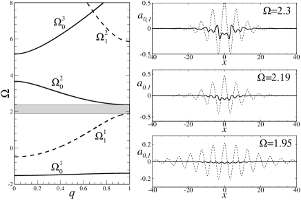
Figure 1: In the left panel the band-gap spectra $\Omega^{(\nu)}_{0}(q)$ for the pump (solid line) and $4\Omega^{(\nu)}_{1}(q)$ for the signal (dashed line) are shown. $\nu$ determines the corresponding band number. The shadowed domain shows the interval $\Delta_{g}=[1.89;2.36]$ where the first gaps for the pump and the signal have overlapping and, consequently, where localized solutions of (7) can be found. In the right panels the profiles of the localized solutions $a_{0}(x)$ (solid lines) and $a_{1}(x)$ (dashed lines) with $\Omega\in\Delta_{g}$. Here $V_{0}=4$.

In all the pictures presented one observes that the amplitude of the signal is appreciably larger than the amplitude of the pump. Moreover, the amplitude of the mode itself (it is two-component in our case) decays and the pump amplitude become very small as the frequency approaches the bottom of the total gap. Notice that the top and bottom of the total gap coincide with the top of the gap for the pump signal and with the bottom of the gap for the signal. We also observe that the pattern of the pump is more sophisticated than the pattern of the signal component.

To investigate the stability of obtained solutions we integrate numerically the evolution equations (1) taking $\Delta k=0$ and starting with initial profiles presented in the right panels of Fig. 1. In Fig. 2 we show the propagation of the localized modes for three different $\Omega$. We observe that the modes excited close to the bottom of the total gap are stable while the solutions in the vicinity of the top of the gap display unstable behavior.

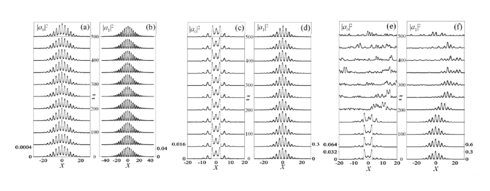
Figure 2: Dynamics of the modes, whose initial profiles are taken from the right panel of Fig. 1 and perturbed by 1% of their amplitudes. In [(a),(b)], [(c),(d)] and [(e),(f)] parameter $\Omega=1.95;2.19;2.3$, respectively.

III Coherent structures in the optical parametric oscillator

III.1 The model

Now we proceed with the study of possible coherent patterns in an optical parametric oscillator and as the first step we recall derivation of the model equations, following Tlidi . We consider the simplified case where in transverse direction there exists dependence only on one variable [we call it $x$: $\tilde{\varepsilon}\equiv\tilde{\varepsilon}(x)$] and use the abbreviated notation $\alpha_{0,1}(z,\tau)=\alpha_{0,1}(z,x,\tau)$. To this end we impose the boundary conditions on (1), (2) assuming that the cavity is located on the interval $0<z<\ell$:

$$\alpha_{0}\left(0,\tau\right) = \alpha_{0}^{in}+R_{0}e^{i\theta_{0}}\alpha_{0}(\ell,\tau-T),$$ (22a)

$$\alpha_{1}(0,\tau) = R_{1}e^{i\theta_{1}}\alpha_{1}(\ell,\tau-T)$$ (22b)

and allowing the amplitude of the driven field to depend on the transverse coordinates $x$, i.e. $\alpha^{in}\equiv\alpha^{in}(x)$. Here $T=\ell/c$ is the delay time with $c$ being the velocity of light, $\theta_{0,1}$ are the detuning parameters and $R_{0,1}$ are the reflectivity factors (in the following we will consider only the case of exact phase matching, $\Delta k=0$). In the small amplitude limit, $|\alpha_{0,1}|\ll 1$, one can write down approximated solutions for pump and signal for the reduced Maxwell equations (1) as the first order terms of the Mac-Laurin expansion

$$\alpha_{0}(\ell,\tau)=\alpha_{0}(0,\tau)+\left[\frac{i}{2}\partial_{x}^{2}\alpha_{0}(0,\tau)+i\tilde{\varepsilon}\alpha_{0}(0,\tau)+i\alpha_{1}^{2}(0,\tau)\right]\ell\,,$$ (23a)

$$\alpha_{1}(\ell,\tau)=\alpha_{1}(0,\tau)+\left[i\partial_{x}^{2}\alpha_{1}(0,\tau)+\frac{i}{2}\tilde{\varepsilon}\alpha_{1}(0,\tau)+2i\alpha_{0}(0,\tau)\bar{\alpha}_{1}(0,\tau)\right]\ell\,.$$ (23b)

Assuming that the time variation of the solutions is very slow as compared to the delay

$$T\partial_{\tau}\alpha_{0,1}(0,\tau)=\alpha_{0,1}(0,\tau+T)-\alpha_{0,1}(0,\tau)$$ (24)

and considering limits of large reflectivity $R_{0,1}\approx 1$ and small detuning $\theta_{0,1}\ll 1$ one comes to the model

$$\partial_{\tau}A_{0}=E(x)-(\gamma+i\Delta_{0})A_{0}-\frac{i}{2}{\cal L}_{0}A_{0}-A_{1}^{2},$$ (25)

$$\partial_{\tau}A_{1}=-(1+i\Delta_{1})A_{1}-i{\cal L}_{1}A_{1}+2A_{0}\bar{A}_{1}$$ (26)

(see also Refs. ZMT ; BRCTT , Refs. Conti and Egorov , where the homogeneous counterpart of this system was derived respectively withing the framework of the multiple-scale expansion for excitations with smooth envelopes and as a continuum approximation for the cavity solitons in a periodic media, originally described by the coupled discrete equations). To derive these equations one uses the renormalized fields

$$\frac{\ell}{1-R_{1}}\left(i\alpha_{0},\alpha_{1},-\frac{V(x)}{2},\frac{i\alpha_{0}^{in}}{1-R_{1}}\right)\to\left(A_{0},A_{1},\tilde{\varepsilon},E\right),$$ (27)

rescaled time and space variables:

$$\left(\frac{T}{1-R_{1}}\partial_{\tau},\frac{\ell}{1-R_{1}}\partial_{x}^{2}\right)\to\left(\partial_{\tau},\partial_{x}^{2}\right),$$ (28)

as well as the constants $\gamma=(1-R_{0})/(1-R_{1})$ and $\Delta_{0,1}=\theta_{0,1}/(R_{1}-1)$. The linear operators ${\cal L}_{0,1}$ have been defined in (4).

III.2 Nonlasing states

These states correspond to $A_{1}=0$ and thus the respective $A_{0}$ solves the stationary ($\partial_{\tau}=0$) equation

$${\cal L}_{0}A_{0}^{(st)}+2(\Delta_{0}-i\gamma)A_{0}^{(st)}+2iE(x)=0.$$ (29)

Let us consider the driven field having the same periodicity as the medium, i.e. $E(x)=E(x+\pi)$. Since the Bloch states constitute a complete orthonormal basis one can represent

$$E(x)=\sum_{\nu,q}e_{\nu q}\varphi_{\nu q}^{(0)}(x).$$ (30)

Looking for the respective stationary solution $A_{0}^{(st)}$ also in a form of the expansion over the Bloch functions one readily obtains:

$$A_{0}^{(st)}(x)=-2i\sum_{\nu,q}\frac{e_{\nu q}}{{\cal E}_{\nu q}^{(0)}+2(\Delta_{0}-i\gamma)}\varphi_{\nu q}^{(0)}(x).$$ (31)

The obtained field pattern has an interesting particular limit which occurs when $-2\Delta_{0}$ coincides with one of the band edges of the pump signal, i.e. when $-2\Delta_{0}={\cal E}_{\nu\pm}^{(0)}$. Then $A_{0}^{(st)}(x)\equiv E(x)/\gamma$, i.e. the pattern of the pump signal is the same as the pattern of the driven field (with accuracy of a factor $1/\gamma$).

III.3 Lasing states, particular case 1

In the presence of a periodic potential of a general kind, finding explicit solutions for lasing states even in the simplest statement where $A_{1}=$const seems to be an unsolvable problem. A progress however is possible for periodic functions $V(x)$ of a specific type. In order to show this we employ a kind of ”inverse engineering” BK and find an explicit form of $V(x)$ assuming that $A_{1}$ is a given complex constant: $A_{1}=\rho e^{i\varphi}$ (here both $\rho$ and $\varphi$ are real constants). Then looking for the pump filed in the form $A_{0}(x)=a_{0}(x)e^{2i\varphi}$, where $a_{0}(x)$ is a real function, we obtain from (26)

$$a_{0}(x)=\frac{1}{2}\left[1+i\Delta_{1}+\frac{i}{4}V(x)\right]$$ (32)

which after substituting in (25) yields the system of two real equations:

$$\Delta_{0} + \gamma\Delta_{1}+\frac{\gamma+2}{4}V(x)-2E_{I}=0,$$ (33)

$$\frac{d^{2}V(x)}{dx^{2}} - 2(\Delta_{0}+2\Delta_{1})V(x)-V^{2}(x)$$ (34)

$$+ 8(\gamma-\Delta_{0}\Delta_{1}+2\rho^{2}-2E_{R})=0$$

where $E_{I}=$Im$\left(Ee^{-2i\varphi}\right)$ and $E_{R}=$Re$\left(Ee^{-2i\varphi}\right)$. Eq. (34), viewed as an equation with respect to $V(x)$, can be solved in quadratures:

$$x = \int_{0}^{V}\left[\frac{2}{3}V^{3}+2(\Delta_{0}+2\Delta_{1})V^{2}-16(\gamma-\Delta_{0}\Delta_{1}+2\rho^{2}-2E_{R})V\right]^{-1/2}dV$$ (35)

where without loss of generality we have assumed that $V(x)>0$ with $V(0)=0$ and $V_{x}(0)=0$, i.e. that $x=0$ is a local minimum of the potential. This last condition implies existence of the threshold for $E_{R}$, which now must satisfy the inequality $E_{R}>(\gamma-\Delta_{0}\Delta_{1}+2\rho^{2})/2$.

The obtained expression (35) depends on many physical parameters. Therefore, to simplify the analysis, we narrow the class of the potentials considering a case example of a one-parametric family of the periodic functions $V(x)$:

$$V(x)=V_{0}(k)\mbox{sn}^{2}\left(\beta(k)x,k\right),$$ (36)

where sn$(x,k)$ is a Jacobi elliptic function with the modulus $k$, $\beta(k)=\frac{2}{\pi}K(k)$, $V_{0}(k)=6k^{2}\beta^{2}(k)$ is the potential amplitude parametrized by $k$, and $K(k)$ is a complete elliptic integral of the first kind.

We observe that in practical terms the profile described by (36) is not too sophisticate: it can be reproduced with very high accuracy by only two or three harmonics for the elliptic parameter $k$ not too close to one (see the discussion in BK ).

Assuming that the refractive index of the cavity has the profile (36), one finds that in order to support the stationary modes one has to apply the following form of the driven filed

$$E(x)=e^{2i\varphi}\left[E_{R}+iE_{I0}+iE_{I1}\mbox{sn}^{2}(\beta x,k)\right]$$ (37)

where $E_{I0}=(\Delta_{0}+\gamma\Delta_{1})/2$ and $E_{I1}=-(\gamma+2)V_{0}(k)/8$ are fixed by the periodic structure and the cavity properties, while $E_{R}$ is the control parameter which can be changed. Then the field pattern is obtained from (32):

$$\rho^{2}=-\frac{3}{4}k^{2}\beta^{4}(k)-\frac{1}{2}(\gamma-\Delta_{0}\Delta_{1})+E_{R},$$ (38)

$$a_{0}(x)=\frac{1}{2}\left[1+i\Delta_{1}+\frac{i}{4}V_{0}\mbox{sn}^{2}(\beta(k)x,k)\right].$$ (39)

provided the elliptic modulus $k$ is expressed in terms of the detunings $\Delta_{0,1}$ through the implicit equation

$$(1+k^{2})\beta^{2}(k)=-\Delta_{1}-\Delta_{0}/2.$$ (40)

The last equation means that $V_{0}$ and $\Delta_{0,1}$ are not independent parameters and have to be matched and that the solutions we are dealing with exists only if at least one detuning is negative, or more precisely if $2\Delta_{1}+\Delta_{0}<0$.

Now, taking into account that $\rho$ is a real constant one comes to the following threshold value $E_{thr}$ for the control parameter $E_{R}$

$$E_{R}>E_{thr}=\frac{3}{4}k^{2}\beta^{4}(k)+\frac{1}{2}(\gamma-\Delta_{0}\Delta_{1}).$$ (41)

As it is clear $E_{thr}$ corresponds to $\rho=0$. In Fig.3 the dependence of the critical value of the driven field $E_{thr}$ on the depth of modulation of the refractive index, $V_{0}$, is shown.

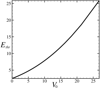
Figure 3: The dependence $E_{thr}$ vs $V_{0}(k)$ for $\gamma=1$ and $\Delta_{1}=1$.

In Fig.4 we show several patterns for different values of the amplitude of modulation of the refractive index, $V_{0}$, and of the control parameter, $E_{R}$. Using initial dynamical equations (25), (26) we have checked that all the solutions presented are dynamically stable against initial small (of order of 5% of the intensity) perturbations.

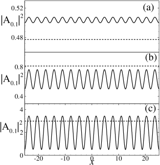
Figure 4: Patterns of the pump $|A_{0}|^{2}$ (solid line) and signal $|A_{1}|^{2}$ (dashed line) waves determined by (38), (39) for different $V_{0}$ and $E_{R}$. In (a) $V_{0}=0.06$, $E_{R}=3$, $\Delta_{0}=-4.03$, in (b) $V_{0}=1.73$, $E_{R}=4$, $\Delta_{0}=-4.88$. in (c) $V_{0}=10.24$, $E_{R}=11$, $\Delta_{0}=-9.63$. The other parameters are $\gamma=1$ and $\Delta_{1}=1$.

III.4 Lasing states, particular case 2

The approach, based on the inverse engineering and described in Sec. III.3, can be generalized. Indeed, let us look for a plane wave solution of the form

$$A_{0}=\left[\frac{1}{2}+i\tilde{A}_{0}(x)\right]e^{-2i\omega\tau},\quad A_{1}=\tilde{A}_{1}(x)e^{-i\omega\tau}$$ (42)

where $\omega$ is a frequency to be determined and $\tilde{A}_{0,1}(x)$ are real functions depending only on $x$ (c.f. (32) where $\tilde{A}_{0}=\Delta_{1}/2+V(x)/4$). Here we use the form of the potential as in the Sec.II F, namely $V(x)=-V_{0}\cos(2x)$.

Let us now require $\tilde{A}_{0}$ to be a Bloch state of the linear eigenvalue problem

$$\frac{1}{2}{\cal L}_{0}\tilde{A}_{0}+\Delta_{0}\tilde{A}_{0}=2\omega\tilde{A}_{0}\,.$$ (43)

As it is clear $2\omega$ must be a frequency bordering a gap, i.e. there must be $\omega=\frac{1}{4}{\cal E}_{\nu\pm}^{(0)}+\frac{1}{2}\Delta_{0}$, since otherwise the eigenvalue $\tilde{A}_{0}$ is complex. The amplitude of $\tilde{A}_{0}(x)$ is a free parameter, so far, because (43) is linear. Let us now fix it by requiring the frequency $\omega$ to border a gap of another linear eigenvalue problem, which reads

$$\left[{\cal L}_{1}-2\tilde{A}_{0}(x)\right]\tilde{A}_{1}+\Delta_{1}\tilde{A}_{1}=\omega\tilde{A}_{1}\,.$$ (44)

Then $\tilde{A}_{1}$ is a Bloch state of this new problem where the effective periodic potential is given by $\tilde{V}(x)=V(x)/4-2\tilde{A}_{0}(x)$. Designating the gap edges of the Hill operator (44) by $\tilde{\cal E}_{\nu\pm}^{(1)}$ (notice that they depend on the amplitude of $\tilde{A}_{0}(x)$), we deduce that the amplitude of the pump signal $\tilde{A}_{0}(x)$ is determined from the relation

$$\tilde{\cal E}_{\nu\pm}^{(1)}+\Delta_{1}=\frac{1}{4}{\cal E}_{\nu\pm}^{(0)}+\frac{1}{2}\Delta_{0}\,,$$ (45)

which can be solved numerically. The system (25), (26) is satisfied if the complex field is chosen in the form

$$E(x) = \left[\frac{\gamma}{2}+\tilde{A}_{1}^{2}(x)+i\left(\frac{1}{4}V(x)-\omega+\frac{1}{2}\Delta_{0}+\gamma\tilde{A}_{0}(x)\right)\right]e^{-2i\omega\tau}.$$ (46)

In Fig.5 we illustrate a band structure of (44) (panel a) as well as effective potential $\tilde{V}(x)$ (panel b) with $\tilde{A}_{0}(x)$ taken at the band edge ${\cal E}_{0+}^{(0)}$ and having the amplitude $1$. The patterns of $\tilde{A}_{1}(x)$ corresponding to the three lowest band edges denoted as A, B and C and the respective profiles of driving field $|E(x)|^{2}$ are shown in Fig. 5 (c)-(h).

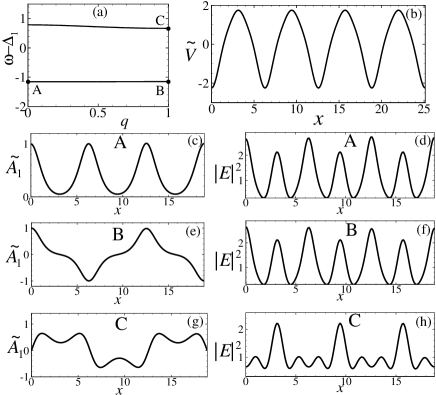
Figure 5: In (a) the band structure of the linear eigenvalue problem (44) and in (b) the profile of the corresponding effective potential, $\tilde{V}(x)$, are shown. In [(c),(d)], [(e),(f)], and [(g),(h)] the solutions, $\tilde{A}_{1}(x)$, corresponding to the first three edges of the bands denoted by points A (the edge ${\cal E}^{(1)}_{0-}$), B (the edge ${\cal E}^{(1)}_{0+}$), and C (the edge ${\cal E}^{(1)}_{1-}$) as well as corresponding profiles of the intensity of the driving field $|E(x)|^{2}$ calculated from (46) are shown. The profile of $\tilde{A}_{0}(x)$ is calculated at the upper edge of the first band ${\cal E}^{(0)}_{0+}$ of the linear eigenvalue problem (43). The other parameters are $\gamma=1$ and $V_{0}=1$.

IV Concluding remarks

In this paper we have carried out analytical and numerical studies of localized modes in optical parametric amplifiers and of periodic patterns in parametric oscillators generated by a properly chosen driving field in presence of diffraction and transverse periodic modulations of the refractive index.

Using Bloch waves approach we have found that the presence of refractive index modulations drastically affect the existence and properties of localized structures in the both systems. In particular, spatial modulations lead to the formation of transverse phase locked (real fields) signal and pump in the form of a localized modes (gap solitons). Conditions required on the amplitude of modulations and external pump field for the existence of localized patterns in the parametric oscillators have been deduced. We have checked the stability of the obtained solution by means of integration of respective dynamical equations. It as to be emphasized however that the thorough analysis of the stability of gap solitons, which is complicated by the necessity of numerical generation of exact gap solitons, is left for further studies. In the present work we also did not discuss gap solitons of high order gaps, whose existence is strongly constrained (and may be even inhibited) by the necessity of the overlapping of the spectra of two components, i.e. of the first and second harmonics (notice that the respective constrains do not exist in the theory of the single-component solitons in Kerr media). And meantime, the method elaborated for the particular case, where signal and idle waves were equal, allows straightforward generalization to the situation where resonant interaction among three different waves occurs.

- (1) See e.g. A. P. Piskarskas, Opt. Photon. News, July 1997, 25; and R. L. Byer and A. P. Piskarskas, feature issue on optical parametric oscillators, J. Opt. Soc. Am. B10, 1655 (1993).
- (2) R. L. Byer, Optical parametric oscillators in Quantum Electronics, H. Rabin and C. L. Tang eds. (Academic, New York 1975).
- (3) M. I. Kolobov, Quantum Imaging, Springer, NY, 2007.
- (4) M. C. Cross and P. C. Hohenberg, Rev. Mod. Phys. 65, 851 (1993).
- (5) K. Staliunas, Opt. Comm. 91, 82 (1992); J. Mod. Opt. 42, 1261 (1995); G.-L. Oppo, M. Brambilla, and L. A. Lugiato, Phys. Rev. A 49, 2028 (1994); G. J. de Varcarcel, K. Staliunas, E. Roldan, and V. J. Sanchez-Morcello, Phys. Rev. A 54, 1069 (1996); 56, 3237 (1997).
- (6) S. Longhi, Phys. Rev. A 53, 4488 (1996)
- (7) H. J. Kimble, Fundamental systems in quantum optics (J. Dalibard, J. M. Raimond, J. Zinn-Justine, Elsevier Sc., Amsterdam), 545 (1992).
- (8) D. V. Skryabin and W. J. Firth, Opt. Lett. 24, 1056 (1999).
- (9) C. Conti, G. Assanto, and S. Trillo, Opt. Exp. 3, 389 (1998).
- (10) P. Mandel and M. Tlidi, J. Opt. B: Quantum Semiclass. Opt. 6, R60 (2004).
- (11) D. V. Skryabin, Phys. Rev. E 60, 3508(R) (1999).
- (12) S. Fedorov, D. Michaelis, U. Peschel, C. Etrich, D. V. Skryabin, N. Rosanov, and F. Lederer, Phys. Rev. E 64, 036610 (2001).
- (13) S. Coulibaly, C. Durniak, and M. Taki, Spatial dissipative solitons under convective and absolute instabilities in optical parametric oscillators, to be published in Springer 2007, Nail Akhmediev Ed.
- (14) C. Durniak, M. Taki, M. Tlidi, P. L. Ramazza, U. Bortolozzo, and G. Kozyreff, Phys. Rev. E 72, 026607 (2005); M. Taki, M. San Miguel, and M. Santagiustina, Phys. Rev. E 61, 2133 (2000).
- (15) Spatial solitons under control, Nature Physics, vol. 2(3), Nov. (2006).
- (16) S. Barland, J. R. Tredicce, M. Brambilla, L. A. Lugiato, S. Balle, M. Guidici, T. Maggipinto, L. Spinelli, G. Tissoni, T. Knödl, M. Miller, and R. Jäger, Nature 419, 699 (2002).
- (17) A. W. Snyder and D. J. Mitchell, Science 276, 1538 (1997).
- (18) A.V. Yulin, D. V. Skryabin, P. St. J. Russell, Opt. Exp. 13, 3529 (2005).
- (19) A. G. Vladimirov, D. V. Skryabin, G. Kozyreff, P.Mandel, and M. Tlidi, Opt. Exp. 14,1 (2006) and references therein; Y. V. Kartashov, A. A. Egorov, L. Torner, and D. N. Christodoulides, Opt. Lett. 29, 1918 (2004); D. Gomila, R. Zambrini, G.-L. Oppo, Phys. Rev. Lett. 92, 053901 (2004); D. Gomila, G.-L. Oppo, Phys. Rev. E 72, 016614 (2005).
- (20) O. Egorov, U. Peschel, and F. Lederer, Phys. Rev. E 72, 066603 (2005).
- (21) M. Tlidi, M. Le Berre, E. Ressayre, T. Tallet, and L. Di Menza, Phys. Rev. A 61, 043806 (2000).
- (22) W. Magnus and S. Winkler, Hill’s Equation (Dover Publications, INC. New York, 1966).
- (23) V. A. Brazhnyi and V. V. Konotop, Mod. Phys. Lett. B 18, 627 (2004).
- (24) H. A. Cruz, V. A. Brazhnyi, V. V. Konotop, G. L. Alfimov, and M. Salerno, Phys. Rev. A 76, 013603 (2007); cond-mat/0702330.
- (25) G. L. Alfimov, V.V. Konotop, and M. Salerno, Europhys. Lett. 58, 7 (2002).
- (26) M. Le Berre, E. Ressayare, S. Coulibaly, M. Taki, and M. Tlidi (unpublished).
- (27) R. Zambrini, M. San Miguel, C. Durniak, M. Taki, Phys. Rev. E 72, 025603(R) (2005).