Adapted Downhill Simplex Method for Pricing Convertible Bonds

Abstract.

The paper is devoted to modeling optimal exercise strategies of the behavior of investors and issuers working with convertible bonds. This implies solution of the problems of stock price modeling, payoff computation and min-max optimization.

Stock prices (underlying asset) were modeled under the assumption of the geometric Brownian motion of their values. The Monte Carlo method was used for calculating the real payoff which is the objective function. The min-max optimization problem was solved using the derivative-free Downhill Simplex method.

The performed numerical experiments allowed to formulate recommendations for the choice of appropriate size of the initial simplex in the Downhill Simplex Method, the number of generated trajectories of underlying asset, the size of the problem and initial trajectories of the behavior of investors and issuers.

1. Introduction and Problem Formulation

1.1. Convertible Bonds

One type of securities at modern financial market is a convertible bond. They belong to most popular securities of modern financial market. This type of securities is of interest for both small developing companies for attracting investments and for investors, since for the latter such bonds are highly profitable.

Strategies of the behavior of investors and issuers for early exercise decision must be chosen in such a way that the issuers’ payoff will be minimal while the investors’ profit will be maximal.

A standard convertible bond is a bond that gives the holder (investor) the right to exchange (convert) it into a predetermined number of stock during a certain, predetermined period of time [ref1].

Convertible bonds are characterized by the following options:

The Issuers Options

• Call price $K_{t}$

  This option allows the issuer to call back the convertible bond at the time $t$ with the payment $K_{t}$ to the investor.

• Call Notice Period $time_{notice}$

  Before calling back the convertible bond the issuer announces his intend and can call convertible bond only after the call notice period $time_{notice}$. During this period the investor may convert the bond (”force conversion”).

The Investors Options

• Number of stocks $n$

  The investor may convert the bond into $n$ stocks at any time during the predetermined period.

• Put price $P_{t}$

  This option allows the investor to sell the convertible bond at the price $P_{t}$ during the predetermined period.

Common Options of Convertible Bonds and Stocks

• Maturity Time $T$

  The expiry time of a convertible bond.

• Face Value of Convertible Bond $N$

  The predetermined price of a convertible bond which the issuer will pay to the investor at maturity time.

• Redemption Ratio $\kappa$

  This is a preset percentage of the face value of a convertible bond which increases the price of the face value. So, the $\kappa N$ instead of $N$ may be paid by the issuer to the investor. Usually $\kappa$ is equal to 1.

• Price of Coupon Bond $B_{t}$

  This is the premium paid by the issuer to the investor at some fixed time moments during the preset period.

• Value of continuation $V_{t}$

  This is the price of a convertible bond at every time moment during the period when this convertible bond is alive. $V_{t}$ is valued by the amount of money which the owner may get by converting the bond into stocks.

• Current Stock price $S_{t}$

  This is the current price of stocks owned by the issuer.

• One Option

  The issuer or investor can perform only one action with the convertible bond, i.e. if the investor converts the bond the latter expires, as well as if the issuer wants to call the bond this cannot be stopped.

Finally, the initial conditions at the time $t=0$ are:

• $K_{t}>N$

  The call price of a convertible bond is greater than its face value.

• $P_{t}<N$

  The put price of a convertible is less than its face value.

• $n=N/(S_{0}\cdot\eta)$, where $\eta>1$.

  $n$ is the number of stocks obtained by conversion of a bond. This value is calculated under assumption that the stock price at the initial moment is greater than the real one.

1.2. Problem Formulation

Objective function is as a payoff gained by the investor. This means that the payoff is a nonnegative number.  It is clear that the investor wants to maximize the payoff, while the the issuer wants to minimize it. This payoff is based on the behaviors of the investor and the issuer and on current stock price at the time $t$.
The problem under consideration is to find such strategies for the investor $Conv_{t}$ and the issuer $Call_{t}$ which maximize the investor’s payoff and minimize the payoff payed by the issuer to investor, simultaneously. In other words, we have a min-max optimization problem for computing the issuer’s and investor’s strategies.

(1) $$\max_{Conv_{t}}\min_{Call_{t}}\textbf{payoff}(Conv_{t},Call_{t})$$

The natural choice of the boundary conditions for the investor’s and issuer’s strategies is the following:

(2) $$Conv_{t}\geq N$$

(3) $$K_{t}\geq Call_{t}\geq N$$

We consider (3) only under the condition $T-t>time_{notice}$ because otherwise the investor will not have enough time to realize his right to call back a convertible bond.
 Additionally, we introduce some initial settings, where we assume that we have a zero coupon convertible bond (no coupon payment during the preset period is done: $B_{t}=0$).

Also, we use the following preset parameters:

  $N=constant$      $\kappa$ = 1      $(K_{t}=constant)$ and $(K_{t}>N)$      $S_{0}=constant$. ($S_{0}\cdot n<N$)      $\eta>1$, say $\eta=1.1$      $n=N/(S_{0}\cdot\eta)$      Initial Guess: $Conv_{t}=K_{t}+\varepsilon$; $Call_{t}=N+\varepsilon$      $time_{notice}=const$

The maximization problem (1) - (4) will be solved by the global Downhill Simplex method, see [ref3] and stock prices are modeled by Monte Carlo simulations presented in [ref2].

The fact that such a problem can be solved numerically using this approach was shown in the Master Thesis [ref25].

Section 2 of this paper is devoted to the description of the methods for stock price generating, payoff computation, approximations of the strategy of the behaviors of the investor and the issuer, as well as the description of the Downhill Simplex method.

In Section 3 we present the results of the numerical experiments with model under consideration. In these experiments we try to determine the best values for such input parameters as size of the simplex in Downhill Simplex method, the best choice for the initial trajectories, the optimal of trajectories used for the stock price generation and the appropriate number of the points for trajectories approximations.

We finalize our work by making conclusions and giving some guidelines for further investigation in Section 4.

2. Numerical Issues

2.1. Stock Price Generating

The first step in solving the problem (1)-(3) is to generate stock prices. This can be done by different methods, and we base our computation on the method producing the Brownian motion type trajectories (see e.g. [ref2]). This method generates trajectories without jumps.
The initial stock price $S_{0}$ is given. The formula for generating the stock price without jumps at $t+1$ time moment is:

(4) $$S_{t+1}=S_{t}\cdot e^{(r-\delta-\sigma^{2}/2)\cdot\triangle+\sigma\cdot\sqrt{\triangle}\cdot Z_{t+1}}$$

where $S_{t}$ is the stock price at the current time moment $t$; $r$ is the interest rate; $\delta$ is the dividend yield of the issuer stocks (underlying asset); $\sigma$ is the volatility; $\triangle=\frac{1}{250}$ is the time step at 250 working days a year and $\{Z_{t+1},t\geq 0\}$ is a sequence of independent standard normal random variables.

2.2. Computation of the Payoff

We use the Monte Carlo method for modeling a real payoff. For this purpose we generate M, a large number of trajectories, of the issuer stock prices according to (4), and then compute $payoff_{i}$ for each of them according to Algorithm 1.

Algorithm 1 Payoff (objective function) Computation

  

  $payoff=0$

  $flag_{notice}=0$

  $time_{check}=0$

  

  for $t=0:T$ $(T=maturity\cdot 250)$ do

     

     if $S_{t}>Conv_{t}$ then

        $payoff=S_{t}$ (conversion or force conversion during the notice period)

        $break$

     end if

     if $flag_{notice}=1$ then

        if $time_{check}=time_{notice}$ then

           $payoff=K_{t}$ (call)

           $break$

        else

           $time_{check}=time_{check}+1$

        end if

     else

        if $(S_{t}>Call_{t})$ and $((T-t)>time_{notice})$ then

           $flag_{notice}=1$ (start call notice period)

        end if

     end if

     if $t=T$ then

        $payoff=N$ (the face value)

     end if

  end for

The put price $P_{t}$ is less than the face value $N$. In the case of maximization of the investor’s payoff we will not take into account $P_{t}$ and suppose that the investor does not use the possibility of choosing the put option.

Finally, the real payoff is:

(5) $$payoff=\frac{1}{M}\cdot\sum_{i=1}^{M}payoff_{i}$$

In this study we simplify the problem by setting $r=const$; $\delta=const$ and $\sigma=const$.

2.3. Optimization procedure by Downhill Simplex Method

As we solve a min-max optimization problem (1), the optimization procedure is to be applied twice at each iteration: once as a maximizer of the objective w.r.t. the investor’s strategy and then as a minimizer w.r.t. the issuer’s strategy.

In other words, we find a pair of trajectories $(Conv_{t}^{*},{Call_{t}}_{*})$ which satisfy the conditions:

(6) $$\text{payoff}(Conv_{t}^{*},Call_{t})=\max_{Conv_{t}}\textbf{payoff}(Conv_{t},Call_{t})$$

(7) $$\text{payoff}(Conv_{t}^{*},{Call_{t}}_{*})=\min_{Call_{t}}\textbf{payoff}(Conv_{t}^{*},Call_{t})$$

The optimization problem under consideration is very computational expensive due to the Monte Carlo simulations used of evaluation of the objective function, thus we do not apply the optimization methods based on derivatives computation.

To perform the optimization procedure in the most efficient way we use a derivative-free Downhill Simplex method [ref3], which is also easy implementable.

Below we give a description of this algorithm for minimizing some function $f(x)$.

Firstly we need to specify the initial $m+1$ dimensional simplex by taking $m$ points around the initial guess $x^{1}$. The point with the highest function value $f_{max}$ is called $x_{max}$.

The main idea of the Downhill Simplex method is to substitute a point with the coordinates $x_{max}$ by another point with better function value (e.g. get lower $f_{max}$ in case of minimization problem). This is done by means of Reflection, Expansion, Contraction and Multiple Contraction. Let consider these functions shortly.

Firstly, we introduce the point $x_{center}$ (the center point of the simplex for current iteration):

(8) $$x_{center}=\frac{1}{m+1}\sum_{i=1}^{m+1}{x^{i}}$$

• Reflection

  The point $x_{max}$ is reflected into $x_{max}^{*}$ so that it lies on the opposite (to the point $x_{max}$) side of the line containing $x_{max}$ and $x_{center}$. The distance between $x_{center}$ and $x_{max}^{*}$ depends on a positive constant $\alpha$ - reflection coefficient and is computed as

  (9) $$x_{max}^{*}=(1+\alpha)\cdot x_{center}-\alpha\cdot x_{max}$$

• Expansion

  The expansion process is a prolongation of Reflection, and the new point $x_{max}^{**}$ is found as:

  (10) $$x_{max}^{**}=\gamma\cdot x_{max}^{*}+(1-\gamma)\cdot x_{center}$$

  where $\gamma(\gamma>1)$ is the expansion coefficient.

• Contraction

  The contraction process puts the next point between $x_{max}$ and $x_{center}$, and the new point $x_{max}^{*}$ can be found as:

  (11) $$x_{max}^{*}=\beta\cdot x_{max}+(1-\beta)\cdot x_{center}$$

  where $0<\beta<1$ is the contraction coefficient;

• Multiple Contraction

  Here all the points are shifted according to the following rule:

  (12) $$x^{i}=(x^{i}+x_{min})/2,\ i=1,..m+1$$

  where $i$ is the number of points in the simplex and $x_{min}$ corresponds to the point with the minimal function value $f_{min}$.

In Algorithm 2 we implement the Downhill Simplex method described in [ref4].

Algorithm 2 Downhill Simplex Method

  Choose the initial guess $x^{1}$

  Choose the size of initial simplex $k$

  Choose the maximum number of iterations $max_{iter}$

  Choose the termination criterion $\epsilon$

  

  for $i=2:m+1$ do

     $x^{i}=x^{1}$

     $x_{i}^{i}=x_{i-1}^{i}+k$

     $f(i)\equiv f(x^{i})$

  end for

  MAIN LOOP

  for $i=1:max_{iter}$ do

     Find $f_{max}$, $f_{min}$, and $f_{nearest_{max}}$

     

     if (($i==max_{iter}$) or ($(f_{max}-f{min})<\epsilon$)) then

        $break$

     end if

     

     Reflection $x_{max}$ to $x_{max}^{*}$, and find $f_{max}^{*}$

     

     if $f_{max}^{*}<f_{min}$ then

        Expansion $x_{max}^{*}$ to $x_{max}^{**}$ and find the new function value $f_{max}^{**}$

        

        if $f_{max}^{**}<f{max}^{*}$ then

           $f_{max}^{*}=f_{max}^{**}$, $x_{max}^{*}=x_{max}^{**}$

        end if

     else

        if $f_{max}^{*}>f_{nearest_{max}}$ then

           Contraction $x_{max}$ to $x_{max}^{*}$, and find $f_{max}^{*}$

           

        end if

     end if

     

     if $f_{max}^{*}>f_{max}$ then

        Multiple Contraction

     else

        $x_{max}=x_{max}^{*}$, $f_{max}=f_{max}^{*}$

     end if

  end for

We denote as $x^{i}$ the whole strategy on $i$th iteration consisting of all $j$ points and $x_{j}$ is the $j$ component of the strategy $x^{i}$.

So, for solving the maximization problem (6) we use the Algorithm 2, where we minimize the objective function $-f$. The problem (7) is solved by Algorithm 2 directly.

2.4. Dimension of the Problem and Investor(Issuer) Trajectory Approximation

The trajectories $Conv_{t}$ and $Call_{t}$ are the vectors of length $250\cdot Maturity$ and $250\cdot Maturity-CallNoticePeriod$, respectively. Since the lengthes of these vectors are the dimension of the optimization problem, it is clear that such a problem cannot be solved efficiently by any optimization method. In order to reduce the dimension of the problem, solved by the Downhill Simplex Method we shall consider some approximations of the trajectories instead of the original extremely costly computable trajectories.

So, instead of considering whole trajectories $Conv_{t}$ and $Call_{t}$ in optimization procedure described above, we use a set of threshold points $x_{i}$- the critical dates from the first possible exercise date till last exercise date at maturity $T$. The trajectories are approximated by piecewise linear functions with nodes being the threshold points $x_{i}$.

We will use $5-15$ points approximation of the trajectories which means that the optimization problem will be $5-15$ dimensional, too.

Since we have a Brownian type modeling, the deviations of the prices from the initial state will increase while approaching the maturity. This is also natural for any market that the most interesting and important actions take place at the end. So, the distributions of the points should meet this requirement. According to [ref25] we consider the following distribution of the threshold points:

(13) $$x_{i+1}=\frac{x_{m}-x_{i}}{2}+x_{i},\ i=1,..m-2$$

where $x_{1}=0$ and $x_{m}=T$ or $x_{m}=T-time_{notice}-1$ for the investor’s and issuer’s trajectories accordingly. Also $m$ is the number of points in approximation.
Note that for the investor’s trajectory the function value at the point $x_{m}=T$ is always equal to $N$.

2.5. Short Description of the Main Algorithm

As a termination criterion we use the value of the gap. The gap is the difference between the investors and issuers payoff. For each iteration it is defined as:

(14) $$\text{gap}=\text{payoff}(Conv_{t}^{*},Call_{t})-\text{payoff}(Conv_{t}^{*},{Call_{t}}_{*})$$

where $payoff(Conv_{t}^{*},{Call_{t}})$ and $payoff(Conv_{t}^{*},{Call_{t}}_{*})$ are the optimizers for the problems (6)- (7) respectively.

From the optimization point of view, due to the definition (14), the gap is always nonnegative.

The main algorithm for solution the problem (1) - (4) is sketched in the Algorithm 3.

Algorithm 3 Body of the main loop

  

  $gap=gap_{old}=10$

  while (($gap>\epsilon$) and ($gap_{old}>\epsilon$)) do

     $gap_{old}=gap$

     compute $payoff(Conv_{t}^{*},{Call_{t}})$ from (6) by one step of Algorithm 2

     compute $payoff(Conv_{t}^{*},{Call_{t}}_{*})$ from (7) by one step of Algorithm 2

     $gap=payoff(Conv_{t}^{*},{Call_{t}})-payoff(Conv_{t}^{*},{Call_{t}}_{*})$

  end while

where $\epsilon$ is a small constant, say $\epsilon=0.0001$.

3. Numerical Results

The numerical model described above has a quite complicate structure and is sensitive to the choice of the input parameters. In this section we investigate the dependence of the performance of the method on some of parameters. This analysis is used to validate the numerical model and choose the parameters which give a reasonable and fast solution.

In each experiment we compute and compare the optimal strategies of the investor and the issuer. Moreover, we present the history of the behavior of the optimal value of the objective, i.e. the investor’s payoff.

While comparing the results of the numerical experiments with different initial parameters it is necessary to assume that due to the specificity of the given optimization problem the following conditions are to be fulfilled:

• The strategies of the issuer and the investor must change their behavior near the maturity time, see Section 2.4;

• The objective function must produce dumping oscillations due to the nature of the $min-max$ problem.

Below we present the experiments where 4 parameters (initial conditions) of the optimization problem are varied. These parameters are: the number of generated trajectories, the size of the simplex, the initial guess and the number of points for approximation strategies of the investor and the issuer (the size of the problem).

In each experiment the optimization problem is solved 3 times for 3 experimental values for each of the four parameters, three other parameters being fixed (are from the basic set).

The basic set of the parameters is the following:

(15) number of generated trajectories M $$= 525$$

(16) size of simplex k $$= 3$$

(17) size of the problem m $$= 10$$

(18) $$\text{initial guess}\ \varepsilon = 5$$

The rest of the parameters of the problem are constant values, such as:

• Initial Stock Price = $98;

• Convertible Bond Price (Face value) = $100;

• Call Price = $110;

• Call Notice Period = 10 days;

• Interest Rate = 0.05 (5%);

• Dividend yield = 0.1;

• Volatility = 0.2 (20%);

• Maturity = 2 (two years).

3.1. Experiment 1: Different number of trajectories for Stock Price generating

Presented here are the results for 3 different sets of generated trajectories: $M=50,525$ and $1000$. The rest of the parameters are (16) - (18).

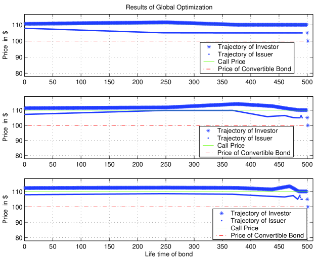
Figure 1. Strategies of Investor and Issuer. Different number of trajectories

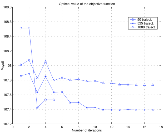
Figure 2. Objective function history. Different number of trajectories

Analyzing the above figures, one can see that the solution corresponding to the case with 50 trajectories cannot be considered to be proper as the number of trajectories is insufficient. Firstly, subplot 1 in Figure 1 shows that the behavior of the strategies close to the maturity does not change. This means that the amount of generated strategies has no real affect on the strategies of the investor and the issuer at the end of the bond lifetime. Secondly, Figure 2 shows that the method terminates rather fast, which is not appropriate for this min-max problem.

The behavior of the investor’s and the issuer’s optimal strategies as well as the objective function history are similar in the cases with 525 and 1000 trajectories (see Figure 2 and subplots 2-3, Figure 1). Thus, these numbers of generated stock price trajectories can be accepted for future experiments.  In the basic set (15) - (18) we consider 525 trajectories since the time needed for function evaluation for this case is much shorter than the one for the case with 1000 trajectories, but the solution is acceptable thereat.

3.2. Experiment 2: Different sizes of simplex

This experiments concerns the proper choice of the parameter $k$, which is the distance between the neighbor nodes in the initial simplex used in Downhill Simplex method. This experiment we run for 3 sizes of the initial simplex: $k=1,3$ and $5$. The rest of the parameters are (15) and (17)- (18).

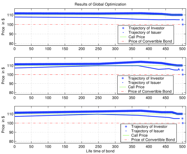
Figure 3. Strategies of Investor and Issuer. Different sizes of initial simplex

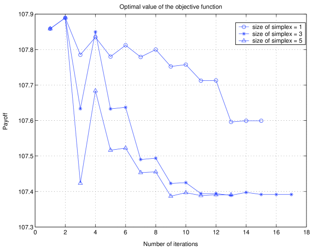
Figure 4. Objective function history. Different sizes of initial simplex

Figure 4 shows that for the minimal size of simplex $k=1$ we have oscillation with small amplitude. So, the behavior of strategies of the investor and the issuer do not change essentially w.r.t the initial guess (see subplot 1, Figure 3).

On the contrary, for maximal size of simplex $k=5$, the first solution of the minimization has a dominating effect. In other words, the first step down (the solution of the minimization problem) has a big magnitude, which does not allow to produce sufficiently big second step up (the solution of the maximization problem). This effect manifests itself in subplot3, Figure 3, where the functions corresponding to the strategies of the investor and the issuer are flat near the maturity time.

So, we choose the size of simplex $k=3$, which produces reasonable steps for both strategies (see subplot 2, Figure 3).

3.3. Experiment 3: Different initial trajectories

For any global optimization procedure the initial guess, which is the initial trajectories are of importance. We analyze 3 values of the initial trajectories $\varepsilon=1,5$ and $9$. The rest of the parameters are (15)-(17).

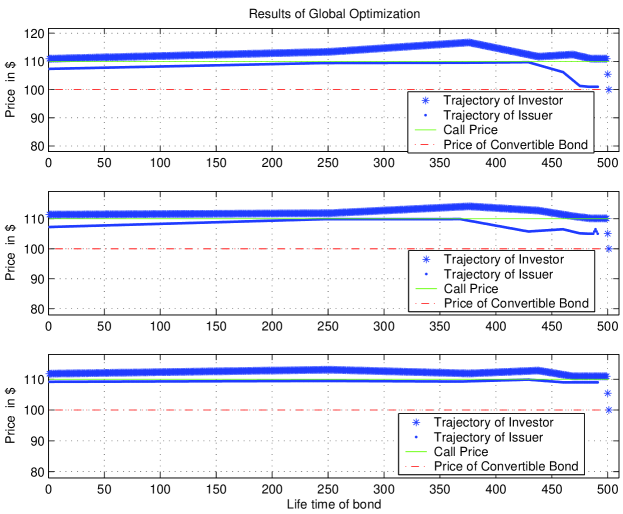
Figure 5. Strategies of Investor and Issuer. Different initial trajectories.

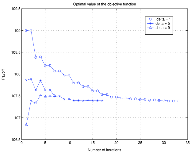
Figure 6. Objective function history. Different initial trajectories

Figure 6 shows that all three experiments terminate with the same objective function value, but give different points (strategies), see Figure 5.

The case with $\varepsilon=1$ requires the maximal number of iterations (almost twice as many as the case for $\varepsilon=5$ and three times as many as for $\varepsilon=10$).

The case with $\varepsilon=9$ seems to be not very informative, since almost nothing happens close to the maturity (see Figure 5, subplot 3).

So, the most interesting cases are $\varepsilon=1$ and $\varepsilon=5$, but we choose $\varepsilon=5$ in the basic set because in this case the number of iterations is twice lower in comparison with the case $\varepsilon=1$, and it produces an acceptable result.

3.4. Experiment 4: Different sizes of the problem

Instead of using the whole trajectories for issuers and investors, we used the approximated trajectories, see Section 2.4. The amount of points in (13) which gives a reasonable solution to the problem is the subject of investigation in this experiment.

We solved our problem for different sizes of the problem: $m=5,10$ and $15$. The rest of the parameters are (15)-(16) and (18).

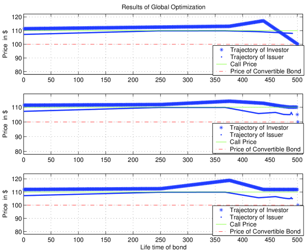
Figure 7. Strategies of Investor and Issuer. Different problem sizes

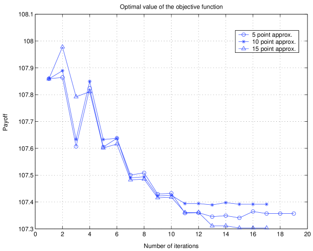
Figure 8. Objective function history. Different problem sizes

Figure 8 shows that the objective function history for all the cases is almost similar.

Nevertheless, $5$-point approximation of the strategies is not sufficient. Since the most interesting part of the strategy is the second, it is not enough to have only 3 points for approximation of the second part of the strategy. As seen from subplot 1, Figure 7, the strategies are not smooth enough in the vicinity of the maturity time.

$15$-point approximation gives very interesting results, but the size of the problem becomes too high as well. So, the best choice for the basic set is $10$-points approximation of the strategies, which is the tradeoff between two other approximations.

4. Conclusions and Suggestions for Further Investigation

In this study we considered a method for computing the strategies of the investor and the issuer dealing with convertible bonds. This method consists of two main stages: stock price generating and solution of the min-max optimization problem. For stock price generating we used a Monte-Carlo method based on the formula (4), and applied the Downhill Simplex method for the solution of the global nonlinear optimization problem. The results of our investigation allow to draw the following conclusions.

• The proposed method is sensitive to the number of generated trajectories of Stock Price. It means that for some small number of generated trajectories the method does not produce any reasonable solution. We suggest 500 trajectories as the minimal number required for achieving a reasonable solution (see Section 3.1);

• The Simplex Downhill method is sensitive to the size of the initial simplex. It is very important to choose the initial simplex of a proper size, otherwise there exists a risk to get non-acceptable solution, see Section 3.2. We recommend the size of simplex $k=3$.

• The Downhill Simplex is also sensitive to the choice of a good initial guess. The best choice in our experiments was $\varepsilon=5$ (see Section 3.3);

• The dimensions (size of the problem) is important in our experiments, too. Very large size of the problem requires too much computational time, but for a small size we get non-acceptable solution. We took 10 points (solved $10$-dimensional problem), see Section 3.4.

For further investigation the following is to be taken into account:

All the results presented in this study were obtained for predetermined constant values such as initial stock price, call price, face value of convertible bond, etc. So, it is very interesting to run experiments with other values of the economic parameters. Also, such parameters as volatility, interest rate, dividend yield may vary during the lifetime of the bond. For example, they may be recalculated every day, which will make stock price generation more complicated. Finally, the problem may be solved for nonzero coupon bond.

We used Brownian type stock price generation without jumps (see Section 2.1) which is one of the options. It is possible to consider some other stock price generation algorithms which have another nature (with jumps) and may give an interesting effect on the results.

From the viewpoint of the optimization it would be extremely useful to consider another global solver, since Downhill Simplex is so sensitive to the choice of the initial point and the size of initial simplex. On the other hand, some local optimization methods may be useful, since the problem is constrained and the feasibility area is quit narrow.

For more efficient strategies approximation it may be very helpful to consider other distribution of points (e.g. equidistant distribution) and other ways of approximation, e.g. cubic splines.

REFERENCES

-
AmmanM.KindA.WildeC.Simulation-based princing of convertible bondsJournal of Empirical Finance(2007)@article{ref1,
author = {Amman, M.},
author = {Kind, A.},
author = {Wilde, C.},
title = {Simulation-Based Princing of Convertible Bonds},
journal = {Journal of Empirical Finance},
year = {(2007)}}
- [2]
- [3] GarciaD.Convergence and biases of monte carlo estimates of american option prices using a parametric exercise ruleJournal of Economic Dynamics Control(2003)271855–1879@article{ref2, author = {Garcia, D.}, title = {Convergence and Biases of Monte Carlo estimates of American option prices using a parametric exercise rule}, journal = {Journal of Economic Dynamics $\&$ Control}, year = {(2003)}, volume = {27}, pages = {1855-1879}} IsakssonC.Pricing convertible bonds with monte carlo simulationsMälardalen University Master Thesis(2006)@thesis{ref25, author = {Isaksson, C.}, title = {Pricing Convertible Bonds with Monte Carlo simulations}, school = {M\"alardalen University Master Thesis}, year = {(2006)}}
- [6] NelderJ. A.MeadR.A simplex method for function minimizationThe Computer Journal(1964) volume = 7308–313@article{ref3, author = {Nelder, J. A.}, author = {Mead, R.}, title = {A simplex method for function minimization}, journal = {The Computer Journal}, year = {{(1964)} volume = {7}}, pages = {308-313}}
- [8]
- [9] PressW. H.TeukolskyS. A.VetterlingW. T.FlanneryB. P.Numerical recipes in c. the art of scientific computing. second edition Cambridge University Press(1997)@book{ref4, author = {Press, W. H. }, author = {Teukolsky, S. A.}, author = {Vetterling, W. T. }, author = {Flannery, B. P.}, title = {Numerical Recipes in C. The Art of Scientific Computing. Second Edition}, publisher = { Cambridge University Press}, date = {(1997)}}
- [11]