Geometry of Moving Planes

Abstract

The concept of number and its generalization has played a central role in the development of mathematics over many centuries and many civilizations. Noteworthy milestones in this long and arduous process were the developments of the real and complex numbers which have achieved universal acceptance. Serious attempts have been made at further extensions, such as Hamiltons quaternions, Grassmann’s exterior algebra and Clifford’s geometric algebra. By examining the geometry of moving planes, we show how new mathematics is within reach, if the will to learn these powerful methods can be found.

Introduction

Great advances in mathematics have been made by repeated extensions of the concept of number. The real number system $I\!\!R$ has a long and august history spanning a host of civilizations over many centuries. It is the rock upon which many other mathematical systems are constructed, and serves as a model of desirable properties that a number system should have. A property which the real number system does not have, the closure property for the zeros of any real polynomial, historically provided one the most compelling reasons for their extension. By extending the real numbers $I\!\!R$ to include an imaginary unit $i:=\sqrt{-1}\notin I\!\!R$, we arrive at the complex numbers $I\!\!\!C$. The complex numbers enjoy all the algebraic properties of the reals, but in addition are algebraically closed. Any complex number $z\in I\!\!\!C$ can be expressed in the standard basis $\{1,i\}_{I\!\!R}$ as $z=x+iy$ where $x,y\in I\!\!R$, leading to the idea of the $2$-dimensional complex number plane.

Over the last 150 years a rich complex analysis has been developed, which has been fully incorporated into the mathematical toolbox of every mathematician and practitioners of mathematics from the engineering and scientific communities. The famous Euler formula

$$\exp(i\theta)=\cos\theta+i\sin\theta$$ (1)

helps mades clear the geometric significance of the multiplication of complex numbers.

Whereas the complex numbers have enjoyed universal acceptance and admiration, other extensions have met with greater resistance and have found only limited acceptance. For example, the extension of the complex numbers to Hamilton’s quaternions, has been more divisive in its effects upon the mathematical community [3]. Other powerful extensions, such as Grassmann’s exterior algebras and William K. Clifford’s geometric algebras [2], have had a profound effect on the development of higher mathematics, but have yet to be brought into the mainstream of mathematics. A revealing history is told in [10, pp.320-327], and a website devoted to telling this fascinating story, with many references to the literature, can be found at (http://modelingnts.la.asu.edu/).

The principal roadblock to further extensions of the real number system has been the failure to consider the extension of the real numbers to include new square roots of $+1$, perhaps because such considerations were for the most part before the advent of Einstein’s theory of special relativity and the study of non-Euclidean geometries. Extending the real number system $I\!\!R$ to include a new square root $u=\sqrt{1}\notin I\!\!R$ leads to the concept of the hyperbolic number plane $I\!\!H$, which in many ways is analogous to the complex number plane $I\!\!\!C$. Understanding the hyperbolic numbers is key to understanding even more general geometric extensions of the real numbers.

A hyperbolic number $w\in I\!\!H$, in the standard basis $\{1,u\}_{I\!\!R}$, has the form $w=x+uy$ for $x,y\in I\!\!R$. The hyperbolic numbers $I\!\!H$ enjoy all the properties of the real numbers $I\!\!R$, except that $I\!\!H$ has zero divisors. The real hyperbolic numbers $I\!\!H$ have the structure of a commutative ring, but are not algebraically closed. It is interesting to note that the hyperbolic numbers, just like the complex numbers, can be used to derive the not-so-well known formula for the zeros of a real cubic polynomial [13].

The Euler forms of a hyperbolic number $w=x+uy\in I\!\!H$ are $w=\pm\rho\exp{u\phi}$ or $w=\pm\rho u\exp{u\phi}$ for $\rho=\sqrt{|x^{2}-y^{2}|}$ and $\phi=Tanh^{-1}(y/x)$ or $\phi=Tanh^{-1}(x/y)$, respectively, corresponding to the $4$ branches of the unit hyperbola $x^{2}-y^{2}=\pm 1$. Expanding $e^{u\phi}$ in terms of the hyperbolic trig functions gives

$$e^{u\phi}=\cosh\phi+u\sinh\phi,$$ (2)

which of course is analogous to (1). The Euler forms facilitate the geometric interpretation of the multiplication of hyperbolic numbers. For example, if $w_{1}=\rho_{1}e^{u\phi_{1}}$ and $w_{2}=\rho_{2}e^{u\phi_{2}}$, then

$$w_{1}w_{2}=\rho_{1}\rho_{2}e^{u(\phi_{1}+\phi_{2})}.$$

The hyperbolic distance between $w_{1},w_{2}\in I\!\!H$ is defined by

$$|w_{1}-w_{2}|=\sqrt{|(x_{1}-x_{2})^{2}-(y_{1}-y_{2})^{2}|},$$

and the equation of the hyperbola with hyperbolic radius $\rho$ is $|ww^{-}|=|x^{2}-y^{2}|=\rho^{2}$, where $w^{-}:=x-yu$.

The defect that the hyperbolic numbers are not algebraically closed can be remedied by introducing the $4$-dimensional complex hyperbolic numbers. But instead, following William Kingdon Clifford [2], we will consider the extension of the real numbers obtained by introducing two anticommuting square roots of $+1$.

Geometric numbers of the $2$-plane

To obtain the associative geometric algebra $I\!\!\!G_{2}$ of the Euclidean plane $I\!\!R^{2}$, we extend the real numbers $I\!\!R$ to include two new anticommuting square roots ${\bf e}_{1}$ and ${\bf e}_{2}$ of $+1$, so that

$$I\!\!\!G_{2}=span\{1,{\bf e}_{1},{\bf e}_{2},{\bf e}_{12}\}_{I\!\!R},$$

where ${\bf e}_{1}^{2}={\bf e}_{2}^{2}=1$ and ${\bf e}_{12}:={\bf e}_{1}{\bf e}_{2}=-{\bf e}_{2}{\bf e}_{1}$. We say that

$${\cal B}:=\{1,{\bf e}_{1},{\bf e}_{2},{\bf e}_{1}{\bf e}_{2}\}$$ (3)

is a standard orthonormal basis of $I\!\!\!G_{2}$, where ${\bf e}_{1}$ and ${\bf e}_{2}$ are given the interpretation of orthonormal vectors along the $x$ and $y$ axis of $I\!\!R^{2}$, respectively. The quantity $i:={\bf e}_{12}$ has the geometric interpretation of a unit bivector, and defines the direction and orientation of the vector plane $I\!\!R^{2}$. See Figure 1. The geometric algebra $I\!\!\!G_{2}$ obeys all the algebraic rules of the real numbers $I\!\!R$, except that $I\!\!\!G_{2}$ has zero divisors and is not universally commutative.

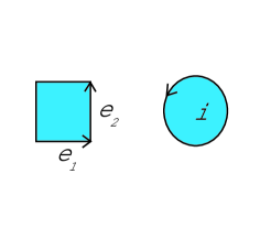
Figure 1: The unit bivector $i$ of $I\!\!R^{2}$.

Calculating

$$i^{2}=({\bf e}_{1}{\bf e}_{2})({\bf e}_{1}{\bf e}_{2})=-{\bf e}_{1}({\bf e}_{1}{\bf e}_{2}){\bf e}_{2}=-{\bf e}_{1}^{2}{\bf e}_{2}^{2}=-1,$$

we see that $i$ has the same algebraic property as the imaginary unit of the complex numbers. The most general geometric number $g\in I\!\!\!G_{2}$ has the form

$$g=(x+iy)+(v_{1}{\bf e}_{1}+v_{2}{\bf e}_{2})=z+{\bf v},$$ (4)

where the spinor $z=x+iy$ for $x,y\in I\!\!R$ behaves like a complex number, and ${\bf v}=v_{1}{\bf e}_{1}+v_{2}{\bf e}_{2}\in I\!\!R^{2}$ is a vector in the two dimensional Euclidean space $I\!\!R^{2}$. We say that $z\in{\cal S}_{i}$ where ${\cal S}_{i}$ is the spinor plane of the bivector $i={\bf e}_{1}{\bf e}_{2}$. Noting that

$${\bf e}_{1}i={\bf e}_{1}{\bf e}_{1}{\bf e}_{2}={\bf e}_{2},\ {\rm and}\ {\bf e}_{2}i={\bf e}_{2}{\bf e}_{1}{\bf e}_{2}=-{\bf e}_{1}$$ (5)

it follows that multiplying any vector ${\bf v}\in I\!\!R^{2}$ on the right by $i$ rotates the vector $\pi/2$ radians counterclockwise in the plane of bivector $i$. Consequently, the spinors $e^{i\theta}$ generate rotations in the oriented vector plane of $I\!\!R^{2}$.

Let ${\bf a},{\bf b}\in I\!\!R^{2}$ be two unit vectors so that ${\bf a}^{2}={\bf b}^{2}=1$. Then

$${\bf a}{\bf b}={\bf a}\cdot{\bf b}+{\bf a}\wedge{\bf b}=\cos\theta+i\sin\theta=e^{i\theta},$$ (6)

where ${\bf a}\cdot{\bf b}:=\frac{1}{2}({\bf a}{\bf b}+{\bf b}{\bf a})=\cos\theta$ is the symmetric inner product and ${\bf a}\wedge{\bf b}:=\frac{1}{2}({\bf a}{\bf b}-{\bf b}{\bf a})=i\sin\theta$ is the anti-symmetric outer product of the vectors ${\bf a}$ and ${\bf b}$. The equation (6) shows the deep relationship that exists between the vectors of $I\!\!R^{2}$ and the spinors ${\cal S}_{i}$ of $I\!\!R^{2}$. We write $I\!\!R^{2}=I\!\!R_{i}^{2}$ to emphasize that $I\!\!R^{2}$ consists of all vectors in the plane of the bivector $i={\bf e}_{1}{\bf e}_{2}$.

Let ${\bf x}\in I\!\!R^{2}$. Since

$${\bf b}=({\bf b}{\bf a}){\bf a}=({\bf b}{\bf a})^{\frac{1}{2}}{\bf a}({\bf a}{\bf b})^{\frac{1}{2}}=e^{-\frac{i\theta}{2}}{\bf a}e^{\frac{i\theta}{2}},$$

it follows that

$${\bf x}^{\prime}=R({\bf x})=({\bf b}{\bf a})^{\frac{1}{2}}{\bf x}({\bf a}{\bf b})^{\frac{1}{2}}=e^{-\frac{i\theta}{2}}{\bf x}e^{\frac{i\theta}{2}}$$ (7)

defines a rotation of the vector ${\bf x}$ in the plane of the bivector $i={\bf e}_{1}{\bf e}_{2}$ into the vector ${\bf x}^{\prime}$, and in particular $R({\bf a})={\bf b}$. When applied to the bivector $i={\bf e}_{1}{\bf e}_{2}$ we find that $R(i)=i$, so that a rotation of the bivector $i$ in the plane of $i$ leaves the bivector unchanged, as expected. Note that the half-angle version on the right hand side of (7) is useful because it extends immediately to rotations in $I\!\!R^{n}$. See [9] and [10] for an extensive treatment of geometric algebras in higher dimensional pseudo-Euclidean spaces.

The geometric algebra $I\!\!\!G_{2}$ algebraically unites the spinor plane ${\cal S}_{i}$ and the vector plane $I\!\!R_{i}^{2}$ and opens up many new possibilities. Consider the transformation $L({\bf x})$ defined by

$${\bf x}^{\prime}=L({\bf x})=e^{-\frac{\phi{\bf a}}{2}}{\bf x}e^{\frac{\phi{\bf a}}{2}}$$ (8)

for a unit vector ${\bf a}\in I\!\!R^{2}$. The transformation (8) has the same half-angle form as the rotation (7). We say that (8) defines an active Lorentz boost of the vector ${\bf x}$ into the relative vector ${\bf x}^{\prime}$ moving with velocity

$$\frac{{\bf v}}{c}=\tanh{(\phi{\bf a})}={\bf a}\tanh\phi$$

where $c$ is the velocity of light. For simplicity we shall always take $c=1$. An active rotation and an active boost are pictured in Figure 2.

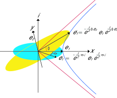
Figure 2: An active rotation and an active boost.

Both $R({\bf x})$ and $L({\bf x})$ are algebra inner automorphisms on $I\!\!\!G_{2}$, satisfying $R(g_{1}g_{2})=R(g_{1})R(g_{2})$ and $L(g_{1}g_{2})=L(g_{1})L(g_{2})$ for all $g_{1},g_{2}\in I\!\!R^{2}$. In addition, we say that $R({\bf x})$ is an outermorphism because it preserves the grading of the algebra $I\!\!\!G_{2}$, i.e., for ${\bf x}\in I\!\!R^{2}$, $R({\bf x})\in I\!\!R^{2}$. Whereas a boost is an automorphism, it is not an outermorphism as we shall shortly see.

Note that under both a Euclidean rotation (7) and under an active boost (8),

$$|{\bf x}^{\prime}|^{2}:=({\bf x}^{\prime})^{2}={\bf x}^{2}:=|{\bf x}|^{2},$$

so that the Euclidean lengths $|{\bf x}|=|{\bf x}^{\prime}|$ of both the rotated vector and the boosted relative vector are preserved . Whereas the meaning of this statement is well-known for rotations, the corresponding statement for a boost needs further explanation.

The active boost (8) leaves invariant the direction of the boost, that is

$$L({\bf a})=e^{-\frac{\phi{\bf a}}{2}}{\bf a}e^{\frac{\phi{\bf a}}{2}}={\bf a}.$$ (9)

On the other hand, for the vector ${\bf a}i$ orthogonal to ${\bf a}$, we have

$$L({\bf a}i)=e^{-\frac{\phi{\bf a}}{2}}{\bf a}ie^{\frac{\phi{\bf a}}{2}}={\bf a}ie^{\phi{\bf a}}={\bf a}i\cosh\phi-i\sinh\phi,$$ (10)

showing that the boosted relative vector $L({\bf a}i)$ has picked up the bivector component $-i\sinh\phi$.

We say that two relative vectors are orthogonal if they are anticommutative. From the calculation

$$L({\bf a})L({\bf a}i)={\bf a}{\bf a}ie^{\phi{\bf a}}=-{\bf a}ie^{\phi{\bf a}}{\bf a}=-L({\bf a}i)L({\bf a}),$$ (11)

we see that the active boost of a pair orthornormal vectors gives a pair of orthornormal relative vectors. When the active Lorentz boost is applied to the bivector $i={\bf e}_{1}{\bf e}_{2}$ we find that $j=L(i)=ie^{{\bf a}\phi}$, so that a boost of the bivector $i$ in the direction of the vector ${\bf a}$ gives the relative bivector $j=ie^{{\bf a}\phi}$. Note that

$$j^{2}=ie^{{\bf a}\phi}ie^{{\bf a}\phi}=i^{2}e^{-{\bf a}\phi}e^{{\bf a}\phi}=-1$$

as expected.

Using equations (9), (10) and (11), we say that

$${\cal B}_{j}:=\{1,{\bf e}_{1}^{\prime},{\bf e}_{2}^{\prime},{\bf e}_{1}^{\prime}{\bf e}_{2}^{\prime}\},$$

where ${\bf e}_{1}^{\prime}={\bf a}$, ${\bf e}_{2}^{\prime}={\bf a}ie^{\phi{\bf a}}$, and $j={\bf a}{\bf a}ie^{\phi{\bf a}}=ie^{\phi{\bf a}}$, makes up a relative orthonormal basis of $I\!\!\!G_{2}$. Note that the defining rules for the standard basis (3) of $I\!\!\!G_{2}$ remain the same for the relative basis ${\cal B}_{j}$:

$$({\bf e}_{1}^{\prime})^{2}=({\bf e}_{2}^{\prime})^{2}=1,\ {\rm and}\ {\bf e}_{1}^{\prime}{\bf e}_{2}^{\prime}=-{\bf e}_{2}^{\prime}{\bf e}_{1}^{\prime}.$$

Essentially, the relative basis ${\cal B}_{j}$ of $I\!\!\!G_{2}$ regrades the algebra into relative vectors and relative bivectors moving at the velocity of ${\bf v}={\bf a}\tanh\phi$ with respect to the standard basis ${\cal B}_{i}$. We say that $j$ defines the direction and orientation of the relative plane

$${I\!\!R_{j}^{2}}:=\{{\bf v}^{\prime}|\ \ {\bf v}^{\prime}=x^{\prime}{\bf e}_{1}^{\prime}+y^{\prime}{\bf e}_{2}^{\prime},{\rm for}\ \ x^{\prime},y^{\prime}\in I\!\!R\}.$$ (12)

Active rotations (7) and active boosts (8) define two different kinds of automorphisms on the geometric algebra $I\!\!\!G_{2}$. Whereas active rotations are well understood in Euclidean geometry, an active boost brings in concepts from non-Euclidean geometry. Since an active boost essentially regrades the geometric algebra $G_{2}$ into relative vectors and relative bivectors, it is natural to refer to the relative geometric algebra $I\!\!\!G_{2}$ of the relative plane (12) when using this basis.

Relative geometric algebras

We have seen that both the unit bivector $i$ and the relative unit bivector $j=ie^{{\bf a}\phi}$ have square $-1$. Let us see what can be said about the most general element $h\in I\!\!\!G_{2}$ which has the property that $h^{2}=-1$. In the standard basis (3), $h$ will have the form

$$h=h_{1}{\bf e}_{1}+h_{2}{\bf e}_{2}+h_{3}i$$

for $h_{1},h_{2},h_{3}\in I\!\!R$ as is easily verified. Clearly the condition that $h^{2}=h_{1}^{2}+h_{2}^{2}-h_{3}^{2}=-1$ will be satisfied if and only if $1+h_{1}^{2}+h_{2}^{2}=h_{3}^{2}$ or $h_{3}=\pm\sqrt{1+h_{1}^{2}+h_{2}^{2}}$. We have two cases:

• If $h_{3}\geq 0$, define $\cosh\phi=\sqrt{1+h_{1}^{2}+h_{2}^{2}}$, $\sinh\phi=\sqrt{h_{1}^{2}+h_{2}^{2}}$ and the unit vector ${\bf a}$ such that $i{\bf a}\sinh\phi=h_{1}{\bf e}_{1}+h_{2}{\bf e}_{2}$, or ${\bf a}=\frac{h_{1}{\bf e}_{2}-h_{2}{\bf e}_{1}}{\sqrt{1+h_{1}^{2}+h_{2}^{2}}}$. Defined in this way, $h=ie^{{\bf a}\phi}$ is a relative bivector to $i$.

• If $h_{3}<0$, define $\cosh\phi=\sqrt{1+h_{1}^{2}+h_{2}^{2}}$, $\sinh\phi=-\sqrt{h_{1}^{2}+h_{2}^{2}}$ and the unit vector ${\bf a}$ such that $i{\bf a}\sinh\phi=-(h_{1}{\bf e}_{1}+h_{2}{\bf e}_{2})$, or ${\bf a}=\frac{h_{1}{\bf e}_{2}-h_{2}{\bf e}_{1}}{\sqrt{1+h_{1}^{2}+h_{2}^{2}}}$. In this case, $h=-ie^{{\bf a}\phi}$ is a relative bivector to $-i$.

From the above remarks we see that any geometric number $h\in G_{2}$ with the property that $h^{2}=-1$ is a relative bivector to $\pm i$. The set of relative bivectors to $+i$,

$${\cal H}^{+}:=\{ie^{\phi{\bf a}}|\ \ {\bf a}={\bf e}_{1}\cos\theta+{\bf e}_{2}\sin\theta,\ 0\leq\theta<2\pi,\ \phi\in I\!\!R\}$$ (13)

are said to be positively oriented . Moving relative bivectors $i$, $j$ and $k$ are pictured in Figure 3. Similarly, the set ${\cal H}^{-}$ of negatively oriented relative bivectors to $-i$ can be defined.

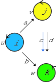
Figure 3: The moving relative bivectors $i$, $j$ and $k$.

For each positively oriented relative bivector $h=ie^{{\bf a}\phi}\in{\cal H}^{+}$, we define a positively oriented relative plane $I\!\!R_{h}^{2}$ by

$$I\!\!R_{h}^{2}=\{{\bf x}|\ \ {\bf x}=x{\bf a}+y{\bf a}i,\ x,y\in I\!\!R\},$$

and the corresponding relative basis ${\cal B}_{h}$ of the geometric algebra $I\!\!\!G_{2}$:

$${\cal B}_{h}=\{1,{\bf a},{\bf a}ie^{{\bf a}\phi},ie^{{\bf a}\phi}\}.$$

In Figure 3, we have also introduced the symbols $u$, $v$ and $w$ to label the systems or oriented frames defined by the relative bivectors $i$, $j$ and $k$, respectively. These symbols will later take on an algebraic interpretation as well.

For each relative plane $I\!\!R_{h}^{2}$ there exist a relative inner product and a relative outer product, just as in (6). Rather than use the relative inner and outer products on each different relative plane, we prefer to decompose the geometric product of two elements $g_{1},g_{2}\in G_{2}$ into symmetric and anti-symmetric parts. Thus,

$$g_{1}g_{2}=\frac{1}{2}(g_{1}g_{2}+g_{2}g_{1})+\frac{1}{2}(g_{1}g_{2}+g_{2}g_{1})=g_{1}\circ g_{2}+g_{1}\otimes g_{2}$$ (14)

where $g_{1}\circ g_{2}=\frac{1}{2}(g_{1}g_{2}+g_{2}g_{1})$ is called the symmetric product and $g_{1}\otimes g_{2}=\frac{1}{2}(g_{1}g_{2}-g_{2}g_{1})$ is called the anti-symmetric product.

We give here formulas for evaluating the symmetric and anti-symmetric products of geometric numbers with vanishing scalar parts. Letting $A=a_{1}{\bf e}_{1}+a_{2}{\bf e}_{2}+a_{3}i$, $B=b_{1}{\bf e}_{1}+b_{2}{\bf e}_{2}+b_{3}i$, and $C=c_{1}{\bf e}_{1}+c_{2}{\bf e}_{2}+c_{3}i$, we have

$$A\circ B=a_{1}b_{1}+a_{2}b_{2}-a_{3}b_{3}$$

$$A\otimes B=-\det{\pmatrix{{\bf e}_{1}&{\bf e}_{2}&-i\cr a_{1}&a_{2}&a_{3}\cr b_{1}&b_{2}&b_{3}}}$$

$$A\circ(B\otimes C)=-\det{\pmatrix{a_{1}&a_{2}&a_{3}\cr b_{1}&b_{2}&b_{3}\cr c_{1}&c_{2}&c_{3}}},$$

which bear striking resemblance to the dot and cross products of vector analysis. In general, a nonzero geometric number $A\in I\!\!\!G_{2}$ with vanishing scalar part is said to be a relative vector if $A^{2}>0$, a nilpotent if $A^{2}=0$, and a relative bivector if $A^{2}<0$.

Geometry of moving planes

Consider the set ${\cal H}^{+}$ of positively oriented relative bivectors to $i$. For $j\in{\cal H}^{+}$, this means that $j=ie^{\phi{\bf a}}$ as given in (13). We say that the system $v$, and its relative plane $I\!\!R_{j}^{2}$ defined by the bivector $j$, is moving with velocity ${\bf u}_{v}:={\bf a}\tanh\phi$ with respect to the system $u$ and its relative plane $I\!\!R_{i}^{2}$ defined by the bivector $i$.

Note that $j=ie^{\phi{\bf a}}$ implies that $i=je^{-\phi{\bf a}}$, so that if $j$ is moving with velocity ${\bf u}_{v}={\bf a}\tanh\phi$ with respect to $i$, then $i$ is moving with velocity ${\bf v}_{u}=-{\bf a}\tanh\phi$ with respect to $j$. Suppose now for the system $w$ that $k=ie^{\rho{\bf b}}\in{\cal H}^{+}$, where the unit vector ${\bf b}\in I\!\!R_{i}^{2}$ and the hyperbolic angle $\rho\in I\!\!R$. Then

$$k=i(e^{\phi{\bf a}}e^{-\phi{\bf a}})e^{\rho{\bf b}}=j(e^{-\phi{\bf a}}e^{\rho{\bf b}})=je^{\omega{\bf c}},$$

where $e^{\omega{\bf c}}=e^{-\phi{\bf a}}e^{\rho{\bf b}}$ for some hyperbolic angle $\omega$ and relative unit vector ${\bf c}\in I\!\!R_{j}^{2}\cap I\!\!R_{k}^{2}$.

Expanding $e^{\omega{\bf c}}=e^{-\phi{\bf a}}e^{\rho{\bf b}}$, we get

$$\cosh\omega(1+{\bf v}_{w})=e^{-\phi{\bf a}}e^{{\bf b}}=\cosh\phi\cosh\rho(1-{\bf u}_{v})(1+{\bf u}_{w})$$

$$=\cosh\phi\cosh\rho[(1-{\bf u}_{v}\cdot{\bf u}_{w})+({\bf u}_{w}-{\bf u}_{v}-{\bf u}_{v}\wedge{\bf u}_{w})].$$

It follows that

$$\cosh\omega=(\cosh\phi\cosh\rho)(1-{\bf u}_{v}\cdot{\bf u}_{w}),$$ (15)

and

$${\bf v}_{w}=\frac{\cosh\phi\cosh\rho}{\cosh\omega}({\bf u}_{w}-{\bf u}_{v}-{\bf u}_{v}\wedge{\bf u}_{w})=\frac{{\bf u}_{w}-{\bf u}_{v}-{\bf u}_{v}\wedge{\bf u}_{w}}{1-{\bf u}_{v}\cdot{\bf u}_{w}}.$$ (16)

We have found a relative unit vector ${\bf c}\in I\!\!R_{j}^{2}\cap I\!\!R_{k}^{2}$, ${\bf c}:=\frac{{\bf v}_{w}}{\tanh\omega}$ and a hyperbolic angle $\omega\geq 0$ with the property that

$$k=je^{\omega{\bf c}}=e^{-\frac{1}{2}\omega{\bf c}}je^{\frac{1}{2}\omega{\bf c}}.$$

The relative bivector $k$ has velocity ${\bf v}_{w}={\bf c}\tanh\omega$ with respect to the $j$. However, the relative unit vector ${\bf c}\notin I\!\!R_{i}^{2}$. This means that the relative vector ${\bf c}$ defining the direction of the velocity of the relative bivector $k$ with respect to $j$ is not commensurable with the vectors in $I\!\!R_{i}^{2}$.

The question arises whether or not there exist a unit vector ${\bf d}\in I\!\!R_{i}^{2}$ with the property that

$$k=e^{-\frac{1}{2}\Omega{\bf d}}je^{\frac{1}{2}\Omega{\bf d}}.$$ (17)

Substituting $j=ie^{\phi{\bf a}}$ and $k=ie^{\rho{\bf b}}$ into this last equation gives

$$ie^{\rho{\bf b}}=e^{-\frac{1}{2}\Omega{\bf d}}ie^{\phi{\bf a}}e^{\frac{1}{2}\Omega{\bf d}},$$

which is equivalent to the equation

$$e^{\rho{\bf b}}=e^{\frac{1}{2}\Omega{\bf d}}e^{\phi{\bf a}}e^{\frac{1}{2}\Omega{\bf d}}.$$ (18)

The transformation $L_{p}:I\!\!\!G_{2}->I\!\!\!G_{2}$ defined by

$$L_{p}({\bf x})=e^{\frac{1}{2}\Omega{\bf d}}{\bf x}e^{\frac{1}{2}\Omega{\bf d}}$$ (19)

is called the passive Lorentz boost relating $I\!\!R_{j}^{2}$ to $I\!\!R_{k}^{2}$ with respect to $I\!\!R_{i}^{2}$.

The equation (18) can either be solved for $e^{\rho{\bf b}}$ given $e^{\Omega{\bf d}}$ and $e^{\phi{\bf a}}$, or for $e^{\Omega{\bf d}}$ given $e^{\phi{\bf a}}$ and $e^{\rho{\bf b}}$. Defining the velocities ${\bf u}_{v}={\bf a}\tanh\phi,{\bf u}_{w}={\bf b}\tanh\rho$, and ${\bf u}_{vw}={\bf d}\tanh\Omega$, we first solve for $e^{\rho{\bf b}}$ given $e^{\Omega{\bf d}}$ and $e^{\phi{\bf a}}$. In terms of these velocities, equation (18) takes the form

$$\cosh\rho\ (1+{\bf u}_{w})=\cosh\phi\ e^{\frac{1}{2}\Omega{\bf d}}(1+{\bf u}_{v})e^{\frac{1}{2}\Omega{\bf d}}=\cosh\phi\ (e^{\Omega{\bf d}}+e^{\frac{1}{2}\Omega{\bf d}}{\bf u}_{v}e^{\frac{1}{2}\Omega{\bf d}})$$

$$=\cosh\phi\cosh\Omega\ [(1+{\bf u}_{vw})(1+{\bf u}_{v}^{\parallel})]+\cosh\phi\ {\bf u}_{v}^{\perp}$$

where ${\bf u}_{v}^{\parallel}=({\bf u}_{v}\cdot{\bf d}){\bf d}$ and ${\bf u}_{v}^{\perp}=({\bf u}_{v}\wedge{\bf d}){\bf d}$ . Equating scalar and vector parts gives

$$\cosh\rho=\cosh\phi\cosh\Omega\ (1+{\bf u}_{v}\cdot{\bf u}_{vw}),$$ (20)

and

$${\bf u}_{w}=\frac{{\bf u}_{v}+{\bf u}_{vw}+(\frac{1}{\cosh\Omega}-1)({\bf u}_{v}\wedge{\bf d}){\bf d}}{1+{\bf u}_{v}\cdot{\bf u}_{vw}}.$$ (21)

The equation (21) is the (passive) composition formula for the addition of velocities of special relativity in the system $u$, [7, p.588] and [10, p.133].

To solve (18) for $e^{\Omega{\bf d}}$ given $e^{\phi{\bf a}}$ and $e^{\rho{\bf b}}$, we first solve for the unit vector ${\bf d}\in I\!\!R^{2}$ by taking the anti-symmetric product of both sides of (18) with ${\bf d}$ to get the relationship

$${\bf d}\otimes{\bf b}\ \sinh\rho=e^{\frac{1}{2}\Omega{\bf d}}{\bf d}\otimes{\bf a}\ \sinh\phi\ e^{\frac{1}{2}\Omega{\bf d}}={\bf a}\sinh\phi,$$

or equivalently,

$${\bf d}\wedge({\bf b}\sinh\rho-{\bf a}\sinh\phi)=0.$$

In terms of the velocity vectors ${\bf u}_{v}$ and ${\bf u}_{w}$, we can define the unit vector ${\bf d}$ by

$${\bf d}=\frac{{\bf u}_{w}\cosh\rho-{\bf u}_{v}\cosh\phi}{\sqrt{{\bf u}_{v}^{2}\cosh^{2}\phi-2{\bf u}_{v}\cdot{\bf u}_{w}\cosh\phi\cosh\rho+{\bf u}_{w}^{2}\cosh^{2}\rho}}$$ (22)

Taking the symmetric product of both sides of (18) with ${\bf d}$ gives

$$[{\bf d}\circ e^{\phi{\bf a}}]e^{\Omega{\bf d}}={\bf d}\circ e^{\rho{\bf b}},$$

or

$$({\bf d}\cosh\phi+{\bf a}\cdot{\bf d}\sinh\phi)e^{\Omega{\bf d}}={\bf d}\cosh\rho+{\bf b}\cdot{\bf d}\sinh\rho.$$

Solving this last equation for $e^{\Omega{\bf d}}$ gives

$$e^{\Omega{\bf d}}=\frac{({\bf d}\cosh\rho+{\bf b}\cdot{\bf d}\sinh\rho)({\bf d}\cosh\phi-{\bf a}\cdot{\bf d}\sinh\phi)}{\cosh^{2}\phi-({\bf a}\cdot{\bf d})^{2}\sinh^{2}\phi},$$ (23)

or in terms of the velocity vectors,

$$\cosh\Omega(1+{\bf u}_{vw})=\frac{\cosh\rho}{\cosh\phi}\Big{(}\frac{(1+{\bf u}_{w}\cdot{\bf d}\ {\bf d})(1-{\bf u}_{v}\cdot{\bf d}\ {\bf d})}{1-({\bf u}_{v}\cdot{\bf d})^{2}}\Big{)}$$

$$=\frac{\cosh\rho}{\cosh\phi}\Big{(}\frac{1-({\bf u}_{v}\cdot{\bf d})({\bf u}_{w}\cdot{\bf d})+({\bf u}_{w}-{\bf u}_{v})\cdot{\bf d}\ {\bf d}}{1-({\bf u}_{v}\cdot{\bf d})^{2}}\Big{)}.$$

Taking scalar and vector parts of this last equation gives

$$\cosh\Omega=\frac{\cosh\rho}{\cosh\phi}\Big{(}\frac{1-({\bf u}_{v}\cdot{\bf d})({\bf u}_{w}\cdot{\bf d})}{1-({\bf u}_{v}\cdot{\bf d})^{2}}\Big{)}$$ (24)

and

$${\bf u}_{vw}=\frac{({\bf u}_{w}-{\bf u}_{v})\cdot{\bf d}\ {\bf d}}{1-({\bf u}_{v}\cdot{\bf d})({\bf u}_{w}\cdot{\bf d})}.$$ (25)

We say that ${\bf u}_{vw}$ is the relative velocity of the passive boost (19) of $j$ into $k$ relative to $i$. The passive boost is at the foundation of the Algebra of Physical Space formulation of special relativity [1], and a coordinate form of this passive approach was used by Einstein in his famous 1905 paper [4]. Whereas Hestenes in [8] employs the active Lorentz boost, in [7] he uses the passive form of the Lorentz boost.

The distinction between active and passive boosts continues to be the source of much confusion in the literature [11]. Whereas an active boost (8) mixes vectors and bivectors of $I\!\!\!G_{2}$, the passive boost defined by (19) mixes the vectors and scalars of $I\!\!\!G_{2}$ in the geometric algebra $I\!\!\!G_{2}$ of $i$. In the next section, we shall find an interesting geometric interpretation of this result in a closely related higher dimensional space.

Splitting the plane

Geometric insight into the previous calculations can be obtained by splitting or factoring the geometric algebra $I\!\!\!G_{2}$ into a larger geometric algebra $I\!\!\!G_{1,2}$. The most mundane way of accomplishing this is to factor the standard orthonormal basis vectors of (3) into an orthonormal bivectors of a larger geometric algebra $I\!\!\!G_{1,2}$. We write

$${\bf e}_{1}=\gamma_{0}\gamma_{1},\ \ {\rm and}\ \ {\bf e}_{2}=\gamma_{0}\gamma_{2},$$

and assume the rules $\gamma_{0}^{2}=1=-\gamma_{1}^{2}=-\gamma_{2}^{2}$, and $\gamma_{\mu}\gamma_{\eta}=-\gamma_{\eta}\gamma_{\mu}$ for all $\mu,\eta=0,1,2$ and $\mu\neq\eta$. The standard orthonormal basis of $I\!\!\!G_{1,2}$ consists of the eight elements

$$\{1,\gamma_{0},\gamma_{1},\gamma_{2},\gamma_{01},\gamma_{02},\gamma_{21},\gamma_{012}\}.$$

With this splitting, the standard basis elements (3) of $I\!\!\!G_{2}$ are identified with elements of the even subalgebra

$$I\!\!\!G_{2,1}^{+}:=span\{1,{\bf e}_{1}=\gamma_{01},{\bf e}_{2}=\gamma_{02},{\bf e}_{12}=\gamma_{21}\}$$ (26)

of $I\!\!\!G_{1,2}$. We denote the oriented unit pseudoscalar element by $s=\gamma_{012}$. Note that $s\in Z(I\!\!\!G_{1,2})$, the center of the algebra $I\!\!\!G_{1,2}$.

Consider now the mapping

$$\psi:{\cal H}^{+}\longrightarrow\{r\in I\!\!\!G_{1,2}^{1}|\ \ r^{2}=1\}$$ (27)

defined by $r=\psi(h)=sh$ for all $h\in{\cal H}^{+}$. The mapping $\psi$ sets up a $1-1$ correspondence between the positively oriented unit bivectors $h\in{\cal H}^{+}$ and unit timelike vectors $r\in I\!\!\!G_{1,2}^{1}$ which are dual under multiplication by the pseudosclar $s$. Suppose now that $\psi(i)=u$, $\psi(j)=v$ and $\psi(k)=k$. Then it immediately follows by duality that if $j=ie^{\phi{\bf a}}$, $k=ie^{\rho{\bf b}}$ and $k=je^{\omega{\bf c}}$, then $v=ue^{\phi{\bf a}}$, $w=ue^{\phi{\bf a}}$ and $w=ve^{\omega{\bf c}}$, respectively. It is because of this $1-1$ correspondence that we have included the labels $u$, $v$ and $w$ as another way of identifying the oriented planes of the bivectors $i$, $j$ and $k$ in Figure 3.

Just as vectors in ${\bf x},{\bf y}\in I\!\!\!G_{2}^{1}$ are identified with points ${\bf x},{\bf y}\in I\!\!R^{2}$, Minkowski vectors $x,y\in I\!\!\!G_{1,2}^{1}$ are identified with points $x,y\in I\!\!R^{1,2}$ the $3$-dimensional pseudoeuclidean space of the Minkowski spacetime plane. A Minkowski vector $x\in I\!\!R^{1,2}$ is said to be timelike if $x^{2}>0$, spacelike if $x^{2}<0$, and lightlike if $x\neq 0$ but $x^{2}=0$. For two Minkowski vectors $x,y\in G_{1,2}^{1}$, we decompose the geometric product $xy$ into symmetric and anti-symmetric parts

$$xy=\frac{1}{2}(xy+yx)+\frac{1}{2}(xy-yx)=x\cdot y+x\wedge y,$$

where $x\cdot y:=\frac{1}{2}(xy+yx)$ is called the Minkowski inner product and $x\wedge y:=\frac{1}{2}(xy-yx)$ is called the Minkowski outer product to distinquish these products from the corresponding inner and outer products defined in $I\!\!\!G_{2}$.

In [6] and [8], David Hestenes gives an active reformulation of Einstein’s special relativity in the spacetime algebra $I\!\!\!G_{1,3}$. In [14, 15], I show that an equivalent active reformulation is possible in the geometric algebra $I\!\!\!G_{3}$ of the Euclidean space $I\!\!R^{3}$. In [1] and [5] the relationship between active and passive formulations is considered.

For the two unit timelike vectors $u,v\in I\!\!\!G_{1,2}$, we have

$$uv=u\cdot v+u\wedge v=e^{\phi{\bf a}}=\cosh\phi+{\bf a}\sinh\phi.$$ (28)

It follows that $u\cdot v=\cosh\phi$ and $u\wedge v={\bf a}\sinh\phi$, which are the hyperbolic counterparts to the geometric product of unit vectors ${\bf a},{\bf b}\in I\!\!R^{2}$ given in (6). The Minkowski bivector

$${\bf u}_{v}=\frac{u\wedge v}{u\cdot v}={\bf a}\tanh\phi=-{\bf v}_{u}$$

is the relative velocity of the timelike vector unit vector $v$ in the frame of $u$.

Suppose now that for $i,j,k\in{\cal H}^{+}$, $\psi(i)=u,\psi(j)=v$ and $\psi(k)=w$, so that $uv=e^{\phi{\bf a}},uw=e^{\rho{\bf b}}$ and $vw=e^{\omega{\bf c}}$, respectively. Let us recalculate $vw=e^{\omega{\bf c}}$ in the spacetime algebra $I\!\!\!G_{1,2}$:

$$vw=vuuw=(vu)(uw)=(v\cdot u-u\wedge v)(u\cdot w+u\wedge w)$$

$$=(v\cdot u)(w\cdot u)(1-{\bf u}_{v})(1+{\bf u}_{w}).$$

Separating into scalar and vector parts in $I\!\!\!G_{2}$, we get

$$v\cdot w=(v\cdot u)(w\cdot u)(1-{\bf u}_{v}\cdot{\bf u}_{w})$$ (29)

and

$$(v\cdot w){\bf v}_{w}=(v\cdot u)(w\cdot u)[{\bf u}_{w}-{\bf u}_{v}-{\bf u}_{v}\wedge{\bf u}_{w}],$$ (30)

identical to what we calculated in (15) and (16), respectively.

More eloquently, using (29), we can express (30) in terms of quantities totally in the algebra $I\!\!\!G_{2}$,

$${\bf v}_{w}=\frac{{\bf u}_{w}-{\bf u}_{v}-{\bf u}_{v}\wedge{\bf u}_{w}}{1-{\bf u}_{v}\cdot{\bf u}_{w}}={\bf c}\tanh\omega=-{\bf w}_{v}.$$ (31)

We see that the relative velocity ${\bf v}_{w}$, up to a scale factor, is the difference of the velocities ${\bf u}_{w}$ and ${\bf u}_{v}$ and the bivector ${\bf u}_{v}\wedge{\bf u}_{w}$ in the system $u$. Setting $w=v$ in (29) and solving for $v\cdot u$ in terms of ${\bf u}_{v}^{2}$ gives

$$u\cdot v=\frac{1}{\sqrt{1-{\bf u}_{v}^{2}}},$$ (32)

a famous expression in Einstein’s theory of special relativity, [8].

Let us now carry out the calculation for (24) and the relative velocity (25) of the system $w$ with respect to $v$ as measured in the frame of $u$. We begin by defining the bivector $D=(w-v)\wedge u$ and noting that $w\wedge D=v\wedge w\wedge u=v\wedge D$. Now note that

$$w=wDD^{-1}=(w\cdot D)D^{-1}+(w\wedge D)D^{-1}=w_{\parallel}+w_{\perp}$$

where $w_{\parallel}=(w\cdot D)D^{-1}$ is the component of $w$ parallel to $D$ and $w_{\perp}=(w\wedge D)D^{-1}$ is the component of $w$ perpendicular to $D$. Next, we calculate

$$\hat{w}_{\parallel}\hat{v}_{\parallel}=-\frac{(w\cdot D)(v\cdot D)}{|w\cdot D||v\cdot D|}=\frac{(w\cdot D)(v\cdot D)}{(v\cdot D)^{2}}=(w\cdot D)(v\cdot D)^{-1},$$ (33)

since

$$(w\cdot D)^{2}=(v\cdot D)^{2}=[(w\cdot v-1)u-(v\cdot u)(w-v)]^{2}$$

$$=(w\cdot v-1)[(w\cdot v-1)-2(v\cdot u)(w\cdot u)]<0.$$

We can directly relate (33) to (24) and (25),

$$\hat{w}_{\parallel}\hat{v}_{\parallel}=\frac{(w\cdot D)uu(v\cdot D)}{(v\cdot D)^{2}}=\frac{[(w\cdot D)\cdot u+(w\cdot D)\wedge u][(v\cdot D)\cdot u+(v\cdot D)\wedge u]}{(v\cdot D)^{2}}$$

$$=\frac{[-(w\wedge u)\cdot D-(w\cdot u)D][-(v\wedge u)\cdot D+(v\cdot u)D]}{(v\cdot D)^{2}}$$

$$=-(w\cdot u)(v\cdot u)\frac{[{\bf u}_{w}\cdot{\bf d}+{\bf d}][-{\bf u}_{v}\cdot{\bf d}+{\bf d}]}{(v\cdot{\bf d})^{2}}$$

$$=-(w\cdot u)(v\cdot u)\frac{1-({\bf u}_{v}\cdot{\bf d})({\bf u}_{w}\cdot{\bf d})+({\bf u}_{w}-{\bf u}_{v})\cdot{\bf d}\ {\bf d}}{(v\cdot{\bf d})^{2}}$$

where we have used the fact that ${\bf d}=D/|D|$, see (22). In the special case when $v=w$, the above equation reduces to $(v\cdot{\bf d})^{2}=-(u\cdot v)^{2}[1-({\bf u}_{v}\cdot{\bf d})^{2}]$. Using this result in the previous calculation, we get the desired result that

$$\hat{w}_{\parallel}\hat{v}_{\parallel}=\frac{(w\cdot u)[1-({\bf u}_{v}\cdot{\bf d})({\bf u}_{w}\cdot{\bf d})+({\bf u}_{w}-{\bf u}_{v})\cdot{\bf d}\ {\bf d}]}{(u\cdot v)[1-({\bf u}_{v}\cdot{\bf d})^{2}]},$$

the same expression we derived after equation (23).

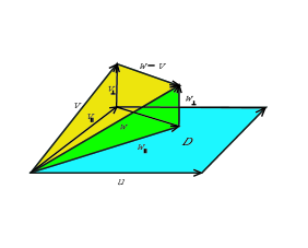
Figure 4: Passive boost in the spacetime plane of $D$.

Defining the active boost $L_{u}(x)=(\hat{w}_{\parallel}\hat{v}_{\parallel})^{\frac{1}{2}}x(\hat{v}_{\parallel}\hat{w}_{\parallel})^{\frac{1}{2}}$, we can easily check that it has the desired property that

$$L_{u}(v)=L_{u}(v_{\parallel}+v_{\perp})=\hat{w}_{\parallel}\hat{v}_{\parallel}v_{\parallel}+v_{\perp}=w_{\parallel}+w_{\perp}=w.$$

Thus, the active boost taking the unit timelike vector $\hat{v}_{\parallel}$ into the unit timelike vector $\hat{w}_{\parallel}$ is equivalent to the passive boost (19) in the plane of the spacetime bivector $D$. See Figure 4.

The above calculations show that each different system $u$ measures passive relative velocities between the systems $v$ and $w$ differently by a boost in the plane of the Minkowski bivector $D=(w-v)\wedge u$, whereas there is a unique active boost (8) that takes the system $v$ into $w$ in the plane of $v\wedge w$. The concept of a passive and active boost become equivalent when $u\wedge v\wedge w=0$, the case when ${\bf b}=\pm{\bf a}$.

Appendix: Matrix Representation

The algebraic rules satisfied by elements of $I\!\!\!G_{2}$ are completely compatible with the rules of matrix algebra and provide a geometric basis for $2\times 2$ matrices. By the spectral basis of $I\!\!\!G_{2}$ we mean

$$\pmatrix{1\cr{\bf e}_{1}}u_{+}\pmatrix{1&{\bf e}_{1}}=\pmatrix{u_{+}&{\bf e}_{1}u_{-}\cr{\bf e}_{1}u_{+}&u_{-}},$$ (34)

where $u_{\pm}=\frac{1}{2}(1\pm{\bf e}_{2})$ are mutually annihiliating idempotents, [12].

Noting that

$$\pmatrix{1&{\bf e}_{1}}u_{+}\pmatrix{1\cr{\bf e}_{1}}=u_{+}+{\bf e}_{1}u_{+}{\bf e}_{1}=u_{+}+u_{-}=1,$$

for $g=x+iy+v_{1}{\bf e}_{1}+v_{2}{\bf e}_{2}\in I\!\!\!G_{2}$, we find that

$$g=\pmatrix{1&{\bf e}_{1}}u_{+}\pmatrix{1\cr{\bf e}_{1}}g\pmatrix{1&{\bf e}_{1}}u_{+}\pmatrix{1\cr{\bf e}_{1}}$$

$$=\pmatrix{1&{\bf e}_{1}}u_{+}\pmatrix{g&g{\bf e}_{1}\cr{\bf e}_{1}g&{\bf e}_{1}g{\bf e}_{1}}u_{+}\pmatrix{1\cr{\bf e}_{1}}$$

$$=\pmatrix{1&{\bf e}_{1}}u_{+}\pmatrix{x+v_{2}&v_{1}-y\cr v_{1}+y&x-v_{2}}\pmatrix{1\cr{\bf e}_{1}}.$$

The real matrix $[g]:=\pmatrix{x+v_{2}&v_{1}-y\cr v_{1}+y&x-v_{2}}$ is called the matrix of $g$ with respect to the spectral basis (34).

By the inner automorphism or ${\bf e}_{1}$-conjugate $g^{{\bf e}_{1}}$ of $g\in I\!\!\!G_{3}$ with respect to the unit vector ${\bf e}_{1}$, we mean

$$g^{{\bf e}_{1}}:={\bf e}_{1}g{\bf e}_{1}.$$ (35)

We can now explicitly solve for the matrix $[g]$ of $g$.

$$\pmatrix{1\cr{\bf e}_{1}}g\pmatrix{1&{\bf e}_{1}}=\pmatrix{1&{\bf e}_{1}\cr{\bf e}_{1}&1}u_{+}[g]\pmatrix{1&{\bf e}_{1}\cr{\bf e}_{1}&1}$$

or

$$u_{+}\pmatrix{1\cr{\bf e}_{1}}g\pmatrix{1&{\bf e}_{1}}u_{+}=u_{+}\pmatrix{1&{\bf e}_{1}\cr{\bf e}_{1}&1}u_{+}[g]\pmatrix{1&{\bf e}_{1}\cr{\bf e}_{1}&1}u_{+}=u_{+}[g],$$

and taking the ${\bf e}_{1}$-conjugate of this equation gives

$$u_{-}\pmatrix{1\cr{\bf e}_{1}}g^{{\bf e}_{1}}\pmatrix{1&{\bf e}_{1}}u_{-}=u_{-}[g].$$

Adding the last two expressions gives the desired result that

$$[g]=u_{+}\pmatrix{g&g{\bf e}_{1}\cr{\bf e}_{1}g&{\bf e}_{1}g{\bf e}_{1}}u_{+}+u_{-}{\pmatrix{{\bf e}_{1}g{\bf e}_{1}&{\bf e}_{1}g\cr g{\bf e}_{1}&g}}u_{-}.$$

Of course, the geometric numbers of the spacetime algebra $I\!\!\!G_{1,2}$ also have a matrix representation. Since the unit pseudoscalar element $s=\gamma_{012}\in I\!\!\!G_{1,2}$ is in the center of the algebra, $s\in Z(I\!\!\!G_{1,2})$ and $s^{2}=-1$, it follows that a general element $f\in I\!\!\!G_{1,2}$ can be expressed as the complexification of the algebra $I\!\!\!G_{3}$. Thus, we write $f=g+sh$ for $g,h\in I\!\!\!G_{2}$. Then for $g=x_{1}+iy_{1}+a_{1}{\bf e}_{1}+a_{2}{\bf e}_{2}$ and $h=x_{2}+iy_{2}+b_{1}{\bf e}_{1}+b_{2}{\bf e}_{2}$, we have

$$[f]=[g+sh]=[g]+s[h]=\pmatrix{x_{1}+a_{2}&a_{1}-y_{1}\cr a_{1}+y_{1}&x_{1}-a_{2}}+s\pmatrix{x_{2}+b_{2}&b_{1}-y_{2}\cr b_{1}+y_{2}&x_{2}-b_{2}}.$$

The larger geometric algebra $I\!\!\!G_{1,2}$ has three involutions which are related to complex conjugation. The main involution is obtained by changing the sign of all vectors in $I\!\!\!G_{1,2}^{1}$. For $f=g+sh$, $f^{*}:=g-sh$. The main involution thus behaves as the complex conjugation of the pseudoscalar $s$. Reversion is obtained by reversing the order of the products of vectors in $I\!\!\!G_{1,2}^{1}$. For $f=g+sh$ given above, $f^{\dagger}=g^{\dagger}-sh^{\dagger}$ where $g^{\dagger}=x_{1}-iy_{1}-a_{1}{\bf e}_{1}-a_{2}{\bf e}_{2}$ and $h^{\dagger}=x_{2}-iy_{2}-b_{1}{\bf e}_{1}-b_{2}{\bf e}_{2}$ The third involution, called Clifford conjugation is obtained by combining the above two operations,

$$\widetilde{f}:=(f^{*})^{\dagger}={g^{*}}^{\dagger}-s{g^{*}}^{\dagger},$$ (36)

where ${g^{*}}^{\dagger}=x_{1}-iy_{1}-a_{1}{\bf e}_{1}-a_{2}{\bf e}_{2}$ and ${h^{*}}^{\dagger}=x_{2}-iy_{2}-b_{1}{\bf e}_{1}-b_{2}{\bf e}_{2}$ .

Finally, we note that the geometric algebra $I\!\!\!G_{1,2}$ is algebraically closed with $j=\gamma_{012}\in Z(I\!\!\!G_{1,2})$. This means that in dealing with the characteristic and minimal polynomials of the matrices which represent the elements of $I\!\!\!G_{1,2}$, we can always interpret complex zeros of these polynomials to be in the spacetime algebra $I\!\!\!G_{1,2}$.

References

[1] W.E. Baylis, G. Sobczyk, Relativity in Clifford’s geometric algebras of space and spacetime,
International Journal of Theoretical Physics, 43 (10) (2004) 1386-1399.
[2] W.K. Clifford, On the classification of geometric algebras; pp. 397-401 in R. Tucker (ed.):
Mathematical Papers by William Kingdon Clifford. Macmillan, London, 1882. (Reprinted by Chelsea, New York, 1968.)
[3] M.J. Crowe, A History of Vector Analysis: The Evolution of the Idea of a Vectorial System,
Dover 1994.
[4]
A. Einstein, H.A. Lorentz, H. Minkowski and H. Weyl, On the Electrodynamics of Moving Bodies,
in The Principle of Relativity.
Translated from “Zur Elektrodynamik bewegter Körper”, Annalen der Physik, 17, 1905, Dover
Publications, Inc. (1923).
[5] A. Hernández Pérez, Álgebra de vectores complejos en relatividad especial, Tesis
profesional de Licenciado en Física, Universidad de Las Américas - Puebla, 2002.
[6] D. Hestenes, Proper particle mechanics, Journal of Mathematical Physics15 (1974)
1768-1777.
[7] D. Hestenes, New Foundations for Classical Mechanics, 2nd Ed., Kluwer 1999.
[8] D. Hestenes, Spacetime physics with geometric algebra, American Journal of Physics71 (6) (2003).
[9] D. Hestenes and G. Sobczyk. Clifford Algebra to
Geometric Calculus: A Unified Language for Mathematics and Physics,
2nd edition, Kluwer 1992.
[10] P. Lounesto,
Clifford Algebras and Spinors, 2nd Ed.
Cambridge University Press, Cambridge, 2001.
[11] Z. Oziewicz, How do you add relative velocities?, in G.S. Pogosyan, L.E. Vicent and K.B. Wolf, eds.
Group Theoretical Methods in Physics, (Institute of Physics, Bristol 2005).
[12]
G. Sobczyk.
Clifford Geometric Algebras in Multilinear Algebra and Non-Euclidean Geometries.
Editor: Jim Byrnes, Computational Noncommutative Algebra and Applications:
NATO Science Series, 1–28, Kluwer 2004.
[13] G. Sobczyk, Hyperbolic Number Plane, The College Mathematics
Journal, Vol. 26, No. 4, pp.269-280, September 1995.
[14] G. Sobczyk, A Complex Gibbs-Heaviside Vector Algebra for Space-time, Acta Physica Polonica,
Vol. B12, No.5, 407-418, 1981.