On rational blow-downs in Heegaard-Floer homology

Abstract

Motivated by a result of L.P. Roberts on rational blow-downs in Heegaard-Floer homology, we study such operations along 3-manifolds that arise as branched double covers of $S^{3}$ along several non-alternating, slice knots.

1 Introduction

In 1993, R. Fintushel and R. Stern introduced the rational blow-down of smooth 4-manifolds, a surgical procedure consisting of removing the interior of a negative-definite simply connected smooth 4-manifold $C_{p}$ embedded in a closed smooth 4-manifold $X$ and replacing it with a rational homology ball. They also studied the effect of this process on both the Donaldson and the Seiberg-Witten invariants ([4]). Several years later, J. Park extended their results to more general configurations $C_{p,q}$, thus defining the generalized rational blow-down, and computed how the Seiberg-Witten invariants change under this operation ([19]). The first technique was used by Park in constructing an exotic smooth structure on $\mathbb{C}P^{2}\sharp 7\overline{\mathbb{C}P}^{2}$ ([20]), while the second was applied by Park, Stipsicz and Szabó in constructing exotic smooth structures on $\mathbb{C}P^{2}\sharp 6\overline{\mathbb{C}P}^{2}$ and $\mathbb{C}P^{2}\sharp 5\overline{\mathbb{C}P}^{2}$ ([23] and [21] respectively). More recently, in [24] and [5], D. Gay, A. Stipsicz, Z. Szabó and J. Wahl extended further the above procedures, this time along certain negative-definite plumbing trees, while in [22], L. Roberts studied the rational blow-down along the branched double cover $\Sigma(K)$ of $S^{3}$ along alternating, slice knots K in $S^{3}$ and its effect on the Ozsváth-Szabó 4-manifold invariant.

In this paper, we turn to study the rational blow-down operation along 3-manifolds that arise as branched double covers of $S^{3}$ along non-alternating, slice knots. We narrow our attention down to knots with up to ten crossings and then the knots $8_{20},9_{46},10_{129},10_{137},10_{140},10_{153}$ and $10_{155}$ are the only ones with the desired properties (see [10] and [2]). First, we study the mirrors of some of these knots, specifically $\overline{8_{20}},\overline{9_{46}},\overline{10_{137}}$ and $\overline{10_{140}}$, which are also non-alternating and slice. The branched double covers of $S^{3}$ along these (denoted by $Y_{1},Y_{2},Y_{3}$ and $Y_{4}$ respectively) bound negative-definite 4-manifolds as well as rational homology balls. The existence of such balls is guaranteed by the fact that the knots are slice, but we also find explicit descriptions of them using [3]. Using the results in [17] and [18], we show that the 3-manifolds $Y_{i}$, $i\in\{1,2,3,4\}$, are L-spaces and we then move on to write rational blow-down formulas along them, applying the results of Roberts in [22]. We note that the 3-manifolds $Y_{i}$, $i\in\{1,2,3,4\}$, along which we perform the rational blow-down do not belong in any of the categories $G_{rat}$, $W$, $N$, $M$, $A$, $B$, $C$ described in [24]. In the next to last section of the paper, we briefly discuss the cases of the branched double covers of $S^{3}$ along $10_{129},10_{153}$ and $10_{155}$ and in the last section, we present how the relationship between Heegaard-Floer homology and Khovanov homology can be used to draw some of the above conclusions over $\mathbb{Z}_{2}$ instead of $\mathbb{Q}$.

Acknowledgements: The author wishes to thank Z. Szabó for his guidance during the course of this work as well as J. Rasmussen and J. Greene for several helpful discussions.

2 Preliminaries

2.1 Weighted graphs

Let us start by introducing some terminology. Consider a graph $G$. The degree of a vertex $v$ of $G$, denoted $d(v)$, is the number of edges which contain $v$. If $G$ is equipped with an integer valued function $m$ on its vertices, then it is called a weighted graph and if $v$ is a vertex of such a graph, then $m(v)$ is called the multiplicity of $v$. A vertex $v$ of a weighted graph $G$ is called bad if

$$m(v)>-d(v).$$

A weighted graph $G$ gives rise to a 4-manifold $X(G)$ with boundary $Y(G)$. $X(G)$ is obtained as follows: On each vertex $v$ of $G$ consider a $D^{2}$-bundle over $S^{2}$ with Euler class $m(v)$. Whenever two vertices $v$ and $w$ are joined by an edge, ”plumb” the corresponding disk bundles, i.e. pick a small disk ($D_{v}$ and $D_{w}$) on each sphere so that the disk bundle over it is a product ($D_{v}\times D^{2}$ and $D_{w}\times D^{2}$) and then identify $D_{v}\times D^{2}$ with $D_{w}\times D^{2}$ using a map that preserves the product structures but interchanges the factors.

For $X(G)$ as above, $H_{2}(X(G);\mathbb{Z})$ is the lattice spanned by the vertices of G and if $[v]$ is the homology class corresponding to the vertex $v$, then the intersection form $Q_{X(G)}$ is given by: $Q_{X(G)}([v],[v])=m(v)$ and $Q_{X(G)}([v],[w])=1$ $(0)$ if the vertices $v$ and $w$ are (are not) connected by an edge.

A weighted graph $G$ is called negative-definite when it is a disjoint union of trees and $Q_{X(G)}$ is negative-definite.

2.2 The Ozsváth-Szabó 4-manifold invariant

We move on to briefly recalling the definition of the closed 4-manifold invariant $\Phi$ introduced in [15].

Consider $W$ a smooth, oriented, connected cobordism between two connected 3-manifolds $Y_{1}$ and $Y_{2}$ and $\mathfrak{s}$ a $spin^{c}$ structure on $W$. $W$ and $\mathfrak{s}$ induce maps $F_{W,\mathfrak{s}}^{+}$, $F_{W,\mathfrak{s}}^{-}$ and $F_{W,\mathfrak{s}}^{\infty}$ between $HF^{+}(Y_{1},\mathfrak{t}_{1})$ and $HF^{+}(Y_{2},\mathfrak{t}_{2})$ (respectively $HF^{-}(Y_{1},\mathfrak{t}_{1})$ and $HF^{-}(Y_{2},\mathfrak{t}_{2})$, $HF^{\infty}(Y_{1},\mathfrak{t}_{1})$ and $HF^{\infty}(Y_{2},\mathfrak{t}_{2})$), where $\mathfrak{t}_{i}=\mathfrak{s}|_{Y_{i}}$, $i\in\{1,2\}$. These maps are uniquely determined up to sign.

If $W$ is a closed 4-manifold, it can be punctured in two points and the resulting object can be viewed as a cobordism from $S^{3}$ to $S^{3}$. Under the additional condition that $b_{2}^{+}(W)>1$, this object can be further cut along some 3-manifold $Y$ and thus divided into two cobordisms $W_{1}$ and $W_{2}$ with $b_{2}^{+}(W_{i})>0$, $i\in\{1,2\}$, so that the map

$$Spin^{c}(W)\to Spin^{c}(W_{1})\times Spin^{c}(W_{2})$$

induced by restriction is injective. Then a ”mixed invariant”

$$F_{W,\mathfrak{s}}^{mix}:HF^{-}(Y_{1},\mathfrak{t_{1}})\to HF^{+}(Y_{2},\mathfrak{t_{2}})$$

can be defined by combining $F_{W_{1},\mathfrak{s}|_{W_{1}}}^{-}$ and $F_{W_{2},\mathfrak{s}|_{W_{2}}}^{+}$ in an appropriate way (using the identification $HF^{+}_{red}(Y,\mathfrak{s}|_{Y})\cong HF^{-}_{red}(Y,\mathfrak{s}|_{Y})$). This ”mixed invariant” gives rise to the invariant $\Phi_{W,\mathfrak{s}}$, which is a map

$$\Phi_{W,\mathfrak{s}}:\mathbb{Z}[U]\otimes\Lambda^{*}(H_{1}(W)/Tors)\to\mathbb{Z}/\pm 1$$

and is a smooth, oriented 4-manifold invariant.

2.3 The correction term $d(Y,\mathfrak{t})$

The 4-dimensional theory reviewed in the previous section has as a by-product an absolute rational lift to the relative $\mathbb{Z}$ grading on the Floer-homology groups of a 3-manifold $Y$ endowed with a torsion $spin^{c}$ structure. The correction term $d(Y,\mathfrak{t})$ that we discuss in the present section is an application of these absolute gradings.

In [12], the authors define a $\mathbb{Q}$-valued invariant $d(Y,\mathfrak{t})$ (also called the correction term $d(Y,\mathfrak{t})$) associated to an oriented rational homology 3-sphere Y equipped with a $spin^{c}$ structure $\mathfrak{t}$ as follows:

Definition 1.

$d(Y,\mathfrak{t})$ is the minimal grading ($\widetilde{gr}$) of any non-torsion element in the image of $HF^{\infty}(Y,\mathfrak{t})$ in $HF^{+}(Y,\mathfrak{t})$.

This is the Heegaard Floer homology analogue of the Frøyshov invariant in Seiberg-Witten theory.

In the same paper it is proven that if $Y$ and $\mathfrak{t}$ are as above and $X$ is a smooth, negative-definite 4-manifold with $\partial X=Y$, then $\forall$ $\mathfrak{s}\in Spin^{c}(X)$ with $\mathfrak{s}|_{Y}=\mathfrak{t}$

$$c_{1}(\mathfrak{s})^{2}+rk(H^{2}(X;\mathbb{Z}))\leq 4d(Y,\mathfrak{t})$$

In addition, in [17], Corollary 1.5, it is proven that for negative-definite graphs G with at most two bad vertices

$$d(Y(G)),\mathfrak{t})=max_{\{K\in Char_{\mathfrak{t}}((G))\}}\frac{K^{2}+|G|}{4}$$ (1)

where $Char_{\mathfrak{t}}(G)$ denotes the set of characteristic vectors for $X(G)$ which are first Chern classes of $spin^{c}$ structures whose restriction to the boundary is $\mathfrak{t}$ and $K^{2}$ is computed using $Q_{X(G)}^{-1}$.

3 Rational blow-down along $Y_{1}=\Sigma(\overline{8_{20}})$

Denote the branched double cover of $S^{3}$ along $\overline{8_{20}}$ by $Y_{1}=\Sigma(\overline{8_{20}})$.

3.1 A negative-definite 4-manifold $W_{1}$ with $\partial(W_{1})=Y_{1}$.

Consider the knot $\overline{8_{20}}$ and following [18] construct a checkerboard coloring of the plane (see Figure 1).

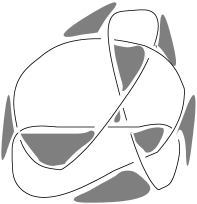
Figure 1: A checkerboard coloring for $\overline{8_{20}}$

Associate 1-handles to the black regions but one (the outer region in Figure 1, without loss of generality) and at each crossing add a $\pm 1$ framed 2-handle to an unknot looping through the two 1-handles using the sign convention of Figure 2.

Figure 2: Sign convention

This process gives a 4-manifold $W_{1}$ with boundary $\Sigma(\overline{8_{20}})$. After appropriate cancelations of 1-handles by 2-handles (see section 5.4 of [6] for more details), the 4-manifold described above can be represented by the plumbing tree below

3.2 $Y_{1}$ is an L-space

In this subsection, we will exhibit that $Y_{1}$ is an L-space. The notion of an L-space is a generalization of that of a lens space. The precise definition is as follows ([16]):

Definition 2.

A closed 3-manifold Y is called an L-space if $H_{1}(Y;\mathbb{Q})=0$ and $\widehat{HF}(Y)$ is a free abelian group with rank equal to $|H_{1}(Y;\mathbb{Z})|$, the number of elements in $H_{1}(Y;\mathbb{Z})$.

$\widehat{HF}(Y)$ is the 3-manifold invariant defined in [13].

$Y_{1}$ is a rational homology sphere ($\mathbb{Q}HS^{3}$), as is the branched double cover of $S^{3}$ along any knot K, denoted from now on as $\Sigma(K)$. This is true because $|H_{1}(\Sigma(K);\mathbb{Z})|=|\Delta_{K}(-1)|=det(K)$ finite.

To prove that $Y_{1}$ is an L-space over $\mathbb{Q}$, we first need to introduce the notion of a quasi-alternating link, as defined in [18].

Definition 3.

The set $Q$ of quasi alternating links is the smallest set of links which satisfies the following properties:

1. the unknot is in $Q$

2. the set $Q$ is closed under the following operation. Suppose $L$ is a link which admits a projection with a crossing with the following properties:

   • both resolutions $L_{0},L_{1}\in Q$ (see Figure 3)

   • $det(L_{0}),det(L_{1})\neq 0$

   • $det(L)=det(L_{0})+det(L_{1})$

   then $L\in Q$.

2pt $L$ at 22 0 $L_{0}$ at 96 0 $L_{1}$ at 168 0

Figure 3: The 0-and 1-resolutions of a link L at one of its crossings as above are obtained by replacing this crossing with the simplified pictures shown in the figure.

Proposition 1.

$\overline{8_{20}}$ is a quasi-alternating knot.

Proof.

Consider a projection of $\overline{8_{20}}$ like the one in Figure 1 and resolve the left topmost crossing. It is easy to see that the 1-resolution yields the unknot and the 0-resolution yields the link shown in Figure 4, call it L.

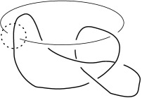
Figure 4: The 0-resolution of $8_{20}$ at it’s left topmost crossing.

Using the skein relationship $\Delta_{L_{+}}(x)-\Delta_{L_{-}}(x)+(x^{-\frac{1}{2}}-x^{\frac{1}{2}})\Delta_{L_{0}}(x)=0$ (Figure 5 conveys the meaning of $L_{+},L_{-}$ and $L_{0}$) satisfied by the Conway normalized Alexander polynomial (see [9]), one can compute that $\Delta_{L}(x)=x^{-\frac{3}{2}}-3x^{-\frac{1}{2}}+3x^{\frac{1}{2}}-x^{\frac{3}{2}}$ and $det(L)=|\Delta_{L}(-1)|=8$.

2pt $L_{+}$ at 22 -4 $L_{-}$ at 102 -4 $L_{0}$ at 185 -4

Figure 5: $L_{+},L_{-}$ and $L_{0}$ in the skein relationship for the Alexander polynomial

Thus, it remains to prove that L is in it’s turn a quasi-alternating link. To this end, we resolve the marked crossing in Figure 4 and we get the unknot as the 1-resolution and the knot $\overline{5_{2}}$ as the 0-resolution. The result folows, since $\overline{5_{2}}$ is alternating, thus quasi-alternating (See Lemma 3.2 of [18]), and $det(\overline{5_{2}})=|\Delta_{\overline{5_{2}}}(-1)|=|\Delta_{5_{2}}(-1)|=|2(-1)^{-1}-3+2(-1)|=7$.

∎

Corollary 1.

$Y_{1}=\Sigma(\overline{8_{20}})$ is an L-space

Proof.

Making use of a result in [18] that states that if $L$ is a quasi-alternating link, then $\Sigma(L)$ is an L-space, Proposition 1 implies that $Y_{1}=\Sigma(\overline{8_{20}})$ is an L-space. ∎

3.3 $Y_{1}$ bounds a rational homology ball $B_{1}$

To see this, it suffices to notice that $\overline{8_{20}}$ is slice and the branched cover of $B^{4}$ along the slice disk is a rational homology ball. We mention here that whether a knot is slice or not can be read off from its smooth four genus, which has been computed for all knots up to ten crossings and is listed on the corresponding knot tables. For the specific case of the knot $8_{20}$ that we are studying here, the interested reader is refered to page 86 of [9] for a concrete description of the slice disc.

In fact, $Y_{1}$ is one of the manifolds listed in [3], it is the manifold $(2,3,3;9)$ in category (5) with p=3 and s=-1. Thus, we can explicitly describe a 2-handle addition to $Y_{1}\times I$ along a circle in $Y_{1}\times 1$ that leads to a manifold with boundary $Y_{1}\bigcup S^{1}\times S^{2}$ and eventually, after attaching a 3- and a 4-handle, to a rational homology ball $B_{1}$ with boundary $Y_{1}$. We proceed to do so.

First note that $Y_{1}$ can be alternatively represented as in Figure 6.

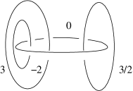
Figure 6: An alternative description of $Y_{1}$

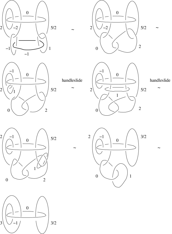
Figure 14: 2-handle addition for $Y_{1}$

Then, there is a 2-handle addition depicted in the first part of Figure 14 at the end of the paper that has as end product the last manifold of this figure, which, according to the Lemma in page 26 of [3], is homeomorphic to $S^{1}\times S^{2}$.

3.4 Blow-down formula

We will call our graph $G_{1}$ and label its vertices as shown below

Note that $G_{1}$ has only one bad vertex and that is $v_{2}$ with $-2=m(v_{2})>-d(v_{2})=-3$.

First, we will make use of the calculations of the Heegaard Floer homology groups for 3-manifolds obtained by plumbings of spheres specified by certain graphs carried out in section 3 of [17]. It is easy to check that of the 48 characteristic vectors $K_{0}\in\{0,2\}\times\{0,2\}\times\{0,2\}\times\{0,2\}\times\{-1,1,3\}$, after applying the algorithm described in section 3 of [17], only 9 initiate a path ending at a vector $L$ satisfying

$$-2\leq\langle L,v_{i}\rangle\leq 0\mbox{ }\forall\mbox{ }i\in\{1,2,3,4\}$$ (2)

$$-3\leq\langle L,v_{5}\rangle\leq 1$$ (3)

These are the following: $(0,0,0,0,\pm 1),(2,0,0,0,\pm 1),(0,0,0,2,\pm 1),$
$(0,0,0,0,3),(0,0,2,0,-1)$ and $(0,2,0,0,-1)$.

Remark 1.

This, together with the fact that $|H_{1}(Y_{1})|=9$, provides an alternative proof of the fact that $Y_{1}$ is an L-space.

Next, we need to check which of the above 9 vectors representing $spin^{c}$ structures on $Y_{1}$ extend to the rational homology ball. Figure 7 illustrates the first few steps of computing the enhanced intersection form after the 2-handle addition that we presented at the end of section 3.3. We leave it as an exercise to the reader to carry out the next few steps and we only record here the outcome of this process:

$$A_{1}=\begin{pmatrix}-2&1&0&0&0&0\\ 1&-2&1&0&1&0\\ 0&1&-2&1&0&0\\ 0&0&1&-2&0&-1\\ 0&1&0&0&-3&-2\\ 0&0&0&-1&-2&-4\end{pmatrix}$$

with $Ker(A_{1})=<(-1,-2,-\frac{5}{3},-\frac{4}{3},-\frac{4}{3},1)>.$ The $spin^{c}$ structures that extend are represented by vectors that are orthogonal to the kernel of the enhanced intesection form, that is satisfy

$$(a_{1},a_{2},a_{3},a_{4},a_{5},a_{6})(-1,-2,-\frac{5}{3},-\frac{4}{3},-\frac{4}{3},1)=0$$ (4)

It is easy to see that only 3 of these vectors, specifically (0,0,0,0,3),(0,0,0,2,1) and (0,0,2,0,-1), satisfy the equation

$$2a_{3}+a_{4}+a_{5}\equiv 0(mod3)$$ (5)

and thus can be extended to the rational homology ball.

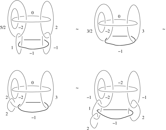
Figure 7: Computing the enhanced intersection form

Proposition 2.

Let $X_{W_{1}}$ be a closed, oriented, smooth 4-manifold with $b_{2}^{+}(X_{W_{1}})>1$ containing $W_{1}$ and let $\mathfrak{s}_{i},$ $i\in\{1,2,3\}$, $spin^{c}$ structures on $X_{W_{1}}$ that restrict to $W_{1}$ to give the three $spin^{c}$ structures listed above. Then, for any $\phi\in Diff^{+}(Y_{1})$ the 4-manifold $X_{B_{1}}=(X_{W_{1}}-W_{1})\bigcup_{\phi}B_{1}$ has $spin^{c}$ structures $\mathfrak{s^{\prime}}_{i}$, $i\in\{1,2,3\}$, for which

$\Phi_{(X_{B_{1}},\mathfrak{s^{\prime}}_{i})}=\pm\Phi_{(X_{W_{1}},\mathfrak{s}_{i})}$

Proof.

Call $\mathfrak{t}_{i}=\mathfrak{s}_{i}|_{Y_{1}}$. We will apply Theorem 2 of [22], so we only need to check that $Y_{1}$ satisfies the three conditions listed there. We have already seen that $Y_{1}$ is a rational homology sphere, so it remains to check the last two conditions. For the second condition, recall that there is a long exact sequence

$$...\rightarrow HF^{-}(Y_{1},\mathfrak{t}_{i})\xrightarrow{\text{i}}HF^{\infty}(Y_{1},\mathfrak{t}_{i})\xrightarrow{\text{$\pi$}}HF^{+}(Y_{1},\mathfrak{t}_{i})\xrightarrow{\text{$\delta$}}...$$

and that the 3-manifold invariant $HF^{+}_{red}(Y_{1},\mathfrak{t}_{i})$ is defined as $HF^{+}_{red}(Y_{1},\mathfrak{t}_{i})=Coker(\pi)=HF^{+}(Y_{1},\mathfrak{t}_{i})/Im\pi$. But $Y_{1}$ is an L-space, so the map $\delta$ is trivial, $Im\pi=Ker\delta=HF^{+}(Y_{1},\mathfrak{t}_{i})$ and $HF^{+}_{red}(Y_{1},\mathfrak{t}_{i})=0$. Hence the second condition of the theorem holds as well. Finally, the third condition requires $W_{i}$ to be a sleek negative-definite 4-manifold. This is true according to the results in [17], given that $G_{1}$ is a negative-definite graph with only one bad vertex. ∎

3.5 Using $d(Y,\mathfrak{t})$ to study the rational blow-down operation

At this point, we present a different approach to studying which of the $spin^{c}$ structures extend to the rational homology ball. The advantage of this approach is that it does not require a concrete description of the rational homology ball.

Fix a $spin^{c}$ structure $\mathfrak{t}$ over $Y_{1}$. Then

$$d(Y_{1},\mathfrak{t})=max_{\{K\in Char_{\mathfrak{t}}(G_{1})\}}\frac{K^{2}+5}{4}$$ (6)

since the graph $G_{1}$ that we are presently studying has only one bad vertex. By Proposition 3.2 of [17] the maximum is always achieved among the characteristic vectors in $Char_{\mathfrak{t}}(G_{1})$ which have coordinates in $\{0,2\}\times\{0,2\}\times\{0,2\}\times\{0,2\}\times\{-1,1,3\}$ and initiate paths with final vectors satisfying the equations (2) and (3).

Furthermore, if a $spin^{c}$ structure $\mathfrak{t}$ extends across a rational homology ball, then $d(Y_{1},\mathfrak{t})=0$. This follows from the more general statement proven in Proposition 9.9 of [12] that if $(Y_{1},\mathfrak{t}_{1})$ and $(Y_{2},\mathfrak{t}_{2})$ are rational homology cobordant rational homology 3-spheres equipped with $spin^{c}$ structures, then $d(Y_{1},\mathfrak{t}_{1})=d(Y_{2},\mathfrak{t}_{2})$.

We compute the square of the nine vectors above and only $(0,0,0,0,3)$, $(0,0,0,2,1)$ and $(0,0,2,0,-1)$ have square equal to -5. Therefore these give the only candidates for $spin^{c}$ structures that extend.

Moreover, we were already expecting precisely $3=\sqrt{9}=\sqrt{|H_{1}(Y_{1};\mathbb{Z})|}$ $spin^{c}$ structures to extend, according to the arguments presented in Lemma 2 of [22]. We restate this here and then use it to justify our claim.

Lemma 1.

$Y$ is a rational homology 3-sphere and $h=|H_{1}(Y;\mathbb{Z})|$. $Y$ bounds $X$ and $s=|det(Q_{X})|$, $Q_{X}$ denoting the intersection form of $X$. Then $h=st^{2}$ where $t$ is the order of the image of the torsion of $H^{2}(X;\mathbb{Z})$ in $H^{2}(Y;\mathbb{Z})$ (and $st$ is the order of the image of $H^{2}(X;\mathbb{Z})$ in $H^{2}(Y;\mathbb{Z})$).

Applying this for $X=B_{1}$ and $Y=Y_{1}$ and setting $s=1$ since $b_{2}(B_{1})=0$ gives that $9=|H_{1}(Y_{1};\mathbb{Z})|=t^{2}$ and so $t=3$, i.e. the order of the image of the torsion of $H^{2}(B_{1};\mathbb{Z})$ in $H^{2}(Y_{1};\mathbb{Z})$ is 3.

The arguments in the preceding two paragraphs verify the answer we got using the enhanced intersection form.

4 Rational blow-down along $Y_{2}=\Sigma(\overline{9_{46}})$

Denote the branched double cover of $S^{3}$ along $\overline{9_{46}}$ by $Y_{2}=\Sigma(\overline{9_{46}})$. Following a process analogous to that of subsection 1.1, we construct a negative-definite 4-manifold $W_{2}$ with $\partial(W_{2})=Y_{2}$. This is depicted below:

Using the algorithm presented in subsection 1.4, we compute that only 9 of the 96 characteristic vectors $K_{0}\in\{0,2\}\times\{0,2\}\times\{0,2\}\times\{0,2\}\times\{0,2\}\times\{-1,1,3\}$ initiate paths that terminate in a vector $L$ satisfying

$$-2\leq\langle L,v_{i}\rangle\leq 0\mbox{ }\forall\mbox{ }i\in\{1,2,3,4,5\}$$ (7)

$$-3\leq\langle L,v_{6}\rangle\leq 1$$ (8)

where $v_{1},v_{2},v_{3},v_{4},v_{5}$ are the vertices with multiplicity -2 of the graph above enumerated from left to right and $v_{6}$ is the bottom vertex of the same graph. These vectors are $(0,0,0,0,0,\pm 1),$ $(0,0,0,0,0,3),$ $(0,0,0,0,2,-1)$, $(2,0,0,0,0,-1),$ $(0,0,0,2,0,-1),$ $(0,2,0,0,0,-1),$ $(2,0,0,0,0,1),$ $(0,0,0,0,2,1)$. Since $|H_{1}(Y_{2};\mathbb{Z})|=det(9_{46})=9$, we deduce that $Y_{2}$ is an L-space.

Remark 2.

In a recent paper ([11]), C. Manolescu and P. Ozsváth show that all but 2 ($8_{19}$ and $9_{42}$)of the 85 prime knots with up to nine crossings are quasi-alternating, which implies that the corresponding branched double covers of $S^{3}$ are L-spaces.

Lastly, we know that $Y_{2}$ bounds a rational homology ball since $\overline{9_{46}}$ is slice and thus we can move on to write a blow-down formula along $Y_{2}$.

To this end, we compute the squares of the above 9 vectors. It turns out that 5 of them have square -6, thus giving $d=0$ for the corresponding $spin^{c}$ structures. These are the vectors $3v_{6}=(0,0,0,0,0,3)$, $2v_{4}-v_{6}=(0,0,0,2,0,-1)$, $2v_{5}-v_{6}=(0,0,0,0,2,1)$, $2v_{2}-v_{6}=(0,2,0,0,0,-1)$ and $2v_{1}-v_{6}=(2,0,0,0,0,1)$. This comes as no surprise, if we take into account the symmetry of $Y_{2}$ obvious from the plumbing diagram of $W_{2}$ above (consider the triads $\{3v_{6},2v_{4}-v_{6},2v_{5}-v_{6}\}$ and $\{3v_{6},2v_{2}-v_{6},2v_{1}-v_{6}\}$) and for these $spin^{c}$ structures, one can write down a blow-down formula analogous to that of Proposition 2.

Remark 3.

An alternative description of $Y_{2}$ is given in Figure 8.

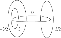
Figure 8: An alternative description of $Y_{2}$

Using this, we find that $Y_{2}$ is the manifold $(3,3,3;9)$ of category (3) of the main theorem in [3] with $p=q=3$ and $s=0$ and we can compute that the 2-handle addition shown in Figure 9 yields one way to construct a rational homology ball bounded by $Y_{2}$.

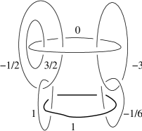
Figure 9: 2-handle addition for $Y_{2}$

However, we will not need to make use of this in order to write down the blow-down formula in this case.

5 Rational blow-down along $Y_{3}=\Sigma(\overline{10_{137}})$

$W_{3}$ below is a negative-definite 4-manifold with $\partial W_{3}=Y_{3}$.

$Y_{3}$ is an L-space, since $|H_{1}(Y_{3};\mathbb{Z})|=det(10_{137})=25$ and out of the 144 characteristic vectors $K_{0}\in\{0,2\}\times\{0,2\}\times\{-1,1,3\}\times\{0,2\}\times\{0,2\}\times\{-1,1,3\}$ exactly 25 initiate paths ending in a vector L satisfying

$$-2\leq\langle L,v_{i}\rangle\leq 0\mbox{ }\forall\mbox{ }i\in\{1,2,4,5\}$$ (9)

$$-3\leq\langle L,v_{i}\rangle\leq 1\mbox{ }\forall\mbox{ }i\in\{3,6\}$$ (10)

with $v_{1}$, $v_{2}$, $v_{3}$, $v_{4}$ the vertices on the horizontal part of the graph from left to right and $v_{5}$, $v_{6}$ the remaining two vertices on the vertical part from top to bottom. We list these vectors here:
$(0,0,\pm 1,0,0,\pm 1)$, $(0,0,\pm 1,0,0,3)$, $(0,0,\pm 1,2,0,\pm 1)$, $(0,0,-1,2,0,3)$,
$(0,0,-1,0,2,\pm 1)$, $(0,0,1,2,0,-1)$, $(0,2,-1,0,0,\pm 1)$, $(2,0,\pm 1,0,0\pm 1)$,
$(2,0,-1,2,0,\pm 1)$, $(0,0,3,0,0,\pm 1)$, $(0,0,-1,2,2,-1)$.

Finally, $\overline{10_{137}}$ is slice and therefore $Y_{3}$ bounds a rational homology ball.

We compute the squares of the above listed vectors and it turns out that precisely 5 ($=\sqrt{25}$) of them have square equal to -6. These are $(0,0,1,0,0,3),$ $(0,0,-1,0,2,1),$ $(0,0,1,2,0,1),$ $(0,0,3,0,0,-1),$ $(0,0,-1,2,2,-1)$ and according to arguments presented in section 3.5, these give the $spin^{c}$ structures that extend to the rational homology ball.

For them, we can write a blow-down formula similar to that of Proposition 2.

Remark 4.

$Y_{3}$ is also among the manifolds listed in [3], in particular it is the manifold (2,5,5;25) in category (5) with p=5 and s=-1.

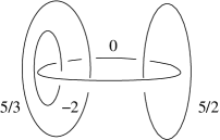
Figure 10: The manifold $Y_{3}$

Figures 10 and 11 present the manifold $Y_{3}$ and a surgery that leads to the construction of a rational homology ball $B_{3}$ with $\partial(B_{3})=Y_{3}$ respectively.

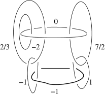
Figure 11: 2-handle addition for $Y_{3}$

The enhanced intersection form in this case is given by:

$$A_{3}=\begin{pmatrix}-2&1&0&0&0&0&0\\ 1&-2&1&0&1&0&0\\ 0&1&-3&1&0&0&-1\\ 0&0&1&-2&0&0&-1\\ 0&1&0&0&-2&1&0\\ 0&0&0&0&1&-3&-2\\ 0&0&-1&-1&0&-2&-5\end{pmatrix}$$

with $Ker(A_{3})=<(-1,-2,-\frac{7}{5},-\frac{6}{5},-\frac{8}{5},-\frac{6}{5},1)>.$

From our list of 25 vectors satisfying (9) and (10) only 5 are orthogonal to $Ker(A_{3})$, the same 5 that have square equal to -6. This verifies the conclusions of the first part of our exposition on blowing-down along $Y_{3}$.

6 Rational blow-down along $Y_{4}=\Sigma(\overline{10_{140}})$

A negative-definite 4-manifold $W_{4}$ with $\partial W_{4}=Y_{4}$ is depicted in the next picture.

Label the vertices of the graph above as $v_{1},...,v_{7}$ starting with those with multiplicity -2 from left to right and finishing at the vertex with multiplicity -3. Among the 192 characteristic vectors $K_{0}\in\{0,2\}\times\{0,2\}\times\{0,2\}\times\{0,2\}\times\{0,2\}\times\{0,2\}\times\{-1,1,3\}$ 9 initiate paths ending in a vector L satisfying

$$-2\leq\langle L,v_{i}\rangle\leq 0\mbox{ }\forall\mbox{ }i\in\{1,...,6\}$$ (11)

$$-3\leq\langle L,v_{7}\rangle\leq 1$$ (12)

They are the vectors $(0,0,0,0,0,0,\pm 1)$, $(0,0,0,0,0,0,3)$, $(2,0,0,0,0,0,\pm 1)$, $(0,2,0,0,0,0,-1)$, $(0,0,0,0,2,0,-1)$, $(0,0,0,0,0,2,\pm 1)$. Since $|H_{1}(Y_{4};\mathbb{Z})|=det(10_{140})=9$, we conclude that $Y_{4}$ is an L-space.

Once again, this particularly nice structure of our 3-manifold $Y$ allows us to write a blow-down formula along it. ($\overline{10_{140}}$ being slice guarantees the existence of a $\mathbb{Q}HB^{4}$ with boundary $Y_{4}$.) To study which of the $spin^{c}$ structures on $Y_{4}$ extend to the $\mathbb{Q}HB^{4}$, we can compute $d$ for the 9 vectors on our list. $(0,0,0,0,0,0,3)$, $(2,0,0,0,0,0,1)$, $(0,2,0,0,0,0,-1)$ are the only ones with square equal to -7 and for the three $spin^{c}$ structures corresponding to them we can write the blow-down formula.

Remark 5.

$Y_{4}$ is the manifold (3,3,4;9) in the notation of Casson and Harer in [3]. It belongs to category (3) with p=3, q=4 and s=0. Figures 12 and 13 suggest how to construct a rational homology ball $B_{4}$ with $\partial B_{4}=Y_{4}$.

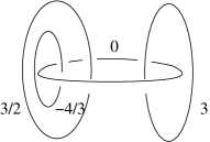
Figure 12: The manifold $Y_{4}$

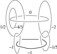
Figure 13: 2-handle addition for $Y_{4}$

7 The knots $10_{129}$, $10_{153}$ and $10_{155}$.

The cases of the remaining three knots among the seven listed in the introduction (i.e. $10_{129}$, $10_{153}$ and $10_{155}$) are still to be studied, since the techniques used in this paper are inconclusive for these examples.

8 Addendum

In this last section, we discuss some conclusions regarding our constructions that can be drawn from the relationship between Heegaard-Floer homology and Khovanov homology.

8.1 Background in Khovanov homology

In [7], M. Khovanov presented an algorithm that computes an invariant of knots and links. Given a link $L$, this invariant is a bigraded homology theory $Kh(L)$ (strictly speaking cohomology theory, since the boundary map increases the homological grading by 1) that categorifies the Jones polynomial, in the sense that its graded Euler characteristic is the unnormalized Jones polynomial of the link:

$$\sum_{i,j\in\mathbb{Z}}(-1)^{i}q^{j}dim(Kh^{i,j}(L))=\widehat{J}(L).$$

We confine our presentation here to mentioning that the starting point in defining $Kh(L)$ is to use the state-sum expression for the unnormalized Jones polynomial $\widehat{J}$.

In addition to the homology groups $Kh^{i,j}(L)$, reduced homology groups $\widetilde{Kh}^{i,j}(L)$ can be defined by tensoring the original chain complex with $Q$, where $Q=A/XA$ is the one-dimensional representation of the base ring $A$, to obtain a reduced chain complex. The Euler characteristic of $\widetilde{Kh}$ is the Jones polynomial:

$$\sum_{i,j\in\mathbb{Z}}(-1)^{i}q^{j}dim(\widetilde{Kh}^{i,j}(L))=J(L).$$

For our purposes, we are interested in the category of H-thin knots:

Definition 4.

A knot K is called homologically thin or H-thin if its nontrivial groups $Kh^{i,j}(K)$ lie on two adjacent diagonals. By a diagonal we mean a line $2i-j=k$, for some $k$.

As it turns out ([1]), all but 12 of the 249 knots with at most 10 crossings are H-thin and for these knots the homology groups are supported on the diagonals $j-2i=\sigma\pm 1$, where $\sigma$ denotes the signature of the knot. Moreover, both the Jones and the Alexander polynomials are alternating and the groups $\widetilde{Kh}^{i,j}(L)$ lie on one diagonal. Consequently, for these knots the dimensions of $\widetilde{Kh}^{i,j}(L)$ are given by the absolute values of the coefficients of $J(L)$ ([8]).

8.2 The conclusions

We make the following observations concerning the mirror image $\overline{K}$ of a slice, H-thin knot $K$. According to [7], for $K$ oriented knot and integers $i,j$, there are equalities of isomorphism classes of abelian groups

$$Kh^{i,j}(\overline{K})\otimes\mathbb{Q}=Kh^{-i,-j}(K)\otimes\mathbb{Q}.$$ (13)

$$Tor(Kh^{i,j}(\overline{K}))=Tor(Kh^{1-i,-j}(K))$$ (14)

We saw in the previous section that for an H-thin knot $K$ the Khovanov homology is supported in the diagonals $j-2i=\sigma+1$ and $j-2i=\sigma-1$. If $K$ is also slice, then it has signature $\sigma=0$ and so the Khovanov homology of an H-thin and slice knot $K$ is supported in the diagonals $j-2i=1$ and $j-2i=-1$. From equation (13) it follows that the non-torsion part of $Kh(\overline{K})$ is also supported in the same diagonals. From equation (14) it follows that the torsion part of $Kh(K)$ in the $j-2i=-1$ diagonal gives a torsion part in the same diagonal for $Kh(\overline{K})$ while the torsion part of $Kh(K)$ in the $j-2i=1$ diagonal gives a torsion part in the line $j-2i=-3$ for $Kh(\overline{K})$.

For our examples of knots, that is $8_{20},$ $9_{46},$ $10_{137}$ and $10_{140}$, we read off from the knot table ([2]) that these knots are H-thin and that torsion appears only on the $j-2i=-1$ diagonal and thus we can conclude that the mirror knots $\overline{8_{20}},$ $\overline{9_{46}},$ $\overline{10_{137}}$ and $\overline{10_{140}}$ are also H-thin.

Proposition 3.

$Y_{i}$ is an L-space over $\mathbb{Z}_{2}$, $i\in\{1,2,3,4\}$.

Proof.

We start by studying $Y_{1}=\Sigma(\overline{8_{20}})$. We know that

$$9=det(\overline{8_{20}})=|H_{1}(\Sigma(\overline{8_{20}}))|=|H^{2}(\Sigma(\overline{8_{20}}))|.$$

Also,

$$|H^{2}(\Sigma(\overline{8_{20}}))|=|Spin^{c}(\Sigma(\overline{8_{20}}))|$$

because there is an isomorphism between $H^{2}(\Sigma(\overline{8_{20}}))$ and $Spin^{c}(\Sigma(\overline{8_{20}}))$ (see [6] for a discussion on this) and

$$|Spin^{c}(\Sigma(\overline{8_{20}}))|\leq rk(\widehat{HF}(\Sigma(\overline{8_{20}})))$$

because $b_{1}(\Sigma(\overline{8_{20}}))=0$ and $|Spin^{c}(\Sigma(\overline{8_{20}}))|$ gives the Euler characteristic of $\widehat{HF}(\Sigma(\overline{8_{20}}))$ according to Proposition 5.1 of [14]. Furthermore,

$$rk(\widehat{HF}(\Sigma(\overline{8_{20}})))\leq rk(\widetilde{Kh}(\overline{8_{20}}))$$

(where both ranks refer to homology with $\mathbb{Z}_{2}$ coefficients) as there exists a spectral sequence with $E^{2}$ term $\widetilde{Kh}(8_{20})$ with $\mathbb{Z}_{2}$ coefficients and $E^{\infty}$ term $\widehat{HF}(\Sigma(\overline{8_{20}});\mathbb{Z}_{2})$ ([18]) and $rk(\widetilde{Kh}(\overline{8_{20}}))=rk(\widetilde{Kh}(8_{20}))$. Lastly, according to Corollary 2 of [8] the dimensions of the reduced homology groups for an H-thin knot are given by the absolute values of the coefficients of it’s Jones polynomial and

$$J(8_{20})=-q+2-q^{-1}+2q^{-2}-q^{-3}+q^{-4}-q^{-5}$$

giving that

$$rk(\widetilde{Kh}(\overline{8_{20}}))=rk(\widetilde{Kh}(8_{20}))=9.$$

Combining all the above relations in the order presented, we get that

$$rk(\widehat{HF}(\Sigma(\overline{8_{20}});\mathbb{Z}_{2}))=|Spin^{c}(\Sigma(\overline{8_{20}}))|=9$$

which translates to the fact that $\Sigma(\overline{8_{20}})$ is an L-space over $\mathbb{Z}_{2}$.

Similarly, $det(9_{46})=9=rk(\widetilde{Kh}(9_{46}))$, $det(10_{137})=25=rk(\widetilde{Kh}(10_{137}))$, $det(10_{140})=9=rk(\widetilde{Kh}(10_{140}))$ and the analogous conclusions can be drawn for these examples. ∎

References

- [1] D. Bar-Natan, On Khovanov’s categorification of the Jones polynomial, Algebraic and Geometric Topology 2-16 (2002) 337-370, arXiv:math.QA/0201043
-
[2]
D. Bar-Natan, S. Morrison, The Knot Atlas:
http://katlas.math.toronto.edu/wiki/ - [3] A. Casson, J. Harer, Some homology lens spaces which bound rational homology balls, Pacific Journal of Mathematics, Vol. 96, No. 1, 1981
- [4] R. Fintushel, R. Stern, Rational blowdowns of smooth 4-manifolds, J. Differential Geometry, 46 (1997), 181-235
- [5] D. Gay, A. Stipsicz, Symplectic rational blow-down along Seifert-fibered 3-manifolds, arXiv:math.SG/0703370 v1
- [6] R. Gompf, A. Stipcisz, 4-maifolds and Kirby Calculus, Graduate Studies in Mathematics, Volume 20, AMS
- [7] M. Khovanov, A categorification of the Jones polynomial, Duke Math. J. 101 (2000), no. 3, 359–426, arXiv:math.QA/9908171 v2
- [8] M. Khovanov, Patterns in knot cohomology I, Experimental mathematics 12 (2003), no. 3, 365–374, arXiv:math.QA/0201306 v1
- [9] R. Lickorish, An Introduction to Knot Theory, Springer
-
[10]
C. Livingston, Table of Knot Invariants:
http://www.indiana.edu/knotinfo/ - [11] C. Manolescu, P. Ozsváth, On the Khovanov and knot Floer homologies of quasi-alternating links, arXiv:0708.3249v1
- [12] P. Ozsváth, Z. Szabó, Absolutely graded Floer homologies and intersections forms for four-manifolds with boundary, Advances in Mathematics 173 (2003) 179-261
- [13] P. Ozsváth, Z. Szabó, Holomorphic disks and topological invariants for closed 3-manifolds, Annals of Mathematics 159 (2004), no. 3, 1027-1158.
- [14] P. Ozsváth, Z. Szabó, Holomorphic disks and three-manifolds invariants: Properties and applications, Annals of Mathematics 159 (2004) no. 3, 1159-1245.
- [15] P. Ozsváth, Z. Szabó, Holomorphic triangles and invariants for smooth four-manifolds, arXiv:math.GT/0401426 v2
- [16] P. Ozsváth, Z. Szabó, On Knot Floer homology and lens space surgeries, Topology 44 (2005), no. 6, 1281-1300, arXiv:math.GT/0303017 v2
- [17] P. Ozsváth, Z. Szabó, On the Floer homology of plumbed three-manifolds, Geometry and Topology, Volume 7 (2003) 185-224
- [18] P. Ozsváth, Z. Szabó, On the Heegaard Floer homology of branched double-covers, Adv. in Mathematics Volume 194 (2005), pages 1-33, arXiv:math.GT/0309170 v1
- [19] J. Park, Seiberg-Witten invariants of generalised rational blow-downs, Bull. Austral. Math. Soc., Vol. 56 (1997), 363-384
- [20] J. Park, Simply connected symplectic 4-manifolds with and , arXiv:math.GT/0311395 v3
- [21] J. Park, A. Stipsicz, Z. Szabó, Exotic smooth structures on , arXiv:math.GT/0412216 v3
- [22] L. Roberts, Rational blow downs in Heegaard-Floer homology, arXiv:math.GT/0607675 v1
- [23] A. Stipsicz, Z. Szabó, An exotic smooth structure on , Geometry and Topology, Volume 9 (2005) 813-832
- [24] A. Stipsicz, Z. Szabó, J. Wahl, Rational blow-downs and smoothings of surface singularities, arXiv:math.GT/0611157 v2