Determining the Type, Redshift, and Age of a Supernova Spectrum

Abstract

We present an algorithm to identify the type of an SN spectrum and to determine its redshift and age. This algorithm, based on the correlation techniques of Tonry & Davis, is implemented in the Supernova Identification (SNID) code. It is used by members of ongoing high-redshift SN searches to distinguish between type Ia and type Ib/c SNe, and to identify “peculiar” SNe Ia. We develop a diagnostic to quantify the quality of a correlation between the input and template spectra, which enables a formal evaluation of the associated redshift error. Furthermore, by comparing the correlation redshifts obtained using SNID with those determined from narrow lines in the SN host galaxy spectrum, we show that accurate redshifts (with a typical error $\sigma_{z}\lesssim 0.01$) can be determined for SNe Ia without a spectrum of the host galaxy. Last, the age of an input spectrum is determined with a typical accuracy $\sigma_{t}\lesssim 3$ days, shown here by using high-redshift SNe Ia with well-sampled light curves. The success of the correlation technique confirms the similarity of some SNe Ia at low and high redshifts. The SNID code, which will be made available to the community, can also be used for comparative studies of SN spectra, as well as comparisons between data and models.

1. Introduction

Supernovae (SNe) play a major role in the recent revival of observational cosmology. It is through comparison of high-redshift Type Ia supernova (SN Ia) magnitudes with those at low-redshift (Hamuy et al., 1996; Riess et al., 1999; Jha et al., 2006a) that two teams independently found the present rate of the universal expansion to be accelerating (Riess et al., 1998a; Perlmutter et al., 1999). This astonishing result has been confirmed in subsequent years out to redshift $z\lesssim 1$ (Tonry et al., 2003; Knop et al., 2003; Barris et al., 2004), but also at higher redshifts where the universal expansion is in a decelerating phase (Riess et al., 2004). Currently, two ongoing projects have the more ambitious goal to measure the equation-of-state parameter, $w$, of the “dark energy” that drives the expansion: the ESSENCE (Equation of State: SupErNovae trace Cosmic Expansion; Miknaitis et al. 2007; Wood-Vasey et al. 2007) and SNLS (SuperNova Legacy Survey; Astier et al. 2006) projects. Both teams have published their initial results, which indicate that $w$, if constant, is consistent with a cosmological constant ($w=-1$).

The success of these cosmological experiments depends, among other things, on the assurance that the supernovae in the sample are of the correct type, namely, SNe Ia. The classification of supernovae is based on their optical spectra around maximum light (for a review see Filippenko 1997). At high redshifts, obtaining sufficiently high signal-to-noise ratio (S/N) spectra of such objects requires 1–2 hr integrations at 6.5–10 m-class telescopes (see, e.g., Matheson et al. 2005), and constitutes the limiting factor for these experiments. Recently, alternative classification methods based on photometry alone have been suggested (Poznanski, Maoz, & Gal-Yam, 2006; Kuznetsova & Connolly, 2007; Kunz et al., 2006), in anticipation of the next generation of wide-field all-sky surveys optimized for the detection of transient events (Dark Energy Survey, Frieman 2004; Pan-STARRS, Kaiser et al. 2002; SKYMAPPER, Schmidt et al. 2005; ALPACA, Crotts & Consortium 2006; LSST, Tyson & Angel 2001). Inclusion of supernovae that are of a different type leads to biased cosmological parameters (Homeier, 2005). Exclusion of genuine SNe Ia from the sample leads to increased statistical errors on these same parameters.

The secure classification of supernovae is a challenge at all redshifts, however. Even with high S/N spectra, the distinction between supernovae of different types (or between subtypes within a given type) can pose problems. This points to the inadequacy of the present purely empirical SN classification scheme in establishing distinct classes of supernovae, whose observational properties can be directly traced back to an explosion mechanism and a progenitor system. The two major types of supernovae are defined based on the presence (Type II) or absence (Type I) of hydrogen in their spectra, a distinction that does not reflect the differences in their explosion mechanisms and progenitors: through the thermonuclear disruption of a carbon-oxygen white dwarf star (Type Ia), or through the collapse of the degenerate core of a massive star (Types Ib, Ic, and II). For the latter case, it is now thought that a there exists a continuity of events between the types II$\rightarrow$Ib$\rightarrow$Ic, corresponding to increasing mass loss of the outer envelope of the progenitor star prior to explosion (Chevalier, 2006). SNe IIb are an intermediate case between Type II and Type Ib, and illustrate the tendency of some supernovae to “evolve” from one type to another. SNe Ic supernovae are only defined by the absence of elements (hydrogen and helium; although see Elmhamdi et al. 2006 for the presence of hydrogen in SNe Ib/c) in their atmospheres and thus form a heterogeneous class— which includes the supernovae associated with gamma-ray bursts (Kulkarni et al., 1998; Matheson et al., 2003). The classification scheme is further complicated by “peculiar” sub-classes of events associated with the four types (Ia, Ib, Ic, and II). Nonetheless, this classification scheme provides a means to keep track of general spectroscopic properties associated with the many supernovae discovered each year (more than 550 in 2006 according to the International Astronomical Union) and is useful for comparative studies of supernovae with similar characteristics.

The spectrum of a supernova also contains information on its redshift and age ( defined as the number of days from maximum light in a given filter). Knowledge of the SN redshift is necessary for the use of SNe Ia as distance indicators (although see Barris & Tonry 2004 for redshift-independent distances), and is usually determined using narrow lines in the spectrum of the host galaxy. When such a spectrum is unavailable, one has to rely on comparison with SN template spectra for determining the redshift, although we note that Wang (2007) has recently presented a purely photometric redshift estimator for SNe Ia, albeit with 3–5 times larger errors. The SN age is usually determined (to within 1 day) using a well-sampled light curve, but a single spectrum can also provide a good estimate (to within 2–3 days for SNe Ia; Riess et al. 1997), since the relative strengths and wavelength location of spectral features evolve significantly on the timescale of days. Knowledge of the age of the supernova and its apparent magnitude and color at a single epoch can yield a distance measurement accurate to $\sim 10\%$ (Riess et al., 1998b). Moreover, comparison of spectral and light-curve ages of high-redshift supernovae can be used to test the expected time-dilation factor of $(1+z)$, where $z$ is the redshift, in an expanding universe (Riess et al., 1997; Foley et al., 2005).

We have developed a tool (Supernova Identification [SNID]) to determine the type, redshift, and age of a supernova, using a single spectrum. The algorithm is based on the correlation techniques of Tonry & Davis (1979), and relies on the comparison of an input spectrum with a database of high-S/N template spectra. Fundamental to the success of the correlation technique is its application to objects that have counterparts in the template database. We briefly describe the cross-correlation technique in the next section, before presenting the algorithm for determining the redshift (§ 3). We then briefly comment on the composition of our spectral database (§ 4), before testing the accuracy of correlation redshifts and ages using SNID in § 5. Last, in § 6, we tackle the issue of supernova classification by focusing on specific examples, some of which are particularly relevant to SN searches at high redshifts.

2. Cross-correlation Formalism

The cross-correlation method presented in this section is extensively discussed by Tonry & Davis (1979), where it is exclusively applied to galaxy spectra. We reproduce part of this discussion here to highlight the specificity of determining supernova (as opposed to galaxy) redshifts.

Sections 2.1 and 2.2 are rather technical, while § 2.3 presents the more practical aspects of spectrum pre-processing necessary for the cross-correlation method.

2.1. A Few Definitions

The correlation technique is straightforward: a supernova spectrum $s(n)$ whose redshift $z_{s}$ is to be found is cross-correlated with a template spectrum (of known type and age) $t(n)$ at zero redshift. We want to determine the $(1+z_{s}^{\prime})$ wavelength scaling that maximizes the cross-correlation $c(n)=s(n)\star t(n)$, where $\star$ denotes the cross-correlation product. In practice, it is convenient to bin the spectra on a logarithmic wavelength axis. Multiplying the wavelength axis of $t(n)$ by a factor $(1+z)$ is equivalent to adding a $\ln(1+z)$ shift to the logarithmic wavelength axis of $t(n)$, i.e. a (velocity) redshift corresponds to a uniform linear shift. Supposing we bin $s(n)$ and $t(n)$ into $N$ bins in the range $[\lambda_{0},\lambda_{1}]$, each wavelength coordinate $\lambda_{{\rm ln},n}$ is given by

$$\lambda_{{\rm ln},n}=\lambda_{0}\ e^{n\times d\lambda_{\rm ln}},$$ (1)

where $d\lambda_{\rm ln}=\ln{(\lambda_{1}/\lambda_{0})}/N$ is the size of a logarithmic wavelength bin, and assuming $n$ runs from 0 to $N$. We then have:

$$n=A\ln{\lambda_{{\rm ln},n}}+B,$$ (2)

where $A=N/\ln{(\lambda_{1}/\lambda_{0})}$ and $B=-N\ln{\lambda_{0}}/\ln{(\lambda_{1}/\lambda_{0})}$. In what follows we assume that $s(n)$ and $t(n)$ have been normalized such that their mean is zero (see § 2.3).

For computational ease and for pre-processing purposes, the cross-correlation is computed in Fourier space. Let $S(k)$ and $T(k)$ be the discrete Fourier transforms of the supernova and template spectra, respectively ($k$ is the wavenumber):

$$S,T(k)=\sum_{n=0}^{N-1}s,t(n)\ e^{-2\pi ink/N}.$$ (3)

Let $\sigma_{s}$ and $\sigma_{t}$ be the rms of the supernova and template spectrum, respectively:

$$\sigma_{s,t}^{2}=\frac{1}{N}\sum_{n=0}^{N-1}s,t(n)^{2}.$$ (4)

The normalized correlation function $c(n)$ is defined as

$$c(n)=s(n)\star t(n)=\frac{1}{N\sigma_{s}\sigma_{t}}\sum_{m=0}^{N-1}s(m)t(m-n),$$ (5)

such that if the supernova spectrum is the same as the template spectrum, but shifted by $\delta$ logarithmic wavelength bins— i.e. $s(n)=t(n-\delta)$, then $c(\delta)=1$. The Fourier transform of the correlation function is

$$C(k)=\frac{1}{N\sigma_{s}\sigma_{t}}S(k)\overline{T(k)},$$ (6)

where $\overline{T(k)}$ denotes the complex conjugate of $T(k)$.

2.2. Cross-correlation Redshifts

Following Tonry & Davis (1979) we assume that $s(n)$ is some multiple $\alpha$ of $t(n)$, but shifted by $\delta$ logarithmic wavelength bins:

$$s(n)=\alpha t(n-\delta).$$ (7)

Unlike Tonry & Davis (1979), however, we do not need to assume that $t(n-\delta)$ is further convolved with a broadening symmetric function [$b(n)$ in Tonry & Davis 1979, their eq. 6] that accounts for galaxy stellar velocity dispersions and spectrograph resolutions. While there exists a velocity dispersion residual in $c(n)$ primarily due to differences in the dynamics of the expanding envelope for different supernovae, this residual carries important information on the age of the supernova, which we also want to determine (see § 5), and on the specificity of $s(n)$, which is important for more general comparative supernova studies. Second, the nominal Doppler width of a supernova spectral “feature” is $\sim$1–2 orders of magnitude greater than the resolution of a typical low-resolution spectrograph.

To estimate $\alpha$ and $\delta$, we need to minimize the following expression:

$$\chi^{2}(\alpha,\delta) = \sum_{n=0}^{N-1}[\alpha t(n-\delta)-s(n)]^{2}$$ (8)

$$\Rightarrow\chi^{2}(\alpha,\delta) = \alpha^{2}N\sigma_{t}^{2}-2\alpha N\sigma_{s}\sigma_{t}c(\delta)+N\sigma_{s}^{2},$$ (9)

using eqs. 4 and 5. We then obtain the condition for minimizing $\chi^{2}$ with respect to $\alpha$:

$$\frac{\partial\chi^{2}}{\partial\alpha}=2N[\alpha\sigma_{t}^{2}-\sigma_{s}\sigma_{t}c(\delta)]=0,$$ (10)

from which we derive $\alpha_{\rm min}$ satisfying the above:

$$\alpha_{\rm min}=\frac{\sigma_{s}}{\sigma_{t}}c(\delta).$$ (11)

Substituting this value for $\alpha$ back into eq. 9, we obtain a new expression for $\chi^{2}$:

$$\chi^{2}(\alpha_{\rm min},\delta)=N\sigma_{s}^{2}[1-c(\delta)^{2}].$$ (12)

As expected, minimizing $\chi^{2}$ is equivalent to maximizing the normalized correlation function $c(\delta)$.

Thus, the input supernova spectrum $s(n)$ is cross-correlated with a template spectrum $t(n)$, and a smooth function (here a fourth-order polynomial, as in Tonry & Davis 1979) is fitted to the highest peak in $c(n)$, whose height and center determine $\alpha$ and $\delta$, respectively. The cross-correlation redshift is then trivially computed as

$$z_{s}^{\prime}=e^{\delta\times d\lambda_{\rm ln}}-1,$$ (13)

where $d\lambda_{\rm ln}$ is the logarithmic wavelength bin defined in eq. 1. The width of the peak is a measure of the error in $z_{s}^{\prime}$ and is of the order of the typical width of a supernova spectral feature, modulated by the signal-to-noise ratio of the input spectrum (see § 3.4).

It is important to note that we assume the noise per pixel to be constant in the input spectrum. This is clearly not the case for ground-based optical spectra, where sharp emission features from the sky background leads to increased noise at specific wavelengths. Recently, Saunders et al. (2004) found that scaling the input spectrum by the inverse-variance yielded a dramatic improvement in the derived cross-correlation redshifts; specifically, Saunders et al. (2004) rewrite eq. 8 as

$$\chi^{2}(\alpha,\delta)=\sum_{n=0}^{N-1}\left[\frac{\alpha t(n-\delta)-s(n)}{\sigma(n)}\right]^{2},$$ (14)

where $\sigma(n)$ is the noise per pixel of $s(n)$, and find that this is equivalent to simply scaling $s(n)$ by $1/\sigma(n)^{2}$.

This modification is well suited for determining galaxy redshifts, since sharp features in the variance spectrum (due to sky noise) have widths comparable to galaxy lines and hence will affect the Fourier transform of the correlation function, $C(k)$, at similar wavenumbers. However, we have found no such improvement for determining supernova redshifts. This is expected since supernova spectra consist of overlapping Doppler-broadened lines whose widths ($\sim 10000$ km s^-1) are 1–2 orders of magnitude greater than sky emission features. However, noise from an underlying galaxy continuum can yield power at similar wavenumbers as $C(k)$ and can significantly degrade the redshift accuracy when the fraction of galaxy light in the supernova spectrum is high (see § 5).

2.3. Pre-processing the Supernova Spectrum

As already mentioned, the input and template spectra are binned on a common logarithmic wavelength scale, characterized by $(\lambda_{0},\lambda_{1},N)$ (eq. 1). We show the result of mapping an input supernova spectrum onto a logarithmic wavelength axis with $(\lambda_{0},\lambda_{1},N)=(2500$ Å$,10000$ Å$,1024)$ in Fig. 1a,b. The size of a logarithmic wavelength bin in this case is $d\lambda_{\rm ln}=\ln{(10000/2500)}/1024\approx 0.0014$, from eq. 1. So a shift by one bin in $\ln\lambda$ space corresponds to a velocity shift of $d\lambda_{\rm ln}c\approx 400$ km s^-1. This is 1 order of magnitude less than the typical width of a supernova spectral feature, Doppler-broadened by the $\sim 10000$  km s^-1expansion velocity of the SN ejecta.

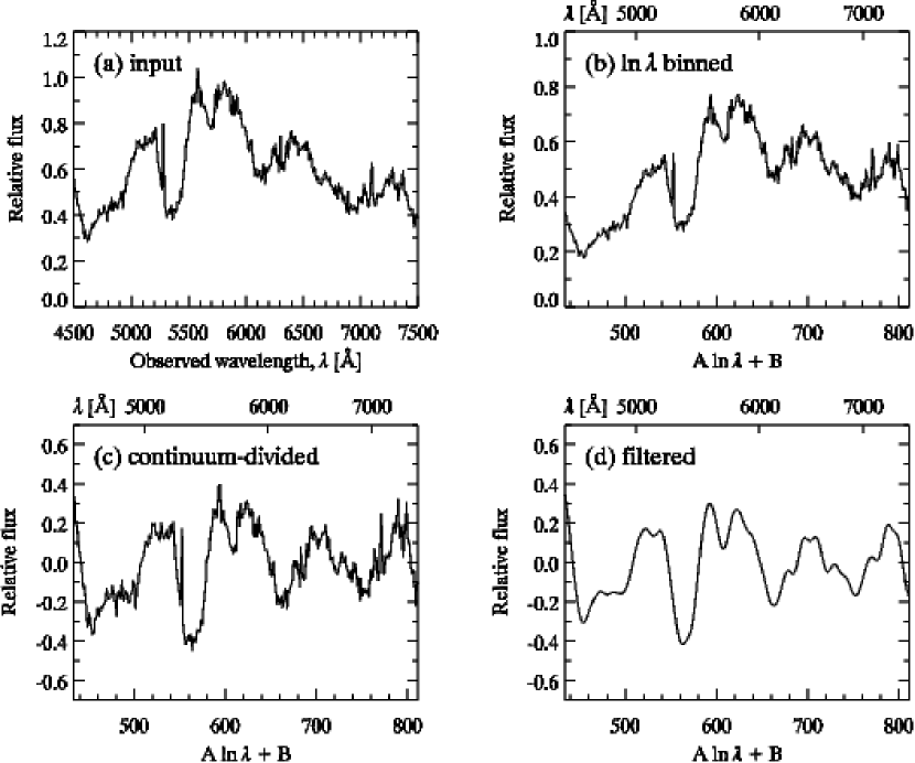
Figure 1.— Pre-processing the spectrum for SNID. (a) Spectrum of the SN Ia SN 2003lj at $z=0.417$ (Matheson et al., 2005). (b) The result of mapping the spectrum to $\ln\lambda$ coordinates, with $(\lambda_{0},\lambda_{1},N)=(2500$ Å$,10000$ Å$,1024)$. (c) A 13-point spline has been divided out and the result normalized to zero mean flux. (d) A bandpass filter with $(k_{1},k_{2},k_{3},k_{4})=(1,4,25,102)$ has been applied to the spectrum.

The next step in preparing the spectra for correlation analysis is continuum removal (Tonry & Davis, 1979). For galaxy spectra, the continuum is well defined and is easily removed using a least-squares polynomial fit. In supernova spectra, however, the apparent continuum is ill-defined due to the domination of bound-bound transitions in the total opacity (Pinto & Eastman, 2000). Dividing out a 13-point cubic spline fit to the spectrum (over the entire 2500–10000 Å wavelength interval) is akin to removing a pseudo continuum from the supernova spectrum. We then subtract 1 from the resulting spectrum and apply a normalization constant for the mean flux to equal zero (Fig. 1c). This effectively discards any spectral color information (including reddening uncertainties and flux mis-calibrations), and the correlation only relies on the relative shape and strength of spectral features in the input and template spectra. We note that continuum division is also used by Jeffery et al. (2006) for measuring the goodness-of-fit between supernova spectra. We see below (§ 5) that the loss of color information has surprisingly little impact on the redshift and age determination. Continuum removal also minimizes discontinuities at each end of the spectrum, which would cause artificial peaks in the correlation function. Further discontinuities are removed by apodizing the spectra with a cosine bell ($\sim 5\%$ at either end).

The final step is the application of a bandpass filter. While it is actually applied at a later stage, directly to the correlation function, we show its effect on the input spectrum in Fig. 1d. The goal is to remove low-frequency residuals left over from the pseudo-continuum removal and high-frequency noise components. Formally, the Fourier transform of the normalized correlation function, $C(k)$ (eq. 6), is multiplied by a real bandpass function (so that no phase shifts are introduced) $B(k)$, such that

$$B(k)=\left\{\begin{array}[]{ll}0&\textrm{for $k\leq k_{1}$ or $k\geq k_{4}$}\\ \text@frac{1}{2}\left[1-\cos\left(\frac{k-k_{1}}{k_{2}-k_{1}}\right)\right]&\textrm{for $k_{1}<k<k_{2}$}\\ 1&\textrm{for $k_{2}\leq k\leq k_{3}$}\\ \text@frac{1}{2}\left[1-\cos\left(\frac{k-k_{3}}{k_{4}-k_{3}}\right)\right]&\textrm{for $k_{3}<k<k_{4}$}\\ \end{array}\right.$$ (15)

The exact choices for the wavenumbers $(k_{1},k_{2},k_{3},k_{4})$ depend on the size of each $k$ bin and on the spectral energy distribution of a supernova spectrum. Supernova spectral lines have typical widths of $\sim$100–150 Å, due to the large expansion velocities of the ejecta ($\sim 10000$  km s^-1). The mean size of a logarithmic wavelength bin with $(\lambda_{0},\lambda_{1},N)=(2500$ Å$,10000$ Å$,1024)$ is $\sim 7.2$ Å, so a typical SN line will have a width $w_{\rm line}\sim$ 14–21 logarithmic wavelength bins. In Fourier space, most of the information will be at wavenumbers $k=N/(2\pi\times w_{\rm line})\approx$ 8–12. Since SN spectra consist of overlapping spectral lines (Baron et al., 1996), a typical SN feature may have a lower width ($\lesssim 50$ Å). This translates to $k\sim 25$, so most information is at wavenumbers less than 25 and almost everything above wavenumber $k\sim 50$ is noise. Also, low wavenumbers ($k\lesssim 5$) contain information about the low-frequency residuals from continuum removal. In Fig. 2 we show the amplitude of the Fourier transform of typical unfiltered correlation functions as a function of wavenumber. As expected, most of the correlation power is at wave numbers $k\sim$ 10–20, and virtually no information is contained in wavenumbers $k>50$.

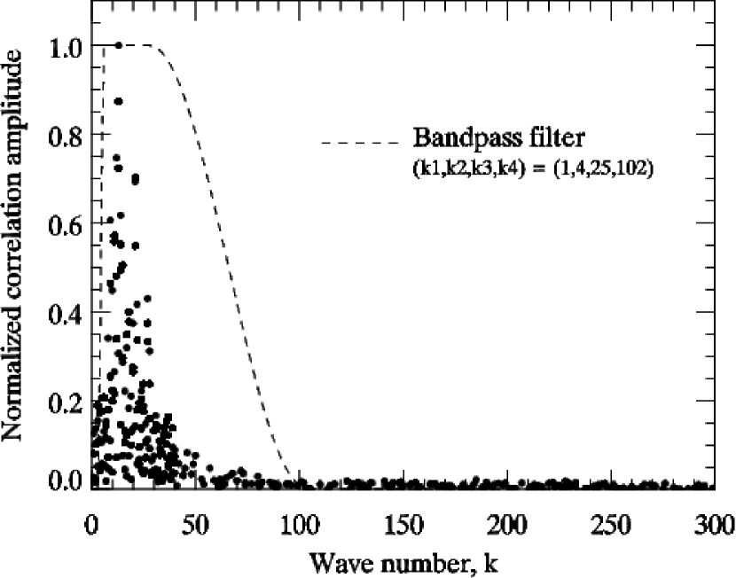
Figure 2.— Normalized amplitude of the Fourier transform of typical unfiltered cross-correlation functions vs wavenumber, $k$. Note how most of the power is concentrated at low wavenumbers ($k\lesssim 50$), justifying our choice for the bandpass filter (dashed line). In this example the maximum correlation amplitude is at $k=13$, corresponding to a wavelength scale of $\sim 90$ Å.

3. Redshift Estimate

In this section we introduce the correlation height-noise ratio $r$ (§ 3.1) and the spectrum overlap (${\rm lap}$) parameter (§ 3.2), the product of which (the $r{\rm lap}$ quality parameter) conveys quantitative information about the reliability of a cross-correlation redshift output by SNID. We then briefly describe the redshift estimation (§ 3.3) and associated error (§ 3.4).

3.1. The $r$-value

Tonry & Davis (1979) introduce the correlation height-noise ratio, $r$, to quantify the significance of a peak in the normalized correlation function, $c(n)$. It is defined as the ratio of the height, $h$, of the peak to the rms of the antisymmetric component of $c(n)$, $\sigma_{a}$, about the correlation redshift (Fig. 3):

$$r=\frac{h}{\sqrt{2}\sigma_{a}}.$$ (16)

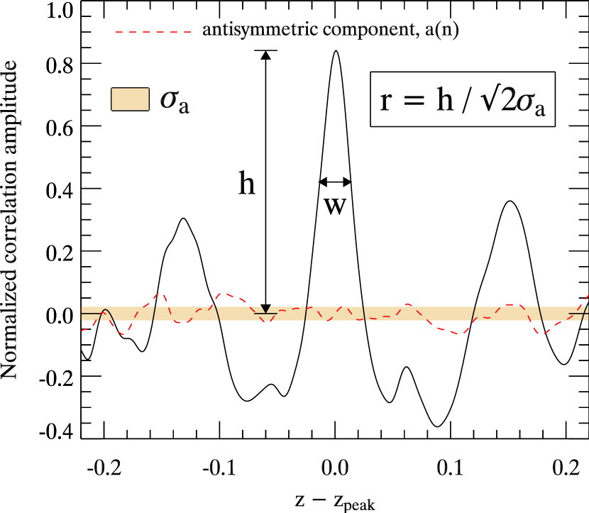
Figure 3.— Correlation height-noise ratio, $r$, is defined as the ratio of the height, $h$, of the highest peak in the normalized correlation function (solid line) to the rms of its antisymmetric component, $a(n)$ (dashed line), about the redshift corresponding to that peak ($z_{\rm peak}$). The width of the peak, $w$, is used to compute the redshift error (see text for details). [See the electronic version of the Journal for a color version of this figure.]

In order to compute $\sigma_{a}$, Tonry & Davis (1979) assume that $c(n)$ is the sum of an auto-correlation of a template spectrum $t(n)$ with a shifted template spectrum $t(n-\delta)$ and of a random function $a(n)$ that can distort the correlation peak:

$$c(n)\equiv t(n)\star t(n-\delta)+a(n).$$ (17)

The first term on the right-hand side of eq. 17 is supposed to give a correlation peak of height $h=1$ at the exact redshift (corresponding to a shift $\delta$ in logarithmic wavelength units), while the second part can distort the peak. Since $t\star t(n-\delta)$ is symmetric about $n=\delta$, the antisymmetric part of $c(n)$ about $n=\delta$ equals the antisymmetric part of $a(n)$ about $n=\delta$. We further assume that the symmetric part of $a(n)$ has roughly the same amplitude as its antisymmetric part and that the symmetric and antisymmetric parts of $a(n)$ are uncorrelated. In that case, the rms of $a(n)$ is $\sqrt{2}$ times the rms of its antisymmetric component.

A perfect correlation will have a peak with $h=1$ at the exact redshift, and $c(n)$ will be symmetric about $n=\delta$, thus $\sigma_{a}=0$ and so $r\longrightarrow\infty$ (Fig. 4, left panel). Conversely, $r$ will be small ($r\lesssim 5$) for a spurious correlation peak (Fig. 4, right panel), and large ($r\gtrsim 10$) for a significant peak, since $h$ will be close to 1 and $\sigma_{a}$ will be small (Fig. 4, middle panel).

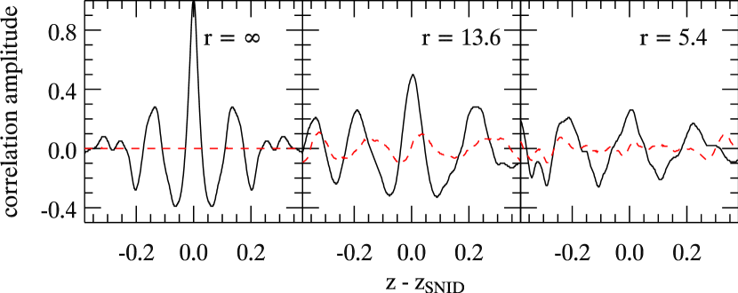
Figure 4.— Examples of perfect (left), good (middle), and poor (right) normalized correlation functions (solid line). The antisymmetric component of the correlation function about the SNID redshift ($z_{\rm{\rm SNID}}$) is also shown (dashed line). [See the electronic version of the Journal for a color version of this figure.]

3.2. Spectrum Overlap

In SNID, the correlation height-noise ratio $r$ alone does not provide the estimator by which a correlation peak is deemed reliable. It is further weighted by the overlap in $\ln\lambda$ space between the input spectrum and each of the template spectra used in the correlation. In practice, the template spectra are trimmed to match the wavelength range of the input spectrum at the redshift corresponding to the correlation peak. For an input spectrum with rest-frame wavelength range $[\lambda_{0},\lambda_{1}]$, the overlap in $\ln\lambda$ space, ${\rm lap}$, with each template spectrum is in the range

$$0\leq{\rm lap}\leq\ln{\left(\frac{\lambda_{1}}{\lambda_{0}}\right)}.$$ (18)

Thus for an input and template spectra both overlapping the rest-frame wavelength interval 3500–6000 Å, ${\rm lap}=\ln(6000/3500)\approx 0.54$.

The spectrum overlap parameter conveys important absolute information about the quality of the correlation, complementary to the correlation height-noise ratio $r$. Supposing a typical SN Ia spectral feature has an FWHM of $\Delta\lambda\approx 200$ Å at $\lambda\approx 5000$ Å, any correlation with ${\rm lap}\lesssim\ln{(5400/5000)}\approx 0.08$ will be meaningless: any feature will match any other at practically any redshift. Only when a correlation has an associated ${\rm lap}$ that is several times $\ln{(\Delta\lambda/\lambda)}$ can one rely on the redshift output by SNID.

In what follows, we usually discard correlation redshifts that have an associated ${\rm lap}<{\rm lap}_{\rm min}=0.4$ and a quality parameter $r{\rm lap}=r\times{\rm lap}<r{\rm lap}_{\rm min}=5$. In Fig. 5 we show contour plots for both the ${\rm lap}$ and $r{\rm lap}$ parameters, central to the use of SNID.

Figure 5.— Top: Contours of equal ${\rm lap}=\ln(\lambda_{1}/\lambda_{0})$ for different rest-frame wavelength ranges $[\lambda_{0},\lambda_{1}]$ of overlap between input and template spectra. We usually discard correlations with ${\rm lap}<0.4$. Bottom: Contours of equal $r{\rm lap}=r\times{\rm lap}$ for a broad range of values for the correlation height-noise ratio ($r$) and spectrum overlap parameter (${\rm lap}$). We usually discard correlations with $r{\rm lap}<5$ (and ${\rm lap}<0.4$).

3.3. Initial and Revised Redshift Estimates

For each template spectrum $t_{i}(n)$, we compute the correlation function $c_{i}(n)=s(n)\star t_{i}(n)$. In general, $c_{i}(n)$ has many peaks in redshift space (Fig. 3,4). The true redshift is most likely the one corresponding to the highest peak in $c_{i}(n)$, although in poor signal-to-noise ratio cases some peaks can distort or surpass the true redshift peak (Fig. 4, right panel). In practice, SNID selects the 10 highest peaks (labeled with index $j$) in $c_{i}(n)$ one by one and performs a fit with a smooth function to determine the peak height and position, $h_{ij}$ and $\delta_{ij}$, respectively. The corresponding redshift is $z_{ij}=\exp(\delta_{ij}d\lambda_{\rm ln})-1$. The wavelength regions of $s(n)$ and $t_{i}(n)$ that do not overlap at $z_{ij}$ are trimmed, and, if the resulting spectrum overlap ${\rm lap}\geq{\rm lap}_{\rm min}$, a new “trimmed” correlation function, $c_{ij}(n)$, is computed, and the corresponding correlation height-noise ratio ($r_{ij}$), spectrum overlap (${\rm lap}_{ij}$), and redshift ($z_{ij}$) are stored.

Once all templates have been cross-correlated with the input spectrum, SNID computes an initial redshift, $z_{\rm init}$, based on an $r{\rm lap}$-weighted median of all $z_{ij}$. Each redshift $z_{ij}$ is replicated $W_{ij}$ times according to the following weighting scheme:

$$W_{ij}=\left\{\begin{array}[]{ll}5&\quad\textrm{for $\quad r{\rm lap}_{ij}>6$}\\ 3&\quad\textrm{for $\quad r{\rm lap}_{ij}>5$}\\ 1&\quad\textrm{for $\quad r{\rm lap}_{ij}>4$}\\ 0&\quad\textrm{for $\quad r{\rm lap}_{ij}\leq 4$,}\\ \end{array}\right.$$ (19)

If all $r{\rm lap}_{ij}\leq 4$, $z_{\rm init}$ is set to 0.

SNID then computes a revised redshift based on the initial estimate, $z_{\rm init}$. The input and template spectra (again labeled $i$) are trimmed such that their wavelength coverage coincides at $z_{\rm init}$. If the resulting spectrum overlap ${\rm lap}_{i}\geq{\rm lap}_{\rm min}$, a second trimmed correlation function is computed and the correlation height-noise ratio ($r_{i}$), spectrum overlap (${\rm lap}_{i}$), and redshift ($z_{i}$) corresponding to the highest correlation peak are stored. The width $w_{i}$ of the correlation peak is also saved and is used to compute the redshift error (see next section). The revised redshift, $z_{{\rm SNID}}$, is computed as the non-$r{\rm lap}$-weighted median of all redshifts $z_{i}$ that satisfy $r{\rm lap}_{i}\geq r{\rm lap}_{\rm min}$ with ${\rm lap}_{i}\geq{\rm lap}_{\rm min}$, with the additional requirement that the individual redshifts $z_{i}$ do not differ significantly from the initial redshift estimate: $|z_{i}-z_{\rm init}|<z_{\rm filt}$, where $z_{\rm filt}=0.02$, typically.

3.4. Redshift Error

One of the advantages of using the cross-correlation technique for redshift determination is the ability to estimate the redshift error, $\epsilon_{z}$. Tonry & Davis (1979) derive a formal expression for $\epsilon_{z}$ based on the idea that spurious peaks (positive and negative) in the antisymmetric component, $a(n)$, of the correlation function, $c(n)$, can distort the true correlation peak. Obviously, $\epsilon_{z}$ is proportional to the number of peaks in $a(n)$, and hence to the mean distance between peaks. Assuming $c(n)$ and $a(n)$ have similar power spectra, the mean distance between a peak in $c(n)$ and the nearest peak in $a(n)$ can be estimated as $N/8B$ (Tonry & Davis 1979, their eq. 22), where $N$ is the total number of bins and $B$ is the highest wavenumber at the half-maximum point of the Fourier transform of $c(n)$ ($B\approx 25$ here; see Fig. 2). One can then show that (Tonry & Davis 1979, their eq. 24)

$$\epsilon_{z}=k_{z}\times\frac{1}{1+r},$$ (20)

where $k_{z}=N/8B$ ($\approx 5$ here) and $r$ is the correlation height-noise ratio defined in eq. 16. With the additional assumption of sinusoidal noise in $c(n)$, Kurtz & Mink (1998) find $k_{z}=3w/8$, where $w$ is the width of the correlation peak.

In practice, $k_{z}$ is calibrated using additional redshift measurements, either through a different technique (e.g., 21 cm measurements for galaxy redshifts in Tonry & Davis 1979) or using the same cross-correlation technique on two spectra of the same object (Kurtz & Mink, 1998). For supernova spectra, additional redshift information potentially comes from narrow emission and absorption lines in the host galaxy, while duplicate spectra of the same supernova (at the same age) are not common (Table Determining the Type, Redshift, and Age of a Supernova Spectrum). We find that including the spectrum overlap parameter (${\rm lap}$) yields a more robust estimator of the redshift error (see also § 5.2):

$$\epsilon_{z}=k_{z}\times\frac{1}{1+r{\rm lap}},$$ (21)

with $k_{z}\approx$ 2–4$w$.

4. The SNID Database

4.1. Nomenclature and Age Distribution

The current SNID spectral database comprises 879 spectra of 65 SNe Ia, 322 spectra of 19 SNe Ib/c, and 353 spectra of 10 SNe II (Table Determining the Type, Redshift, and Age of a Supernova Spectrum). The spectra are drawn from public archives (SUSPECT and the CfA Supernova Archive) and from the CfA Supernova Program (Matheson et al., 2007). The spectra are chosen to have high signal-to-noise ratio (typically $\gtrsim 10$ per Å) and to span a sufficiently large optical rest frame wavelength range ($\lambda_{\rm min}\leq 4000$ Å; $\lambda_{\rm max}\geq 6500$ Å) to include all the identifying features of SN spectra. We remove telluric features in all the spectra, either using the well-exposed continua of spectrophotometric standard stars for the CfA data (Wade & Horne, 1988; Matheson et al., 2000), or using a simple linear interpolation over the strong A- and B-bands. We show the full suite of spectra for the local SN Ia spectral template SN 1992A (Kirshner et al., 1993), which also includes some UV data from the Hubble Space Telescope at some epochs, shifted to zero redshift in Fig. 6.

While we have included all the supernovae available to us for which there are a large number of epochs of spectroscopy, there are still many more ($>1000$) supernovae for which there are only one to two epochs of spectroscopy that we have yet to include in the database. We also include spectra of galaxies, active galactic nuclei, stars (including variable stars, such as luminous blue variables), and novae. This can be particularly useful when trying to weed out contaminants from large surveys of high-redshift supernovae (cf. Matheson et al. 2005).

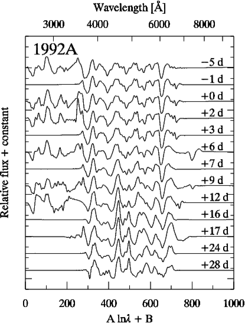
Figure 6.— Example of an SNID template, here the SN Ia SN 1992A (Kirshner et al., 1993). We also indicate the age of each spectrum (in days from $B$-band maximum). Discontinuities in flux around $\sim 3500$ Å are due to a calibration mismatch between the UV and optical components of the spectrum.

We show the age distribution of SNID supernova templates for the main supernova types (Ia, Ib, Ic, II) in Fig. 7. For each type, we show the age distribution of “normal” representatives of that type, as well as spectra that show deviations from the latter (in the “other” category). We note that this division is somewhat qualitative and relies on the identification by eye of certain characteristic spectroscopic features in the spectra (Filippenko, 1997). We are currently working on a statistical scheme to separate our template spectra in these various categories (see also Fig. 8). The nomenclature for the different supernova types and their associated subtypes is given in Table 2. From Fig. 7, it is clear that the age distribution of the SNID templates is not uniform, and even bi-modal for SNe Ia. This potentially introduces age “attractors” that could in principle bias the age and redshift determination (although see § 5). The fact that there are more SN Ia templates than SNe Ib, Ic, and II combined also leads to a type “attractor,” with the risk for low-S/N spectra to be preferentially classified as SN Ia, regardless of their type (see § 6).

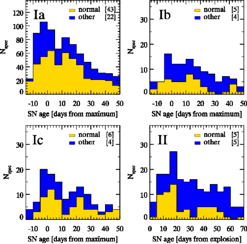
Figure 7.— Age distributions of SNID templates for supernovae of different types. The number of supernovae corresponding to a given type is indicated in square brackets. Note the larger ordinate range for SNe Ia. For SNe II, the age is given in days from the estimated date of explosion as opposed to days from maximum in a specific band. The transitional SNe IIb are included in both Type Ib and Type II histograms. [See the electronic version of the Journal for a color version of this figure.]

Table 2Supernova types and subtypes

Type	Ia	Ib	Ic	II
“normal”	Ia-norm	Ib-norm	Ic-norm	II-norm (IIP)
	Ia-pec	Ib-pec	Ic-pec	II-pec
“other”	Ia-91T	IIb	Ic-broad	IIL
	Ia-91bg			IIn
				IIb

Note. — “norm” and “pec” refer to “normal” and “peculiar” subtypes of the corresponding type; see Table Determining the Type, Redshift, and Age of a Supernova Spectrum for specific examples. “Ic-broad” is used to identify broad-lined SNe Ic (“hypernovae”), some of which are associated with Gamma-Ray Bursts. The transitional Type IIb supernovae are included in both Type Ib and Type II categories.

The execution time of SNID scales linearly with the number of templates and is remarkably low compared with $\chi^{2}$-based methods (see § 7)— although see Rybicki & Press (1995) for fast statistical methods that can compete with the cross-correlation technique. It is trivial to include large spectroscopic data sets— such as those from the CfA Supernova Group (for example, 431 spectra of 32 SNe Ia, included in the present SNID database, will soon be published by Matheson et al. 2007).

4.2. Intrinsic Spectral Variance

In Fig. 8 we show the standard and maximum deviation from the mean spectrum of all “Ia-norm” templates at $-10$, +0, +10, and +20 days from maximum light. One clearly sees the rapid variation of SN spectra around maximum light, but also the change in intrinsic scatter with age. For instance, the intrinsic spread in the strength and position of the defining Si ii $\lambda$6355 feature (which causes the deep blueshifted absorption around $\sim 6100$ Å) decreases between $-10$ to $+10$ days from maximum light. At +20 days, the scatter is large in that wavelength region due to increasing contribution from other ions (mainly Fe ii).

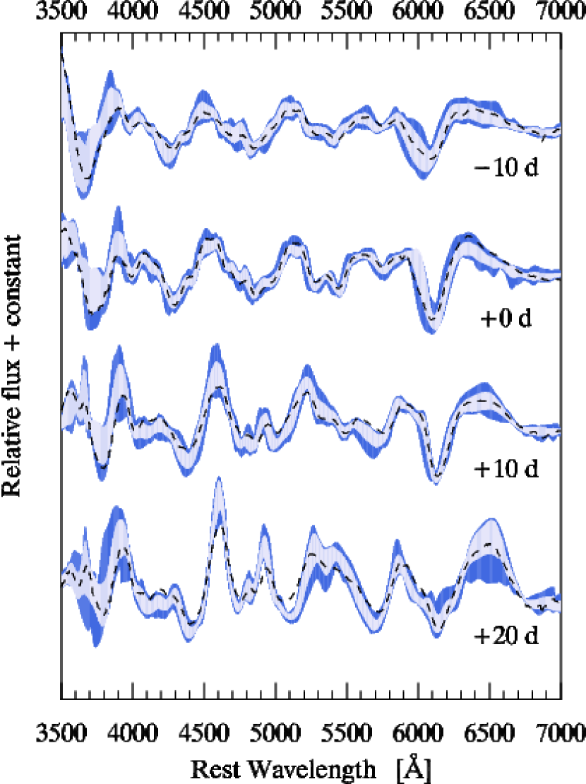
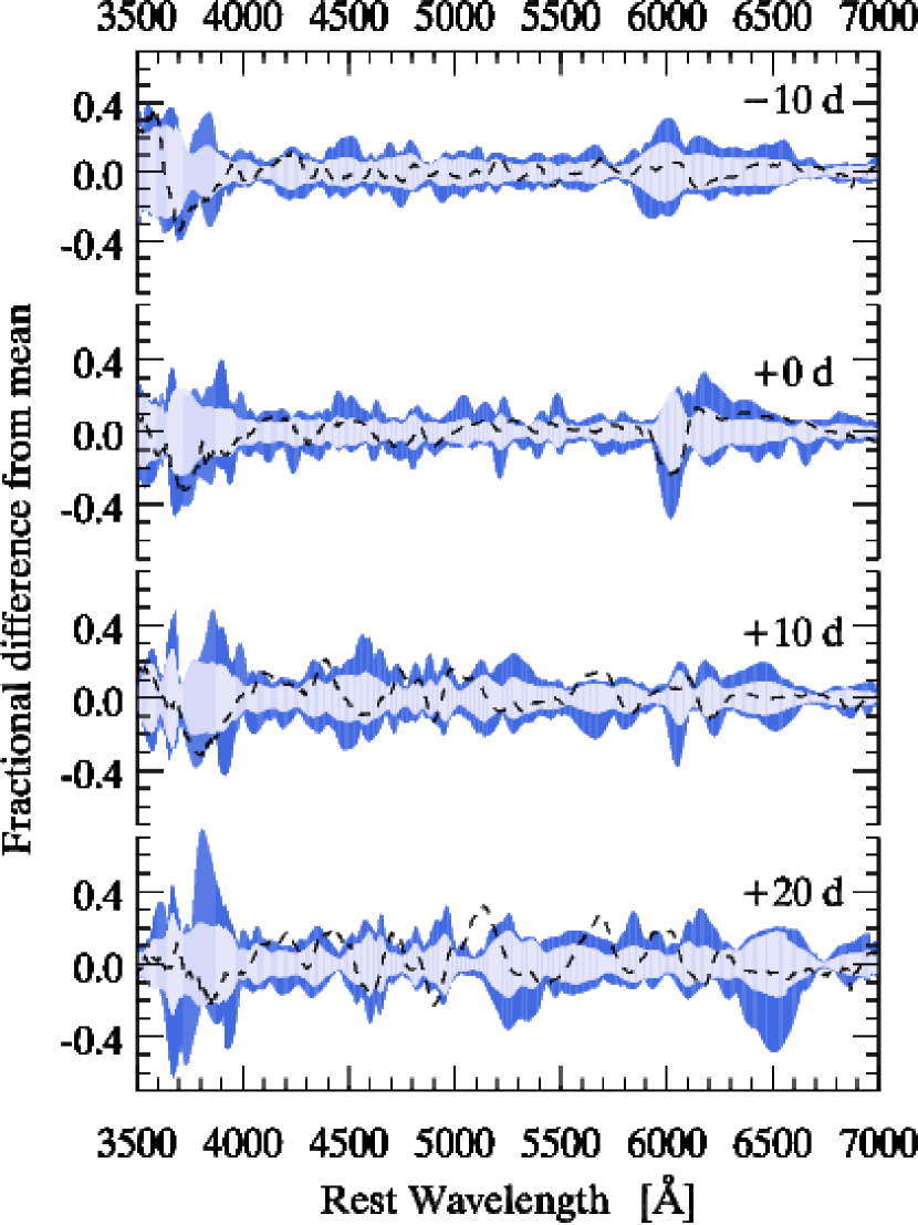
Figure 8.— Left: Standard (light gray) and maximum (dark gray) deviation from the mean spectrum for all Ia-norm templates, at four different ages. We overplot the corresponding Nugent template at each age (dashed line). All spectra have been pre-processed in the same way as any SNID template (§ 2.3). Right: Fractional difference from the mean Ia-norm spectrum. We also show the ratio of the mean spectrum to the corresponding Nugent template (dashed line). [See the electronic version of the Journal for a color version of this figure.]

The residual variation about the mean spectrum (Fig. 8, right panel) shows that normal SNe Ia are typically within 10%–20% from the mean spectrum, although deviations greater than 40% are seen at certain wavelength intervals (again depending on the age). The fact that all Ia-norm template spectra are within two standard deviations from a mean spectrum suggests a possible statistical classification scheme to differentiate normal SNe Ia from the other Ia subtypes. With more data, it is in principle possible to do this more reliably for SNe Ia, as well as other supernova types.

The intrinsic variation of the Ia-norm templates points to the inadequacy of describing a given SN subtype with a single representative template, unless the latter includes this variance explicitly. Past attempts to create grids of such template spectra, such as those presented by Nugent et al. (2002), do not account for the variability within a given SN type at a given age. We show the corresponding Nugent template (ver. 1.2) at each age in Fig. 8 (dashed line). While most of the Nugent template is included within the standard deviation from the mean spectrum in our database, there are also significant deviations. We do note, however, that the comparison is somewhat misleading since Nugent et al. (2002) had less data available to them for the elaboration of these templates. Nevertheless, we have tested their use in the SNID spectral database, but have found them to lead to systematic errors in both the redshift and age determination.

5. Accuracy of Redshift and Age Determination

We use a simple simulation to test the accuracy of SNID in determining the redshift and age of a supernova spectrum. Here we focus on normal SNe Ia since they are the most represented in our spectral database, although the conclusions of this section are qualitatively valid for all other supernova types. Even though normal SNe Ia form a homogeneous class, the spectra reveal intrinsic variations at any given age that affect directly the redshift and age determination. The redshift precision depends primarily on the typical width of a spectral feature (decreasing from broad-lined SNe Ic to SNe IIn), which affects the width of the correlation peak (see Fig. 3). The redshift accuracy depends primarily on the intrinsic variation of line positions at a given age. The age determination strongly correlates with the redshift determination (§ 5.4), and depends on how quickly the SN spectra evolve at a given age.

5.1. Presentation of the Simulation

In this simulation, each Ia-norm spectrum in the SNID database (cf. Table Determining the Type, Redshift, and Age of a Supernova Spectrum) is correlated with all other Ia-norm spectra, except for those corresponding to the input supernova (to ensure unbiased results). We require all spectra used in the simulation to include the rest-frame wavelength interval 3700–6500 Åand to have an age (in days from $B$-band maximum, hereafter $t_{B}$) $-10\leq t_{B}\leq+20$.

We show the simulation parameters in Table 3. The input spectrum is first redshifted to $z$ by simply multiplying the wavelength axis by $(1+z)$. We then “contaminate” the input supernova spectrum with galaxy light (up to 50% of the total flux), using the elliptical and Sc galaxy templates of Kinney et al. (1996), and add noise (both random Poisson noise and sky background) to reproduce the range of typical signal-to-noise ratio of SN spectra at the simulation redshifts, when observed with 6.5–10 m-class telescopes (e.g., VLT, Keck, Gemini, Magellan) used in cosmological SN Ia surveys. Note that we do not scale the input spectral flux to match a given simulation redshift, as SNID normalizes the input and template spectra in a similar fashion (Fig. 1).

Table 3Simulation parameters

Parameter	Range
Redshift, $z$	$0.1\leq z\leq 0.7$
Galaxy contamination fraction, $f_{\rm gal}$	$0\leq f_{\rm gal}\leq 0.50$
Signal-to-noise ratio, S/N (per 2 Å)	$1\leq{\rm S/N}\leq 15$
Age (days from $B$-band maximum), $t_{B}$	$-10\leq t_{B}\leq+20$
Minimum rest frame wavelength coverage, $\lambda_{\rm rest}$ (Å)	$3700\leq\lambda_{\rm test}\leq 6500$
Observed wavelength range, $\lambda_{\rm obs}$ (Å)	$4000\leq\lambda_{\rm obs}\leq 9000$

We restrict the observed wavelength range over which SNID computes the correlation to $4000\leq\lambda_{\rm obs}[$Å$]\leq 9000$, to mimic the coverage of the FORS1 optical spectrograph mounted on the VLT. We have not studied the impact of a change in this wavelength range on the redshift or age determination. Furthermore, we force SNID to only consider correlation redshifts in the interval $[0,1]$. For each correlation, we record the template name, type, subtype, and age; the correlation redshift and its associated correlation height-noise ratio ($r$) and spectrum overlap parameter (${\rm lap}$); and the width $w$ of the correlation peak (to estimate the redshift error).

To study the effects of constraints on redshift and age, we run SNID three times on the input spectrum: once with no constraints; a second time with a flat constraint on redshift ($\pm 0.01$), and a third time with a flat constraint on age ($\pm 3$ days). We note that the distribution of redshift residuals is remarkably Gaussian (§ 5.2), and we are currently implementing Gaussian priors in SNID. A total of 4 billion correlations were computed with SNID for this simulation, in just under 70 CPU hr.

5.2. Redshift Residuals and Redshift Error

We show the distribution of redshift residuals, $\Delta z$, versus the $r{\rm lap}$ quality parameter in the top-right panel of Fig. 9, for input parameters $0.3\leq z\leq 0.5$, $-5\leq t_{B}\leq+15$, and $2\leq$ S/N (per 2 Å)$\leq 10$. The residuals are shown as a two-dimensional (2D) histogram, with a linear gray-scale scheme reflecting the number of points in a given $(\Delta z,r{\rm lap})$ bin. We only show correlations for which the overlap between input and template spectra ${\rm lap}\geq 0.4$. For good correlations ($r{\rm lap}\gtrsim 5$), the distribution of redshift residuals is a Gaussian centered at $\Delta z=0$. In the bottom right panel, we show the standard deviation of redshift residuals, $\sigma_{z}$, in $r{\rm lap}$ bins of size unity. For $r{\rm lap}\gtrsim 5$, we have a typical error in redshift of order $\sigma_{z}\lesssim 0.01$.

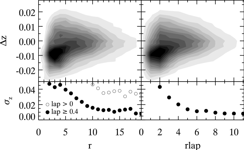
Figure 9.— Top: 2D histograms of redshift residuals vs. the correlation height-noise ratio $r$ (left panel) and the $r{\rm lap}$ quality parameter (with ${\rm lap}\geq 0.4$; right panel), with the following parameters: $0.3\leq z\leq 0.5$, $-5\leq t_{B}\leq+15$, $2\leq$ S/N (per 2 Å)$\leq 10$. The linear gray scale reflects the number of points in a given 2D bin (the more points the darker). Bottom: Standard deviation, $\sigma_{z}$, of redshift residuals in $r,r{\rm lap}$ bins of size unity. For the $\sigma_{z}(r)$ curve (filled circles, bottom left), we show the effect of additionally requiring that ${\rm lap}\geq 0.4$ (open circles).

For poor correlations ($r{\rm lap}\lesssim 3$) there is a concentration of points around $\Delta z\approx-0.01$. This is an artifact of the pseudo-continuum removal, which enhances the contrast between emission peaks and absorption troughs in the input and template spectra and biases poor correlations to later ages. In this simulation, many input spectra at maximum are attracted to $\sim+10$ days, where the position of SN spectral features has shifted redward in wavelength due to the expansion of the supernova envelope (Fig. 10). The template needs to be shifted less in $\ln\lambda$ space to match the redshift of the input spectrum, which leads to an under-estimation of the redshift by $\sim 0.01$. This corresponds to a combination of the typical velocity shift in SN Ia absorption features from maximum to $\sim 10$ days past maximum, and the spread of these velocities at a given age ($\sim 3000$ km s^-1; see Benetti et al. 2005; Blondin et al. 2006a). We note that this artifact has no impact on correlations with $r{\rm lap}>3$.

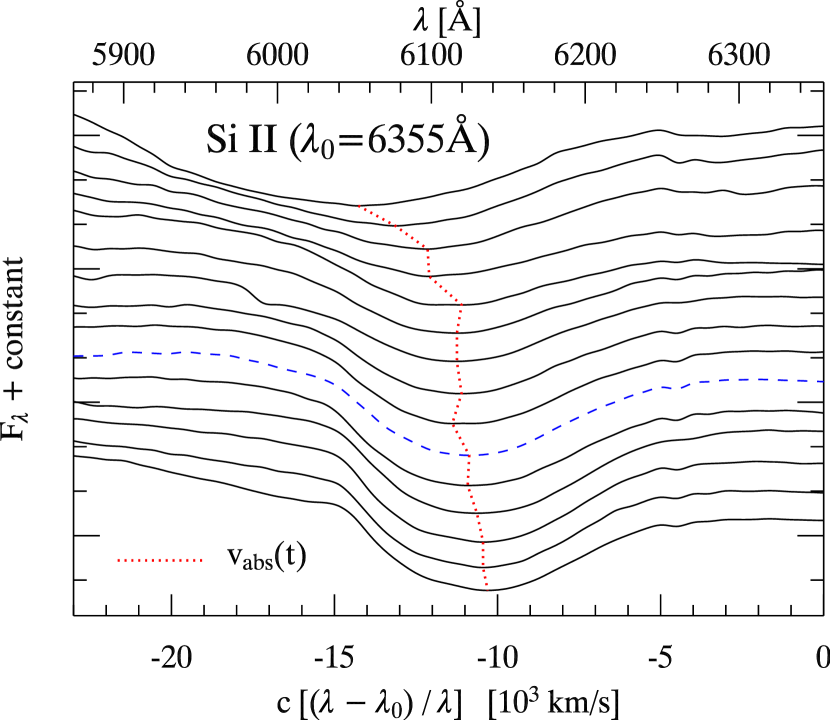
Figure 10.— Evolution of the blueshifted Si ii $\lambda$6355 absorption profile in the SN Ia SN 1994D (Höflich, 1995; Patat et al., 1996) between $-11$ and +7 days from $B$-band maximum. The dotted line shows the velocity location of the locus of maximum absorption, $v_{\rm abs}$. We highlight the Si ii profile at maximum light (dashed line). Over the course of 18 days, the locus of maximum absorption shifts redward in wavelength by $\sim 80$ Å, corresponding to $\sim 4000$  km s^-1 in velocity. Note the more rapid evolution of $v_{\rm abs}$ before maximum light. [See the electronic version of the Journal for a color version of this figure.]

In the left panels of Fig. 9, we show the same distribution of $\Delta z$, this time only as a function of the correlation height-noise ratio, $r$ (note the change in the abscissa range). To first order, the 2D histogram of redshift residuals looks remarkably similar to that as a function of $r{\rm lap}$ (Fig. 9, right panels), with again a concentration of points around $\Delta z\approx-0.01$ for low values of $r$. However, the variation of $\sigma_{z}$ with $r$ (bottom left panel, filled circles) gives a different picture: the lack of constraint on ${\rm lap}$ causes in some cases a mis-estimate of the redshift, at all $r$, thereby greatly biasing $\sigma_{z}$ to higher values ($\sigma_{z}>0.03$, for all $r$). Requiring that ${\rm lap}\geq 0.4$ leads to a significant improvement (open circles), with $\sigma_{z}\lesssim 0.01$ for $r\gtrsim 10$. It is therefore imperative to consider the overlap between the input and template spectra to yield accurate supernova redshifts with the cross-correlation technique.

The formal redshift error, $\epsilon_{z}$, is proportional to $w/(1+r{\rm lap})$ (eq. 21), $w$ being the width of the correlation peak (Fig. 3). We illustrate the determination of the constant of proportionality, $k_{z}$, in Fig. 11, where we show the same 2D histograms of redshift residuals $\Delta z$, this time as a function of $(1+r)/w$ (left panels) and $(1+r{\rm lap})/w$ (right panels). A best fit to the $\sigma_{z}$ curves in the bottom panels yields a value for $k_{z}$: 5.3 for $(1+r)/w$, and 3.1 for $(1+r{\rm lap})/w$. Only correlations with ${\rm lap}\geq 0.4$ are shown. As in Fig. 9, the product of the $r$-value and the overlap yields a more robust error estimator than the $r$-value alone. In what follows we study variations of redshift and age determinations using SNID only as a function of the $r{\rm lap}$ quality parameter, with ${\rm lap}\geq 0.4$.

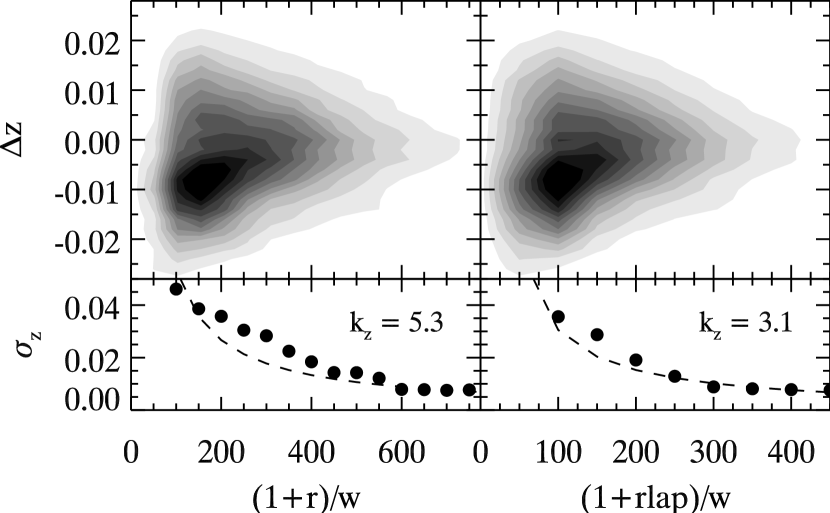
Figure 11.— Same as Fig. 9, except the abscissae now correspond to $(1+r,r{\rm lap})/w$, where $w$ is the width of the correlation peak. A fit to the binned $\sigma_{z}$ distributions (bottom) yields the value for $k$ used in estimating the error (eq. 21). In both panels, only correlations with ${\rm lap}\geq 0.4$ are shown.

In principle, $k_{z}$ needs to be evaluated for every template spectrum in the database, through either internal or external comparisons (as done for galaxy spectral templates in Tonry & Davis 1979; Kurtz & Mink 1998). While this is impractical for supernova spectra— there are few duplicate spectra of the same supernova at a given age (Table Determining the Type, Redshift, and Age of a Supernova Spectrum), we have computed $k_{z}$ using subsets of templates used in our simulation, as well as for other supernova types, and have found that $k_{z}$ is typically in the range $2\lesssim k_{z}\lesssim 4$, with $k_{z}\approx 3$ being the median value.

The above holds for a single spectral template; to use SNID to its full capacity, we need to combine redshifts for all templates for which the $r{\rm lap}$ quality parameter is greater than a certain cutoff (generally, $r{\rm lap}\geq r{\rm lap}_{\rm min}=5$). In § 3.3, we favored the non-$r{\rm lap}$-weighted median of all correlation redshifts with $r{\rm lap}\geq r{\rm lap}_{\rm min}$ as being “the” SNID redshift, but did not justify this. In Fig. 12 (top panels), we show distributions of SNID redshift residuals, when the SNID redshift is taken to be the redshift corresponding to the highest $r{\rm lap}\geq 5$ value (“best;” left panel); the median (middle panel) or $r{\rm lap}$-weighted mean (right panel) of all redshifts with $r{\rm lap}\geq 5$. Both the median and mean distributions are consistent with a Gaussian distribution, with the median redshift providing a slightly better match. This is expected since the use of the median redshift guards us from systematic errors produced by spurious or ill-defined correlation peaks for some templates. The distribution of “best” redshift residuals is broader and non-uniform. We therefore consider the median redshift to provide the best estimate.

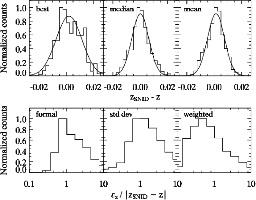
Figure 12.— Top: Normalized distributions of redshift residuals, when the SNID redshift is assumed to be the redshift of the best-match template (left), the median redshift (middle), and the $r{\rm lap}$-weighted mean redshift (right). The distribution of median redshifts is the most consistent with a normal distribution. Bottom: Normalized distributions of the ratio of the absolute redshift residual (corresponding to the different redshift estimators in the top panel) to the redshift error, $\epsilon_{z}$, estimated in different ways (see text for details).

In the bottom panels of Fig. 12 we show the normalized distributions of the ratio of the absolute redshift residual (corresponding to the different redshift estimators in the top panel) to the redshift error, $\epsilon_{z}$, estimated in different ways. A ratio equal to or above unity indicates that the actual redshift is consistent with the SNID redshift within the estimated error, while a ratio below unity indicates that the error is under-estimated. For a good error estimator, we expect those distributions to peak at a ratio near unity, with a long tail to higher ratios and a sharp drop below unity. Such is the case for the formal redshift error (eq. 21) associated with the “best” redshift (left panel). It is not obvious which error to associate with the median redshift. We found that the standard deviation of all correlation redshifts with $r{\rm lap}\geq 5$ provided a satisfactory estimate of the error (middle panel). This same estimator was used by Matheson et al. (2005) for high-$z$ SN Ia spectra from the ESSENCE survey. The error in the $r{\rm lap}$-weighted mean (right panel), on the other hand, systematically underestimates the true redshift error by a factor of $\sim 3$.

5.3. Age Residuals

Unlike redshift, the supernova age is not (and cannot be) a free parameter in SNID, as it is a discrete variable tied in with a specific spectral template. Nevertheless, since the cross-correlation technique relies solely on the relative strengths and position of broad spectroscopic features, which themselves are a strong function of the supernova age (Figs. 6,8, & 10), we expect a strong correlation between the $r{\rm lap}$ quality parameter and the age residual, $\Delta t$, between input and template spectra.

We show the distribution of age residuals versus $r{\rm lap}$ in Fig. 13 (top panel), where the gray scale has the same meaning as in the previous 2D histograms. For $r{\rm lap}\gtrsim 6$, the distribution of age residuals is a Gaussian centered at $\Delta t=0$. In the bottom panel, we show the standard deviation of age residuals, $\sigma_{t}$, in $r{\rm lap}$ bins of size unity. For $r{\rm lap}\gtrsim 6$, we have a typical error in age of order $\sigma_{t}\lesssim 5$ days.

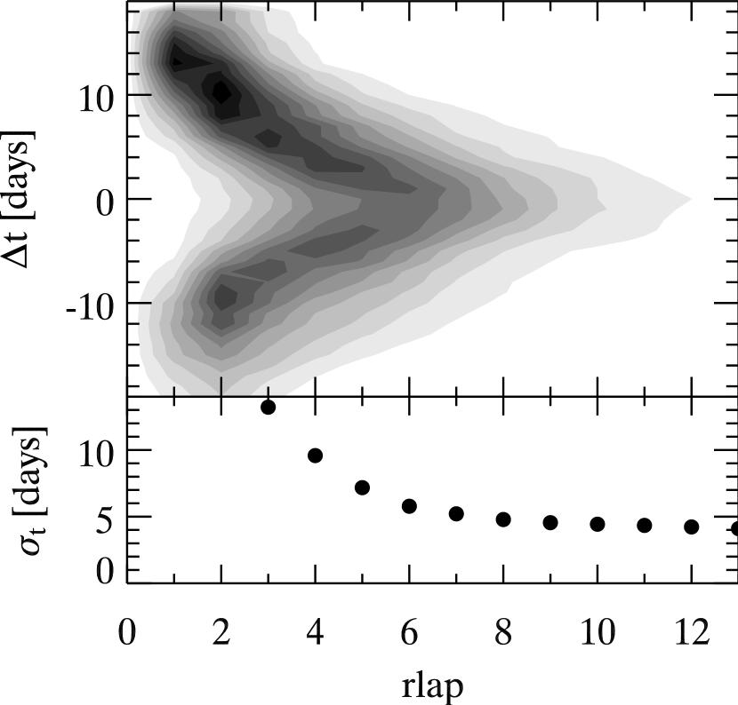
Figure 13.— Top: 2D histogram of age residuals vs. the $r{\rm lap}$ quality parameter (with ${\rm lap}\geq 0.4$), with the same parameters as in Fig. 9. The gray scale reflects the number of points in a given 2D bin (the more points the darker). Bottom: Standard deviation, $\sigma_{t}$, of age residuals in $r{\rm lap}$ bins of size unity. For $r{\rm lap}\gtrsim 6$, $\sigma_{t}\lesssim 5$ days.

The most striking feature in the gray scale of Fig. 13 is the near absence of points around $\Delta t=0$ for low values of $r{\rm lap}$. For poor correlations, the age is systematically mis-estimated, with a tendency to overestimate the age by $\sim 10$ days. Again, this is an artifact of the pseudo-continuum removal, which causes many maximum-light spectra to correlate with $\sim+10$-day templates (see § 5.2). It is also due to the nature of the supernova evolution, as the spectra evolve more rapidly around maximum light than they do around 10 days past maximum (Fig. 8), increasing the likelihood of correlations with templates at these ages.

There is no formal estimator for the age error. We have examined the distribution of age residuals above a certain $r{\rm lap}$ cutoff (cf. Fig. 12 for redshift) and find the median age of all templates with $r{\rm lap}\geq 5$ to be a good estimate of the spectral age. However, the standard deviation of all template ages with $r{\rm lap}\geq 5$ tends to systematically overestimate the age error by $\sim 20\%$.

5.4. Covariance Between Redshift and Age

The determination of redshift and age is intrinsically connected, and in principle one should marginalize over one parameter to infer the other. Marginalizing out the redshift (a continuous variable) to infer the age is straightforward, but the reverse is more complex, as it involves marginalization over sparsely sampled variables. The techniques to do this abound in the Bayesian literature, but we have yet to implement them in SNID. Nevertheless, we illustrate the covariance between redshift and age using the 2D histogram of age versus redshift residuals, for correlations satisfying $r{\rm lap}\geq 5$ (Fig. 14). As expected (see § 5.2), over(under)-estimating the age leads to under(over)-estimating the redshift, since the loci of maximum absorption shift to the red with age (Fig 10).

Figure 14.— Age residuals vs. redshift residuals, illustrating the covariance between the two quantities. We show the $1\sigma$ (solid line) and $2\sigma$ (dashed line) contours. The parameters are the same as those used in Fig. 9, with the requirement that $r{\rm lap}\geq 5$.

The anti-correlation between redshift and age residuals shown in Fig. 14 suggests that constraints on one parameter should improve the accuracy of the other. Fig, 15 shows the effect on the distributions of redshift (left panel) and age (right panel) residuals (for $r{\rm lap}\geq 5$; open histograms) of adding a flat $\pm 3$-day constraint on age and a flat $\pm 0.01$ constraint on redshift, respectively (hatched histograms). A constraint on the age leads to a $\sim 30\%$ narrower distribution of redshift residuals (from $\sigma_{z}=0.006$ to $\sigma_{z}=0.004$) and a constraint on redshift improves the age determination by $\sim 15\%$ ($\sigma_{t}=3.4$ days to $\sigma_{t}=2.9$ days). In practice, the constraint on redshift generally comes from a spectrum of the SN host galaxy and one can impose a constraint on age using a well-sampled light curve of the supernova (one for which the date of maximum light is easily determined).

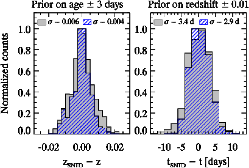
Figure 15.— Effect of age and redshift constraints on redshift (left) and age (right panel) residuals, respectively, with the same parameters as in Fig. 9. Here $z_{\rm{\rm SNID}}$ ($t_{\rm{\rm SNID}}$) corresponds to the median of all redshifts (ages) with $r{\rm lap}\geq 5$. The open and hatched histograms correspond to residuals with no constraint and a constraint on $(z,t)$, respectively. [See the electronic version of the Journal for a color version of this figure.]

The age distribution of SN spectral templates in the database affects the accuracy of both cross-correlation age and redshifts. In Fig. 16 we show the result of a Monte Carlo simulation where we compute the number of SN Ia spectra in bins of 3 days that would be sufficient for accurate redshift (left panel) and age (right panel) determinations with SNID. The solid histogram is the actual age distribution of normal SN Ia templates in the interval $-10\leq t_{B}\leq+20$ and the dotted histogram is the Monte Carlo distribution. We compute 1000 Monte Carlo realizations for each unity increment in the number of spectra in a given 3-day age bin. The number of spectra was chosen such that adding more spectra would not change the mean redshift and age residuals (for $r{\rm lap}\geq 5$) by more than 0.0001 and 0.1 days, respectively. For this Monte Carlo distribution, at least eight correlations with $r{\rm lap}\geq 5$ are needed for the median redshift and associated error (Fig. 12) to provide an accurate estimate.

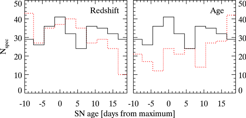
Figure 16.— Actual (solid line) and Monte Carlo (dotted line) age distributions of normal SN Ia templates for redshift (left panel) and age (right panel) determination. The Monte Carlo distribution was computed such that adding more spectra would not change the mean redshift and age residuals (for $r{\rm lap}\geq 5$) by more than 0.0001 and 0.1 days, respectively. [See the electronic version of the Journal for a color version of this figure.]

The Monte Carlo age distribution for redshift determination (Fig. 16, left panel) has an initial peak around $-10$ days and a bell-shaped envelope roughly centered around maximum ($0$ days)— akin in fact to a supernova light curve. This is due to the faster evolution of supernova spectra around maximum light than around 1–2 weeks past maximum (Figs. 8 & 10). In other words, SNID can accurately determine the redshift of an input spectrum at $+10$ days using a template at $+15$ days, since the wavelength (velocity) positions and relative strengths of spectral features change little over this age interval, but will be less accurate when an input spectrum at maximum light is correlated with template spectra at +5 days, since the evolution of the spectra is more significant then. The initial peak around $-10$ days is due to the rapid decrease in spectral line blueshifts from $\lesssim-10$ days to $\sim-5$ days (Fig. 10; Benetti et al. 2005; Blondin et al. 2006a), rather than to a change in the relative strengths of spectral features. We are currently lacking normal SN Ia spectral templates around +5 days past maximum light. This gap will be filled shortly with a new set of spectra from the CfA Supernova Program (almost 50 SNe Ia with more than 10 epochs of spectroscopy since 2000).

The Monte Carlo age distribution for age determination (Fig. 16, right panel) is altogether different, but the same reasons apply: due to the rapid evolution of SN spectra around maximum light, it is easier to accurately determine the age then than at 1–2 weeks past maximum, where the spectra evolve on longer timescales. Hence, more spectra are needed at later ages than around maximum light. The current number of normal SN Ia templates in our database is sufficient for accurate age determinations out to $t\lesssim+15$ days, but we need twice the number of templates in the last age bin. Again, this is within reach with the new set of CfA spectra.

To minimize the impact of our currently non-optimal age distribution of SN Ia templates, we have studied the redshift and age residual distribution when imposing a $1/N_{\rm temp}(t)^{a}$ weighting scheme, where $N_{\rm temp}(t)$ is the template age distribution (in 3-day bins) and $0.0\leq a\leq 2.0$ ($a=0.5$ corresponds to a Poisson-like weighting scheme). This way, the artificial attractors in the actual age distribution around maximum light and +10 days are down-weighted with respect to templates at other ages. The weighting scheme does not lead to any improvement in either the redshift or age determinations, namely the distribution of residuals for $r{\rm lap}\geq 5$ does not get any narrower. Clearly, a more elaborate method is necessary to break the redshift-age degeneracy and the covariance between the two quantities will be included explicitly in a future version of SNID.

Fig. 16 only shows the age distribution of normal SN Ia templates, for which we have sufficient spectra in the database to construct a viable Monte Carlo simulation. The faster evolution of supernova spectra around maximum light is common to all supernova types, but the homogeneity at a given age may vary significantly. We are not in a position to test this thoroughly, due to the limited number of Type Ib/c and Type II templates in the current SNID database. Again, we are confident that new data from the CfA Supernova Program will better constrain the variance of SN spectra at a given age (almost 20 SNe Ib/Ic/II with more than 10 epochs of spectroscopy since 2000). Therefore, while the overall shape of the Monte Carlo distributions should remain the same, the absolute scale should be different for the various supernova types.

5.5. Variation of Redshift and Age Accuracy with Redshift, Age, S/N and Galaxy Contamination

The previous studies are valid for the following parameter space: $0.3\leq z\leq 0.5$; $-5\leq t_{B}\leq+15$; $2\leq$ S/N (per 2 Å)$\leq 10$. However, we expect the accuracy of cross-correlation redshifts and ages to change with redshift, age and signal-to-noise ratio of the input spectrum.

In top panels of the left group of panels of Figure 17 we show the variation of the standard deviation of redshift residuals, $\sigma_{z}$, with the $r{\rm lap}$ quality parameter for varying redshift (left), age (middle), and S/N (right). We expect the degrading accuracy with redshift, since the rest-frame overlap (${\rm lap}$) between the input and template spectra in our database decreases with redshift. Even requiring that ${\rm lap}\geq 0.4$ can lead to degenerate redshifts at the higher end of the redshift range ($z\gtrsim 0.5$). Increasing the number of spectra extending blueward to $\lambda\gtrsim 2000$ Å would partially alleviate this problem, although the flux is strongly depleted at these wavelengths (due to line-blanketing from iron-group elements) and the most prominent features in supernova spectra are at optical wavelengths. UV spectra of (nearby) supernovae are rare, but the database could be expanded at these wavelengths (for SNe Ia, at least) by including the higher-S/N publicly-available spectra of ongoing high-$z$ SN searches, such as the spectra from the ESSENCE project (Matheson et al., 2005).

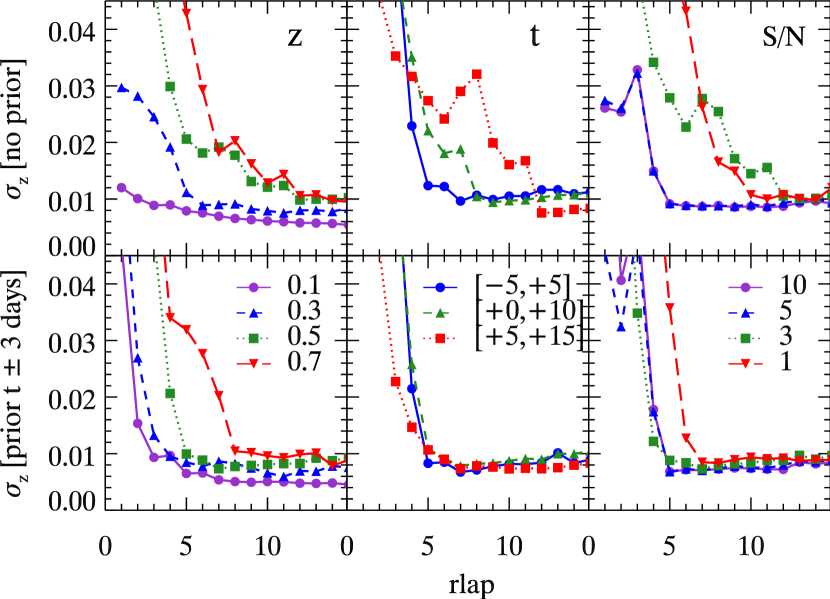
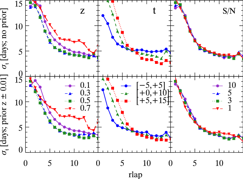
Figure 17.— Left: Variation of $\sigma_{z}$ with redshift (top left), age (in days; top middle) and S/N (per 2 Å; top right). We show the effect of applying a $\pm 3$ day constraint on age in the bottom panels. Right: Same as the left group of panels, but for the variation of $\sigma_{t}$ with redshift (top left), age (top middle) and S/N (top right). We show the effect of applying a $\pm 0.01$ constraint on redshift in the bottom panels. [See the electronic version of the Journal for a color version of this figure.]

The variation of $\sigma_{z}(r{\rm lap})$ with S/N of the input spectrum (Fig. 17, left group of panels; top right panel) is also expected, with a significant degradation below S/N $\lesssim 3$ per 2 Å. The degradation with increasing age of the input spectrum is again due to the slower evolution of SN spectra at later ages. The input spectrum will correlate well with template spectra over a larger range of ages, where the scatter in the velocity location of spectral features will translate directly into an error in redshift.

In the bottom panels of the left group of panels of Figure 17 we show the effect of applying a flat $\pm 3$ day age constraint on the $\sigma_{z}(r{\rm lap})$ curves. The improvement is significant in all cases (although less so for $z=0.7$).

In the top panels of the right group of panels Figure 17 we show the variation of the standard deviation of age residuals, $\sigma_{t}$, with the $r{\rm lap}$ quality parameter for varying redshift (left), age (middle), and S/N (right). Again, the degradation at the highest redshift ($z=0.7$) is expected, although it is surprising that the $\sigma_{t}(r{\rm lap})$ curves for $z=0.3$ and $z=0.5$ lie atop the one corresponding to $z=0.1$. It appears that the optimal rest frame wavelength range of the input spectrum is different for redshift and age determination. This has already been mentioned by Foley et al. (2005) concerning the age determination and points towards the need for an age- and wavelength-dependent ${\rm lap}(t,\lambda)$ parameter to weight the correlation height-noise ratio, $r$, instead of the constant ${\rm lap}$ currently implemented in SNID. The difficulty of determining the age of an input spectrum at later times is due to the less rapid evolution of the spectra at these ages. At high values of $r{\rm lap}$ ($\gtrsim 7$), however, $\sigma_{t}$ decreases with age. This behavior is unexpected, given the discussion in § 5.4 and could again be due to the wavelength-independent nature of our ${\rm lap}$ parameter.

Even more surprising is the apparent independence of $\sigma_{t}(r{\rm lap})$ on S/N: for fixed redshift and age (here $z=0.5$ and $-5\leq t_{B}\leq+5$), the $r{\rm lap}$ quality parameter gives an absolute measure of the age accuracy, regardless of the S/N of the input spectrum. Of course, the probability of having correlations with high $r{\rm lap}$ values drops with S/N, but we have checked that our simulation yielded a sufficient number of correlations at $r{\rm lap}\gtrsim 7$ for this result to be statistically significant.

We next study the impact of contamination from the underlying spectrum of the host galaxy affecting the input supernova spectrum. The contamination fraction will depend both on the projected position of the supernova within its host (higher contamination closer to the nucleus) and on the relative flux difference between the supernova and the portion of the galaxy located in the same aperture (i.e. immediately underlying the SN trace, when extracting the spectrum). Several techniques are commonly used to separate the supernova light from that of the host galaxy, either through galaxy template subtraction (e.g., in the algorithm presented by Howell et al. 2005), or using more elaborate techniques such as two-channel deconvolution directly applied to the 2D spectrum (Blondin et al., 2005). However, neither of these techniques works well in cases where the SN lies on top of the nucleus of a bright galaxy and in all other cases there still remains some fraction of galaxy light in the SN spectrum.

We contaminate each input spectrum in our simulation with galaxy light, using the elliptical and Sc galaxy templates of Kinney et al. (1996). The top panels of Figure 18 show the effect on redshift residuals, $\sigma_{z}(r{\rm lap})$, of increasing the galaxy contamination fraction (expressed in fractions of the total flux) from 0.00 to 0.50. The impact of the elliptical galaxy (top left panel) is most severe, since the spectra of early-type hosts contain broad continuum structures that yield strong power at similar wavenumbers as supernova features in Fourier space. Late-type galaxies have smoother continua and their narrow emission lines are filtered out using the bandpass filter. In the bottom panels of Fig. 18 we apply a flat age constraint of $\pm 3$ days. The improvement, if any, is negligible for both the elliptical and Sc galaxy types.

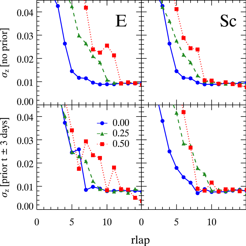
Figure 18.— Top: Impact of galaxy contamination fraction on $\sigma_{z}(r{\rm lap})$, for both elliptical (E; left panel) and spiral (Sc; right panel) galaxies. The different lines correspond to different galaxy contamination fractions, expressed in fractions of the total flux. Bottom: Effect of applying a $\pm 3$-day constraint on the age. [See the electronic version of the Journal for a color version of this figure.]

We have run several simulations to test whether the $r{\rm lap}$ quality parameter could be used to evaluate the amount of galaxy contamination for various galaxy types, but the results were inconclusive. This constitutes the real limit of SNID: some extra pre-processing of the supernova spectrum is necessary to ensure that the input to SNID is as “clean” as possible. Other algorithms (see § 7) perform a simultaneous fit of the galaxy fraction when comparing the input SN spectrum to the set of templates in the database, which enables the classification of supernovae when the galaxy contamination is $\lesssim 75\%$ (Howell et al., 2005).

5.6. Comparison with External Measurements

In this section we test the accuracy of correlation redshifts using SNID by comparing them with those of the host galaxy. Galaxy redshifts ($z_{\rm GAL}$) are routinely determined using nebular emission lines in their spectra or by cross-correlation with absorption-line galaxy spectral templates (Kurtz & Mink, 1998). They are typically accurate to $<0.001$. However, the redshift of the supernova can differ from $z_{\rm GAL}$, since the supernova event may have occurred in a region where its velocity (in the galaxy rest frame) is different from the mean value, due to the velocity dispersion of the galaxy’s light-emitting component ($\sim 100$ km s^-1 and $\sim 200$ km s^-1 in early- and late-type galaxies, respectively; McElroy 1995). Nevertheless, $z_{\rm GAL}$ gives a more accurate determination of the SN redshift than SNID (which has typical redshift errors of $\lesssim 0.01$ for $r{\rm lap}\geq 5$), so a comparison of the two gives a valuable indication on the accuracy of SNID redshifts, determined from real data.

We have selected high-redshift SN Ia spectra taken by the ESSENCE team (Matheson et al. 2005; Foley et al., in prep; Blondin et al., in prep), for which a redshift of the host galaxy was obtained. This amounts to 57 SN Ia spectra in the redshift range $0.164\leq z\leq 0.782$. The result of this comparison is shown in the left panels of Figure 19. The dispersion about the one-to-one correspondence of the redshifts is excellent, with $\sigma_{z}\approx 0.005$ over the whole redshift range. This is in good agreement with the expected redshift residual found from simulations (with no constraint on the age; Fig. 15). The bottom left panel shows a plot of the redshift residuals as a function of the galaxy redshift. The mean residual is $\sim 4\times 10^{-4}\ll\sigma_{z}$, which shows that there are no systematic effects in using SNID to determine the SN redshift.

Figure 19.— Left: Comparison of redshifts determined from cross-correlations with SN Ia spectral templates using SNID ($z_{\rm{\rm SNID}}$) and from narrow lines in the host galaxy spectrum ($z_{\rm GAL}$; top). We show the residuals vs. $z_{\rm GAL}$ in the bottom panel. Right: Comparison of supernova spectral ages determined using SNID ($t_{\rm{\rm SNID}}$) and rest-frame light-curve ages ($t_{\rm LC}$) of high-$z$ SNe Ia ($0.164\leq z\leq 0.587$; top). We show the residuals vs. $t_{\rm LC}$ in the bottom panel. The data are from the ESSENCE project (Matheson et al. 2005; Miknaitis et al. 2007; Foley et al., in prep; Blondin et al., in prep).

To compare the supernova age determined through cross-correlation with external measurements, we select ESSENCE high-redshift SN Ia spectra for which a well-sampled light curve is available around maximum light (Miknaitis et al., 2007). This way we can determine the time difference (in the observer frame) between maximum light, ($t_{\rm max}$) and the time the spectrum was obtained ($t_{\rm spec}$) and compare this time interval with the rest-frame age ($t_{\rm{\rm SNID}}$) determined through cross-correlation with local SN Ia templates. For this comparison to make sense we must correct the light-curve age for the $(1+z)$ time-dilation factor expected in an expanding universe (Wilson, 1939; Rust, 1974; Leibundgut et al., 1996; Goldhaber et al., 2001). We expect a one-to-one correspondence between

$$t_{\rm LC}=\frac{t_{\rm spec}-t_{\rm max}}{1+z}$$ (22)

and $t_{\rm{\rm SNID}}$. The result is shown in the right panels of Figure 19. We used a total of 54 spectra in the redshift range $0.205\leq z\leq 0.687$, 27 of which had an associated galaxy redshift— which we used as a constraint when determining the age. The dispersion about the $t_{\rm{\rm SNID}}=t_{\rm LC}$ line is $\sigma_{t}\approx 2.9$ days over a age interval $-10\lesssim t_{\rm LC}\lesssim+20$, again in good agreement with the expected residuals (Fig. 15). We show the residuals versus $t_{\rm LC}$ in the bottom right panel. The mean residual is approximately $-0.7$ days. The excellent correspondence between $t_{\rm LC}$ and $t_{\rm{\rm SNID}}$ shows that SNID can be used in studies of time dilation effects in high-redshift multiepoch SN Ia spectra (Riess et al., 1997; Foley et al., 2005).

The correlation technique could not have yielded such good results had the high-$z$ SNe Ia in the sample been significantly different from the SN Ia template spectra in the SNID database. The fact that the correlation redshifts and ages agree so well with the galaxy redshifts and light-curve ages, respectively, is a strong argument in favor of the similarity of these SNe Ia with local counterparts.

6. Type Determination

The results of § 5 are only valid if we assume that we know the type of the input supernova spectrum— in this case a normal SN Ia. Although SNID is tuned to determining SN redshifts, we investigate its potential in determining the SN type in an impartial way. We base our investigation on a simple frequentist approach as opposed to a more elaborate Bayesian one, but we discuss the future implementation of the latter in SNID in § 7.

In what follows we focus on five distinct examples, the first three being particularly relevant to ongoing high-redshift SN Ia searches: the distinction between 1991T-like SNe Ia and other SNe Ia (§ 6.1); the distinction between SNe Ib/c and SNe Ia at high redshifts (§ 6.2); the identification of peculiar SNe Ia (§ 6.3); finally, the distinction between SNe Ib and SNe Ic and between SNe IIb and both SNe II and Ib (§ 6.4), more relevant to ongoing nearby ($z\lesssim 0.1$) supernova searches. We used the same simulation setup as in § 5.1, except we consider correlations with all supernova types in the database.

The reader must keep in mind that, while the age distribution of SN Ia templates is close to optimal in the current SNID database (see § 5.4), those for supernovae of other types are most certainly not. While the results presented in this section are encouraging, they are no doubt biased by the relatively low number of SN Ib/Ic/II templates with respect to SNe Ia.

6.1. Normal versus 1991T-like SNe Ia

It can be challenging to distinguish the subtypes of SNe Ia from one another. 1991T-like SNe Ia have a peak luminosity at the bright end of the SN Ia distribution and although their light curves still obey the width-peak luminosity, or “Phillips,” relation (Phillips, 1993), it is useful to have an independent confirmation of their high intrinsic luminosity from their spectra. Spectra of 1991T-like SNe Ia are characterized by the near-absence of Ca ii and Si ii lines in the early-time spectra, and prominent high-excitation features of Fe iii— not found in normal SNe Ia. The Si ii, S iiand Ca ii features develop during the post-maximum ages and by $\sim 2$ weeks past maximum the spectra of “1991T-like” objects are similar to those of normal SNe Ia (Filippenko et al., 1992; Ruiz-Lapuente et al., 1992; Phillips et al., 1992; Jeffery et al., 1992).

In the top panels of Figure 20 we illustrate the ability of SNID to identify 1991T-like SNe Ia at $z=0.5$. The input spectrum is a “Ia-91T” template in the SNID database (Table Determining the Type, Redshift, and Age of a Supernova Spectrum) in the age interval $-5\leq t_{B}\leq+5$, i.e. when the spectroscopic differences with normal SNe Ia are most apparent. We show the fraction of templates in the SNID database that correlate with the input spectrum, as a function of the $r{\rm lap}$ quality parameter: 1991T-like SNe Ia (solid line), other SNe Ia (dashed line), and supernovae of other types (dotted line). From left to right, we show the effect of having no constraint on either age or redshift, a flat $\pm 0.01$ constraint on redshift, a flat $\pm 3$ day constraint on the age, and a combined constraint on both redshift and age.

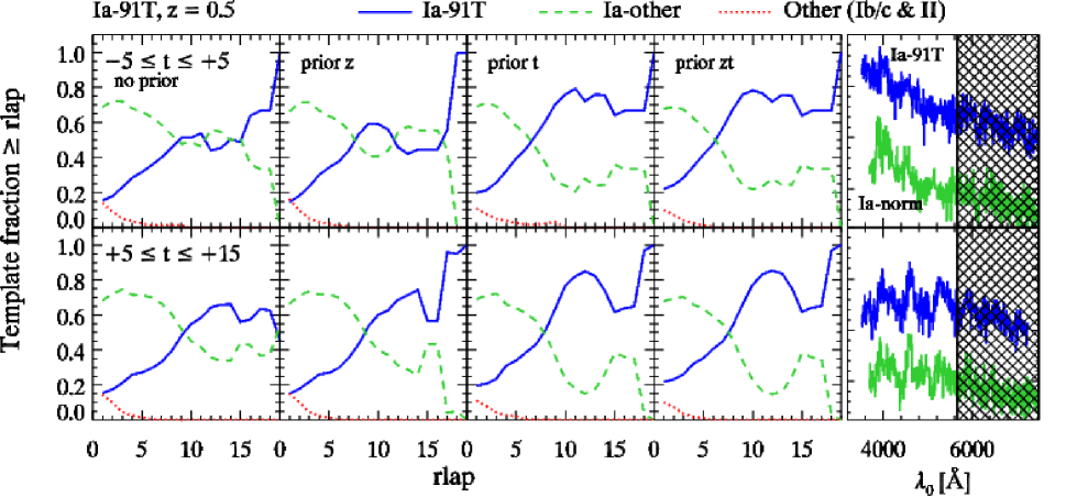
Figure 20.— Attempt to identify a 1991T-like SN Ia at $z=0.5$ in the age interval $-5\leq t_{B}\leq+5$. Top: Fraction of templates in the SNID database corresponding to a certain supernova type (1991T-like SN Ia: solid line; SN Ia of other subtypes: dashed line; supernova of other types: dotted line), in $r{\rm lap}$ bins of size unity. Left to right: With no constraints on the redshift or age, with a $\pm 0.01$ constraint on the redshift, with a $\pm 3$ days constraint on the age, and with a combined constraint on redshift and age. Bottom: Same lines as above, but for post-maximum spectra in the age interval $+5\leq t_{B}\leq+15$. The right panel shows representative spectra of 1991T-like and normal SNe Ia, around maximum light (top) and $\sim$1–2 weeks past maximum (bottom), as observed with a typical optical spectrograph at $z=0.5$ (the cross-hatched area represents the rest frame portion of the spectrum that is lost due to the redshift). Note that the relative differences in pseudo-continuum shapes have no impact on the SNID results. [See the electronic version of the Journal for a color version of this figure.]

When there is no constraint on either redshift or age, the fraction of Ia-91T templates (solid line) for $r{\rm lap}\gtrsim 10$ is greater than that for other SN Ia templates (dashed line). Note that for $r{\rm lap}\gtrsim 5$ the confusion with supernovae of other types is practically non-existent ($\lesssim 2\%$). Adding a constraint on the redshift does not lead to a significant improvement, but a constraint on age reduces the cross-over $r{\rm lap}$ value between other SN Ia and 1991T-like templates from $r{\rm lap}\gtrsim 15$ to $r{\rm lap}\approx 6$. The negative noise spikes around $r{\rm lap}\approx 15$ are statistical noise due to the small number of templates with $r{\rm lap}$ values in excess of that cutoff.

The bottom panels of Figure 20 show the same lines for input spectra in the age interval $+5\leq t_{B}\leq+15$. At these post-maximum ages, the differences between 1991T-like and normal SNe Ia are less apparent (see the rightmost panel) and the impact on the ability of SNID to distinguish between the different Ia subtypes is readily apparent. In the absence of constraints on redshift or age, the fraction of Ia-91T templates reaches a peak of $\sim 70$%, while it increases to 100% with constraints on redshift and age. The variation for $r{\rm lap}\geq 15$ is again statistical noise due to the limited number of templates with such good correlations.

The difficulty of distinguishing between normal and 1991T-like SNe Ia at high redshift could partly explain the apparent lack of 1991T-like SNe Ia at high redshifts ($2/52\approx 4$% in the SN Ia sample published by Matheson et al. 2005) with respect to the fraction expected locally (up to $\sim 20$% according to Li et al. 2001b).

6.2. SN Ia versus SN Ib/c

The misidentification of supernovae of other types as SNe Ia is a major concern for ongoing high-redshift SN Ia searches. Including only a small fraction of non-Ia supernovae in a sample would lead to a mis-calibration of the absolute magnitudes of these objects and to biases in the derived cosmological parameters (Homeier, 2005). A particular concern is the contamination of high-z SN Ia samples with SNe Ib/c. At redshifts $z\gtrsim 0.4$, the defining Si ii $\lambda 6355$ absorption feature of SNe Ia (also present, although somewhat weaker, in SNe Ic) is redshifted out of the range of most optical spectrographs and one has to rely on spectral features blueward of this to determine the supernova type. Some of these features, such as the Ca ii H and K $\lambda\lambda 3934,3968$ doublet, are common to both SNe Ia and SNe Ib/c. Other features characteristic of SN Ia spectra around maximum light (e.g. S ii $\lambda\lambda 5454,5640$) are generally weak and can be difficult to detect in low-S/N spectra. One has to invoke external constraints, such as the SN color evolution, light-curve shape, host galaxy morphology (only SNe Ia occur in early-type hosts; Cappellaro et al. 1997), or the expected apparent peak magnitude: SNe Ib/c at maximum light are often $\gtrsim 1$ mag fainter than SNe Ia (Richardson et al. 2006; although Clocchiatti et al. 2000 have reported on one SN Ic with an absolute magnitude similar to normal SNe Ia) and hence are only expected to “pollute” magnitude-limited samples of SNe Ia at the lower-redshift end. If the redshift is not known, SNe Ib/c can be a serious contaminant for high-redshift SN Ia searches.

In the top panels of Figure 21 we illustrate the ability for SNID to identify SNe Ib/c at $z=0.3$. The input spectrum is a “Ib-norm” or “Ic-norm” template in the SNID database (Table Determining the Type, Redshift, and Age of a Supernova Spectrum) in the age interval $-5\leq t_{B}\leq+5$. We show the fraction of templates in the SNID database that correlate with the input spectrum, as a function of the $r{\rm lap}$ quality parameter: all SNe Ib/c (including SNe IIb; solid line), SNe Ia (dashed line), and SNe II (excluding SNe IIb; dotted line).

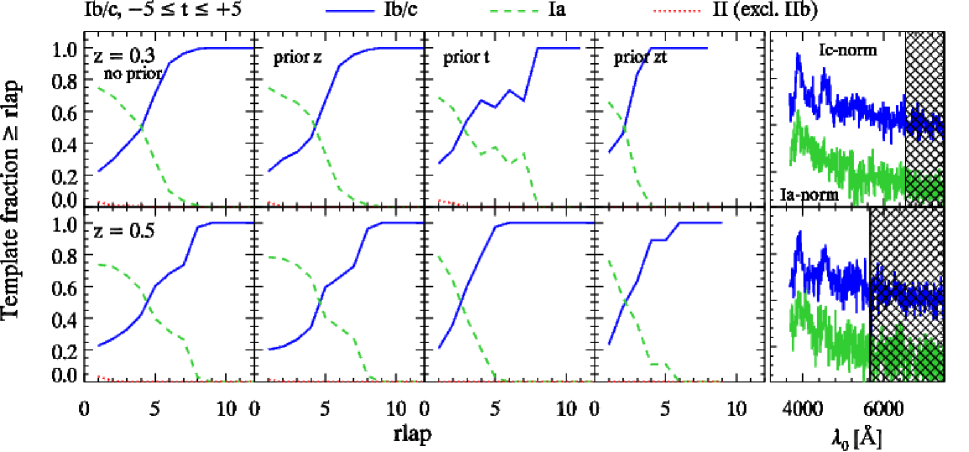
Figure 21.— Same as Fig. 20, but for normal SNe Ic in the age interval $-5\leq t_{B}\leq+15$, at $z=0.3$ (top) and $z=0.5$ (bottom). Here the lines correspond to fractions of SNe Ib/c (solid line), SNe Ia of all subtypes (dashed line), and SNe II (excluding SNe IIb, dashed line). [See the electronic version of the Journal for a color version of this figure.]

In the absence of a constraint on age, correlations with $r{\rm lap}\gtrsim 4$ are sufficient to recover a dominant fraction of SNe Ib/c over SNe Ia. The confusion with SNe II is practically nonexistant ($<5\%$ for $r{\rm lap}\lesssim 3$; 0% for $r{\rm lap}>3$). A constraint on age only reduced the cross-over $r{\rm lap}$ between SNe Ia and SNe Ib/c from $r{\rm lap}\approx 4$ to $r{\rm lap}\approx 3$ but leads to less correlations with $r{\rm lap}\gtrsim 5$ (hence the noise spikes in the recovered template fractions). A combined constraint on redshift and age yields a 100% SN Ib/c fraction for $r{\rm lap}\geq 4$, but no correlations with $r{\rm lap}>8$.

At $z=0.5$, the results are essentially unchanged from $z=0.3$, although the absolute number of good correlations ($r{\rm lap}\gtrsim 5$) is generally less. We also note that these results are biased by the confusion between SNe Ib and SNe Ic at this redshift (up to $\sim 40\%$). The constraint on age leads to a more significant improvement than at $z=0.3$, suggesting that the similarity between spectra of SNe Ic around maximum light and SNe Ia at $\sim$1–2 weeks past maximum is less problematic over this restricted wavelength range.

Note that the mis-classification of SNe Ib/c as SNe Ia (or the reverse) can sometimes pose problems with the high-S/N spectra of nearby objects, especially at later ages or if no age information is available. A striking example is the nearby SN Ic SN 2004aw (Taubenberger et al., 2006), originally classified as an SN Ia by Benetti et al. (2004). More recently, two nearby supernovae originally announced as Type Ic events around maximum light (SN 2006bb and SN 2006bk; Kinugasa & Yamaoka 2006a, b) were re-classified as SNe Ia at 2–3 weeks past maximum light based on cross-correlations with SN spectra of all types using SNID (Blondin et al., 2006b, c).

6.3. Identifying SN Ia “Oddballs”

Some SNe Ia, which we refer to as peculiar, do not belong to any of the normal, 1991T-like, or 1991bg-like categories. Such is the case of SNe 2000cx (Li et al., 2001a), 2002cx (Li et al., 2003) and 2005hk (Phillips et al., 2007). The first of these has pre-maximum spectra similar to those of SN 1991T, although the Si ii lines that appear around maximum light remain strong several weeks past maximum. SN 2002cx, “the most peculiar known SN Ia” (Li et al., 2003; Branch et al., 2004; Jha et al., 2006b) and SN 2005hk are even more difficult to accommodate in the current classification scheme: their early-time spectra show signatures of high-ionization lines of iron, as in the overluminous SN 1991T, but their luminosity is similar to that of the subluminous SN 1991bg. Moreover, their $I$-band light curves are devoid of the secondary maximum present in all other Ia subtypes. Both objects possibly originate from a pure deflagration explosion (see Phillips et al. 2007) and could form an altogether separate class of SNe Ia.

These peculiar SNe Ia do not obey the Phillips relation and thus cannot be used as calibrated distance indicators. They must be weeded out of high-redshift SN Ia samples in order to avoid significant biases in the derived cosmological parameters. Until recently, there was no evidence for such peculiar events at high redshifts. This has changed with the recent discovery of the overluminous SNLS-03D3bb (SN 2003fg) at $z=0.244$ (Howell et al., 2006).

In the top panels of Figure 22 we illustrate the ability of SNID to identify peculiar SNe Ia at $z=0.3$. The input spectrum is a “Ia-pec” template in the SNID database (Table Determining the Type, Redshift, and Age of a Supernova Spectrum) in the age interval $-5\leq t_{B}\leq+5$. We show the fraction of templates in the SNID database that correlate with the input spectrum, as a function of the $r{\rm lap}$ quality parameter: peculiar SNe Ia (solid line), other SNe Ia (dashed line), and supernovae of other types (dotted line). In the absence of a constraint on redshift, the maximum recovered fraction of Ia-pec templates is $\sim 5$%, with no correlations at $r{\rm lap}>6$. With a constraint on redshift, the Ia-pec template fraction peaks at $\sim 70$%, but the best correlations are always for another Ia subtype (most frequently 1991T-like). At $z=0.5$, the recovered fraction of Ia-pec templates is complete for $r{\rm lap}\geq 5$ for both a constraint on redshift and a combined constraint on redshift and age. This apparent improvement is counterbalanced by the absence of correlations with $r{\rm lap}>9$. Note that in the absence of any constraint, the recovered fraction of Ia-pec templates is dominant for $r{\rm lap}\gtrsim 6$.

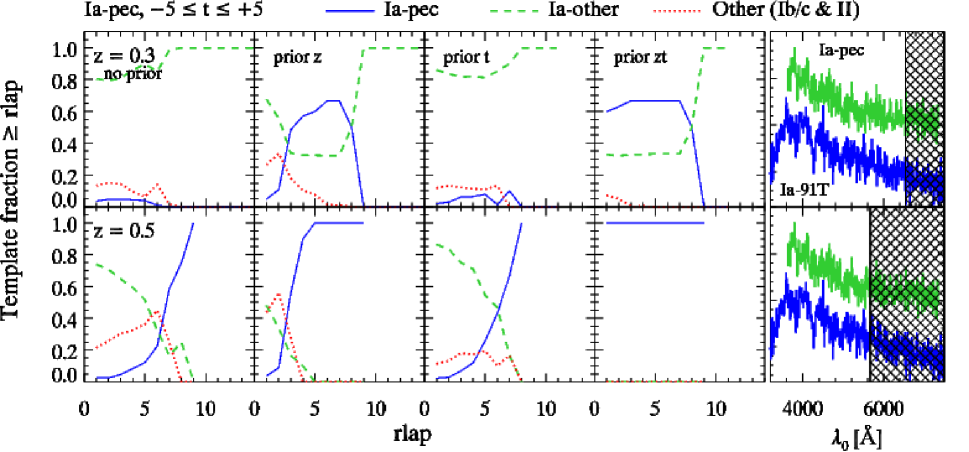
Figure 22.— Same as Fig. 20, but for a peculiar SN Ia in the age interval $-5\leq t_{B}\leq+15$, at $z=0.3$ (top) and $z=0.5$ (bottom). Here the lines correspond to fractions of peculiar SNe Ia (solid line), other SNe Ia (dashed line), and all other supernova types (dashed line). [See the electronic version of the Journal for a color version of this figure.]

Despite the limited number of peculiar SNe Ia in our database (SN 2000cx, SN 2002cx and SN 2005hk, for a total of 15 spectra in the age interval $-5\leq t_{B}\leq+5$; see Table Determining the Type, Redshift, and Age of a Supernova Spectrum), the change in template fraction from $z=0.3$ to $z=0.5$ gives indications as to which rest frame wavelength range is most valuable for determining the SN type. This again calls for a wavelength (and age) weighting of the spectrum overlap parameter, ${\rm lap}(\lambda,t)$ (see § 5.5), which we are working to implement in a future version of SNID.

We note that SNID unambiguously confirms the similarity between SN 2005hk and SN 2002cx (see Phillips et al. 2007): for all the spectra of SN 2005hk in the SNID database (Table Determining the Type, Redshift, and Age of a Supernova Spectrum), the best-match template spectrum is SN 2002cx, whether a constraint on redshift and age is applied or not. In the absence of a constraint on redshift, however, the fraction of 1991T-like templates that correlate with the input SN 2005hk spectrum increases dramatically, leading to an overestimation of the redshift by $\sim 0.02$, roughly corresponding to the difference in absorption velocities between SN 2005hk and SN 1991T at a given age ($\sim 6000$ km s^-1; Phillips et al. 2007).

SNLS-03D3bb (SN 2003fg) at $z=0.244$ (Howell et al., 2006), on the other hand, illustrates the limitations of the cross-correlation approach in determining the SN type, when applied to objects that are not part of the library of spectral templates. Its spectrum (at +2 days; A. Howell, private communication) is unique among supernova spectra and we have no similar examples in our database. In the absence of constraints, the best-match template is the 1991T-like SN 1999dq (Matheson et al., 2007) at $t=+6.2$ days ($z=0.254\pm 0.005$). With constraints on age or redshift, the best-match template is in all cases the normal SN Ia SN 1989B at $t=+3.5$ days ($z=0.251\pm 0.005$). The spectrum of SNLS-03D3bb is now part of the SNID database and will prove useful to identify such peculiar objects at all redshifts.

6.4. Further Specific Examples

We next focus on two further specific examples, relevant to the spectroscopic classification of supernovae in nearby ($z\lesssim 0.1$) SN searches: the distinction between SN Ib and Ic, and that between SN IIb and II/Ib.

6.4.1 SN Ib versus SN Ic

SN Ib and Ic are often difficult to tell apart and are sometimes referred to as “SNe Ib/c” in the literature (e.g., SN 1999ex; Hamuy et al. 2002) and IAU circulars. This difficulty is inherent to the SN classification scheme, rather than from a physical mis-conception of these events, both of which are believed to originate in the core collapse of a massive star, stripped of its outer layers through either stellar winds or interaction with a binary companion (Woosley et al., 1993, 1995). SNe Ib are defined by the presence of conspicuous lines of He i in their optical spectra, whereas SNe Ic are defined by their quasi-absence (Matheson et al., 2001). The Si ii $\lambda$6355 feature is weak in SNe Ib/c, which enables one to differentiate them from SNe Ia, at least in principle (see § 6.2). Both are of Type I and are thus also defined by the absence of hydrogen lines in their spectra, although the case has recently been made for some hydrogen being present in SNe Ib/c (Branch et al., 2006; Elmhamdi et al., 2006).

In Fig. 23, we show the result of cross-correlating SN Ib spectra at low redshift ($z=0.1$) within 10 days from $V$-band maximum with SNe of all types in the SNID database: Type Ib (excluding Type IIb; solid line), Type Ic (dashed line), and other SN types (dotted line). The lines correspond to the fraction of template supernovae of a given type, as a function of the $r{\rm lap}$ quality parameter. We deliberately exclude the IIb subtype from this analysis, as this type is a hybrid between the II and Ib subtypes (see below). The results of Fig. 23 are encouraging: for $r{\rm lap}>6$, the recovered fraction of SN Ib dominates over SNe Ic, with less than 25% confusion with other supernova types. For $r{\rm lap}\geq 13$, only Type Ib templates correlate with the input spectrum.

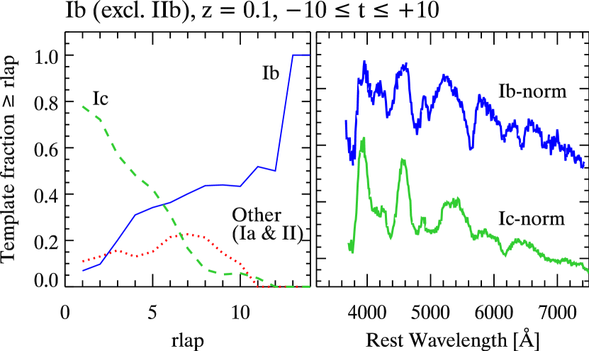
Figure 23.— Attempt to classify an SN Ib at $z=0.1$ in the age interval $-10\leq t_{V}\leq+10$. The lines correspond to fractions of matching templates of Type Ib (solid line), Type Ic (dashed line) and all other types (dotted line), in $r{\rm lap}$ bins of size unity. The Type IIb subclass, included in both the SN Ib and SN II categories, is excluded for this purpose. The right panel shows representative spectra of normal SN Ib and Ic around maximum light. Note that the relative differences in pseudo-continuum shapes have no impact on the SNID results. [See the electronic version of the Journal for a color version of this figure.]

6.4.2 SN IIb versus SN II/Ib

Some supernovae “evolve” from one type to another as they age. Such is the case for SNe IIb (Woosley et al., 1987), whose early-time spectrum is characterized by prominent P Cygni lines of the hydrogen Balmer series (as in SNe II), but which later develop conspicuous lines of He i, as in SNe Ib. A proto-typical example of such a supernova is SN 1993J (Nomoto et al., 1993; Matheson et al., 2000). The SNID database currently contains spectra for three SNe IIb: SN 1993J, SN 2000H and SN 2006T (Table Determining the Type, Redshift, and Age of a Supernova Spectrum).

In Fig. 24 we study the fraction of templates corresponding to Type IIb (solid line), Type II (dashed line), and Type Ib (dotted line), when the input spectrum is a Type IIb at low redshift ($z=0.1$), within 15 days past explosion. At these ages, the He i lines are somewhat weaker than after maximum and the confusion with SNe II is greater: only for $r{\rm lap}\gtrsim 7$ is the fraction of recovered IIb templates greater than ordinary SNe II. The confusion with Type Ib templates is small ($<20\%$) up to $r{\rm lap}\approx 9$ and null for larger values of $r{\rm lap}$. Templates corresponding to SNe Ia and Ic do not correlate well with input Type IIb spectra and the confusion is practically nonexistent ($<5\%$, not shown here). Again, more SNe IIb are needed to truly test the ability for SNID to correctly identify them.

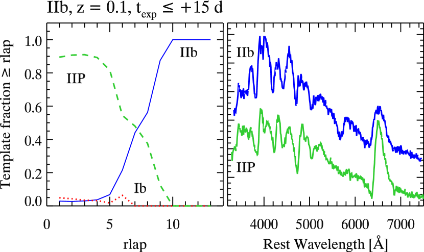
Figure 24.— Same as Fig. 23, but for an SN IIb at $z=0.1$ in the age interval $t_{\rm exp}\leq+15$ ($t_{\rm exp}$ is the number of days past explosion). The lines correspond to fractions of matching templates of Type IIb (solid line), Type II (dashed line) and Type Ib (dotted line), in $r{\rm lap}$ bins of size unity. [See the electronic version of the Journal for a color version of this figure.]

6.5. Using SNID for SN Identification

The previous examples illustrate the ability of SNID to recover a significant fraction of supernovae in the database corresponding to the input SN type. While Figs. 20–24 are informative, they do not provide a unique answer to the following: how does one use SNID to determine the type of an SN spectrum and can one relate the $r{\rm lap}$ quality parameter to a formal confidence that an input spectrum is of a certain type (and, sometimes more importantly, that it is not of another type)? The answer is far from settled, and its resolution will probably involve a more sophisticated Bayesian approach (see next section). Nevertheless, we have tested the following classification schemes:

• The SN type (subtype) is simply determined as the type (subtype) of the best-match template(s) for $r{\rm lap}$ greater than some cutoff value $r{\rm lap}_{\rm min}$.

• The SN type (subtype) is the one corresponding to the highest fraction of templates corresponding to a given type (subtype) for $r{\rm lap}\geq r{\rm lap}_{\rm min}$, with the possible additional requirement that this fraction exceeds some cutoff.

• The SN type (subtype) is the one whose fraction increases most with increasing $r{\rm lap}$ (i.e. the lines shown in Figs. 20–24 that have the highest positive gradient for $r{\rm lap}\geq r{\rm lap}_{\rm min}$), with the possible additional requirement that this gradient exceeds some cutoff.

The first of these is the one commonly used for the identification of supernovae, at both low and high redshift. In IAU circulars, a supernova is announced to be of a given type when it is “(most) similar to supernova $X$ at $N$ days from maximum light.” In high-$z$ SN Ia searches, a secure type is determined when a given spectrum is sufficiently similar to a nearby SN Ia (e.g., Matheson et al. 2005), but it is never clear how different it is from supernovae of other types. However, the best-match template is not always the best indicator of the SN type (see the distinction between post-maximum spectra of 1991T-like SNe Ia and other SNe Ia in Fig. 20) and the large spectral database used in SNID offers the possibility to use the statistical power of correlations exceeding a certain $r{\rm lap}$ cutoff. This second classification scheme has already been used for the classification of high-$z$ SN Ia spectra using SNID (Miknaitis et al., 2007). A drawback of such an approach is that the determination of the SN type depends on the completeness of the SN database— which comprises few template spectra of core-collapse SNe (Ib,Ic, and II; see § 4). Thus, for instance, it is not possible to identify peculiar SNe Ia this way (Fig. 22). Last, the “gradient method” for classification is generally more robust, but also requires some other constraint on either the template fraction or the type of the best-match template(s).

We are extensively testing these different combinations, to optimize the type determination for all SN types, at varying $z$, $t$, and S/N, although we suspect that a more elaborate Bayesian treatment will be required to properly account for the probability of an input spectrum to be of a certain type (as well as not being of some other type).

7. Comparison with Other Methods and Further Improvements

Several other methods are used to determine the type, redshift, or age of a supernova spectrum. We briefly describe them here, with a distinction between cross-correlation and “$\chi^{2}$-based” methods. Last, we comment on the alternative Bayesian approach to supernova classification— only applied so far to photometric measurements and its possible implementation in SNID.

Other spectral classification methods involve principle component analysis (PCA), possibly in combination with artificial neural networks. These are beyond the scope of this paper and we do not discuss them here, although the PCA method has already been applied to SN Ia classification by James et al. (2006).

7.1. Cross-correlation Methods

We are aware of two other algorithms based on the cross-correlation techniques of Tonry & Davis (1979). Both are aimed at determining redshifts of galaxies (or stars) in large surveys, but could easily be tuned (e.g., by modifying the shape of the bandpass filter and including age information) to supernovae as in SNID.

XCSAO (Kurtz & Mink, 1998) is a program part of the IRAF RVSAO package, aimed at obtaining redshifts and radial velocities from digital spectra. It has been used extensively in the past for redshift surveys (for references see Kurtz & Mink 1998) and is currently used in the Smithsonian Hectospec Lensing Survey (SHELS; Geller et al. 2005). The basic algorithm is the same as that described in § 2, although some important differences exist. First, the overlap in wavelength between the input and template spectra at the correlation redshift (the ${\rm lap}$ parameter discussed in § 3.2) is not taken into account explicitely; rather it is maximized by including spectral templates at different redshifts. Second, XCSAO directly selects the best peak in the correlation function, rather than looking at the 10 best peaks individually. Last, the reported correlation redshift is that associated with the best-match template (i.e., the one with the highest correlation height-noise ratio, $r$), rather than being the median of all redshifts above a certain cutoff $r_{\rm min}$. It may be that not including the ${\rm lap}$ parameter is less important for galaxy redshift determination, due to the narrower widths of spectral lines in galaxy spectra and the iterative scheme implemented in XCSAO ensures that an optimal correlation redshift is computed (D. Mink 2007, private communication). For supernova spectra, however, the inclusion of the ${\rm lap}$ parameter is fundamental to obtain reliable redshifts (see § 5.2). The other two differences are of a less fundamental nature.

Another algorithm based on the correlation techniques of Tonry & Davis (1979) is RUNZ (Saunders et al., 2004), a program used by members of the 2dF Galaxy Redshift Survey (Colless et al., 2001) and the 6dF Galaxy Survey (Jones et al., 2004). An essential difference with SNID is the scaling of the input spectrum by its inverse-variance (see § 2.2), which leads to improved cross-correlation redshifts for galaxy spectra. As mentioned earlier in § 2.2, no such improvement is found for supernova redshifts, since the power spectrum of a typical variance spectrum (for ground-based observations) peaks at higher wavenumbers than for SN spectra. One advantage of RUNZ over SNID is the implementation of Gaussian constraints on redshift, a feature that will be part of a future version of SNID.

7.2. $\chi^{2}$ Methods

An alternative to cross-correlation techniques involves the minimization of a $\chi^{2}$-like quantity at discrete redshift intervals, to find the best match between an input and template spectrum. Such techniques do not enable a formal evaluation of the redshift error as in SNID (see § 3.4). An elaborate implementation of this approach is “superfit” (Howell et al., 2005), in which an input spectrum is compared to a combination of a (possibly reddened) template supernova spectrum and a template galaxy spectrum at a given redshift. A similar program to superfit is $\mathcal{SN}$-fit (Sainton 2004; see also discussion in Blondin et al. 2005). The number of free parameters means that the execution time is 2–3 orders of magnitude greater than for SNID. For this reason we could not test superfit in the same way we conducted the simulations presented in the previous sections.

The advantage of this technique lies in the evaluation of the fraction of galaxy light in the input spectrum and its subsequent subtraction to obtain a “pure” supernova spectrum. Consequently, supernovae can be classified even when the galaxy contamination fraction is high ($\lesssim 75\%$; Howell et al. 2005). Given the impact of galaxy contamination on correlation redshifts (Fig. 18), we expect more accurate redshifts when this contamination is removed from the input spectrum. However, the typical errors on redshift are similar to those in SNID (Hook et al., 2005). This suggests that the redshift accuracy is limited by physical properties of supernovae (namely, the velocity location of their prominent spectral features) rather than by differences in algorithm. The accuracy on the age determination is similar to that in SNID, with a $\sim 3$-day dispersion about the one-to-one correspondence with the light-curve age (Hook et al., 2005; Howell et al., 2005). We note that the current version of superfit has not been extensively tested for redshift and age determination and has not been tested at all for type determination (A. Howell 2006, private communication).

A variant of the $\chi^{2}$ approach implemented in superfit is the spectral feature aging (SFA) algorithm of Riess et al. (1997), used to determine the age of a normal SN Ia of known redshift. In SFA, the input spectrum is divided up into several wavelength intervals (typically eight) and each of these spectral regions is compared with corresponding ones in a database of template spectra. The age accuracy is similar to that in SNIDbut is largely sensitive to the wavelength intervals of the spectral regions used to divide up the input spectrum (Foley et al., 2005). Another tool, based on the SFA algorithm, plans to extend the age determination to spectra of all types (Harutyunyan et al., 2005).

7.3. Bayesian Approach to SN Classification

Recently, several authors have presented Bayesian methods to determine the type of a supernova based on a single-epoch photometric measurement (potentially in multiple bands; Poznanski, Maoz, & Gal-Yam 2006), or on multiband light curves (Kuznetsova & Connolly, 2007; Kunz et al., 2006). The motivation behind these purely photometry-based approaches is the planned next-generation of wide-field all-sky surveys (such as Pan-STARRS and LSST), for which many SN Ia candidates will be too faint for spectroscopy. However, these techniques are in principle applicable to ongoing high-redshift SN Ia surveys, which are limited by the amount of available spectroscopy time (Matheson et al., 2005; Howell et al., 2005). In fact, Tonry et al. (2003) already adopt a Bayesian approach in fitting high-$z$ SN Ia light curves with BATM (Bayesian Adapted Template Match; Tonry et al. 2003).

These Bayesian-based approaches assign a probability for a supernova to be of a certain type, based on a set of measurements (e.g., light curve points in a given photometric band) and given a model— or template, that depends on a set of parameters. As pointed out by Kuznetsova & Connolly (2007), when computing this probability it is generally assumed that the input is indeed a supernova of a known type, although in principle one could extend the formalism to incorporate all known astrophysical objects. Moreover, such methods invoke “marginalization over type,” which poses some conceptual problems, since it assumes the SN classification scheme to be both complete (i.e. to include all possible SN types) and hermetic. Yet, there appears to be a continuum of properties relating different SN types (e.g., Type Ib and Ic), some supernovae evolve from one type to another (e.g., Type IIb) and others still seem to defy classification (such as the “peculiar SNe Ia” SN 2002cx or SN 2005hk).

The current version of SNID does not incorporate such a methodology in its supernova classification. Nevertheless, the change in the relative fraction of templates of a given type as a function of the $r{\rm lap}$ quality parameter could be folded in as an extra constraint on the SN type in a Bayesian framework.

8. Conclusion

We have presented an algorithm, based on the correlation techniques of Tonry & Davis (1979), that can be used to determine the redshift and age of a supernova spectrum and place constraints on its type. We develop a diagnostic, the $r{\rm lap}$ quality parameter, to quantify the reliability of a given correlation between the input and a template spectrum. This parameter is simply the product of the Tonry & Davis (1979) correlation height-noise ratio ($r$) and the overlap in rest-frame $\ln\lambda$ space between the input and template spectrum at the correlation redshift (${\rm lap}$). This $r{\rm lap}$ diagnostic has the advantage of enabling the formal computation of the redshift error, proportional to $1/(1+r{\rm lap})$. We show, based on simulations, that for $r{\rm lap}\gtrsim 5$, the typical error on redshift and age is $\sigma_{z}\lesssim 0.01$ and $\sigma_{t}\lesssim 3$ days, respectively. The former accuracy on redshift is confirmed through a comparison of correlation redshifts with host-galaxy redshifts (determined from narrow lines in the spectrum) out to redshifts $z\lesssim 0.8$. The latter accuracy on age is confirmed through a comparison of (rest frame) spectral ages using SNID and (observer frame) light curve ages corrected for the $(1+z)$ time-dilation factor expected in an expanding universe. The fact that both age estimates agree so well is itself a verification of the cosmological nature of redshifts, previously tested with multiepoch SN Ia spectra (Riess et al., 1997; Foley et al., 2005). Furthermore, the success of SNID in determining the redshift and age of the high-redshift SN Ia spectra in our sample shows that these are similar to low-redshift counterparts.

We present first results of an impartial and effective spectroscopic classification of supernovae, based on the fraction of correlations exceeding a certain $r{\rm lap}$ cutoff. We illustrate this through various examples, three of which are relevant to ongoing SN Ia searches at high redshift: we are able to distinguish 1991T-like SNe Ia from other SNe Ia at $z=0.5$; we identify SNe Ib/c as such at both $z=0.3$ and $z=0.5$. The identification of peculiar SNe Ia, on the other hand, proves easier at $z=0.5$ than $z=0.3$, although this result remains to be verified with more peculiar SN Ia spectral templates. In all cases we assume the galaxy contamination fraction, to which SNID is not sensitive, to be negligible.

These examples both illustrate the success and limitations of such an automated classification scheme and highlight the complementarity between spectroscopic and photometric observations in determining the supernova type. We are currently testing various combinations of other classification schemes to improve the classification of all SN types using SNID.

Supernova discoveries will continue to increase dramatically with the advent of wide-field imaging telescopes optimized for the detection of transient events, such as Pan-STARRS and LSST. These experiments are expected to find tens to hundreds of thousands of new supernovae each year, few of which will have spectroscopic confirmation. Thus, most identifications will have to rely solely on photometric properties, a difficult task in view of the present difficulty of distinguishing between SN types (and subtypes) with spectra. It is likely that those experiments will have to rely on a simpler classification scheme, focusing on the main SN types (Type Ia, Ib/c, & II) with little or no distinction between the associated subtypes.

Future planned space-based high-redshift SN Ia surveys within the NASA/DOE Joint Dark Energy Mission (ADEPT, DESTINY, SNAP) will incorporate a spectrograph and could benefit from a tool such as SNID. A secure identification of SNe Ia in such experiments will require sufficient rest frame wavelength coverage beyond $\sim 5500$ Å, as the distinction between SNe Ia and Ic (and between SN Ia subtypes, including peculiar events) is otherwise problematic (Figs. 20–22).

The current version of SNID will be made available to the community and we will set up a Web-based interface for instantaneous supernova typing (including redshift and age determination). Future versions of SNID will include a wavelength- and age-weighted spectrum overlap parameter, ${\rm lap}(\lambda,t)$, an explicit treatment of the covariance between redshift and age and a Bayesian approach to type determination, as currently used for photometric classification of supernovae (Poznanski, Maoz, & Gal-Yam, 2006; Kuznetsova & Connolly, 2007). Moreover, more spectral templates are continuously being included in the SNID database through the CfA Supernova Program (more than 3000 spectra of over 700 supernovae since 1997), which directly impact the ability of SNID to securely identify input spectra. This further enables comparative studies of SN spectra and quantitative evaluation of synthetic spectral fits to observations.

Table 1SNID Supernova Database

IAU Name	Subtype	Ages	Ref.
(1)	(2)	(3)	(4)
1981B	Ia-norm	0,17,20,24	1
1986G	Ia-91bg	$-$3,$-$2,0–2,30+(4)	1
1987A	II-pec	2,4–9,11–27,31–39,40+(69)	2,3
1989B	Ia-norm	$-$6,$-$1,4,6,8,10,12(2),13,14,16–25,30+(3)	1
1990B	Ic-norm	5,6(2),7,9,10,15,28(2),30+(6)	4,5,CfA
1990I	Ib-norm	11,19,30+(6)	6
1990N	Ia-norm	$-$13(2),$-$6,3,5,15,18,30+(5)	7,8
1990O	Ia-norm	$-$[7–5],0,19,20	CfA
1991M	Ia-norm	25,26,30+(1)	CfA
1991T	Ia-91T	$-$12,$-$10,$-$9,$-$[7–5],0,19,30+(3)	9–11
1991bg	Ia-91bg	2,3(3),15,16,19(2),20,26,30+(16)	12,14
1992A	Ia-norm	$-$5(2),$-$1,0,2,3,6(2),7,9(2),12(2),16,17,24,28	15
1992H	IIP	16,29,40+(8)	16,17
1992ar	Ic-norm	3	CfA
1993J	IIb	3,4(2),5,11,16,17,18,19(3),22,24(2),25(2),26–28,32–34,38,40+(51)	18–21
1993ac	Ia-norm	7	CfA
1994D	Ia-norm	$-$11(2),$-$10(2),$-$9,$-$8,$-$6,$-$5(2),$-$4(2),$-$3,$-$2,0,2,3,10–12,13(2),14,15(3),16,17(2),19,24,26,30+(11)	22,23,CfA
1994I	Ic-norm	$-$6(2),$-$4,$-$3,1,2(2),3,21–24,26,30+(5)	24
1994M	Ia-norm	3–5,8,13,14	CfA
1994Q	Ia-norm	19	CfA
1994S	Ia-norm	$-$3(2),1	CfA
1994T	Ia-norm	1	CfA
1994ae	Ia-norm	1,2,3(2),4,6,9(2)10,11,30+(7)	CfA
1995D	Ia-norm	4,6,8,10,11,14,16,30+(3)	CfA
1995E	Ia-norm	$-$2,0,2,7,10,30+(1)	CfA
1995ac	Ia-norm	24	CfA
1995al	Ia-norm	17,25	CfA
1995bd	Ia-norm	11,21,30+(2)	CfA
1996C	Ia-norm	8	CfA
1996X	Ia-norm	$-$3,$-$2,$-$1(2),0,1(2),2(2),3,5–7,8(2),9,13,21,23,25,30+(1)	25,CfA
1997br	Ia-91T	$-$9,$-$8,$-$7(2),$-$6(2),$-$4,8,9,12,17,18,21,24,30+(6)	26,CfA
1997cn	Ia-91bg	4,29,30+(1)	27,CfA
1997do	Ia-norm	$-$11,$-$10,$-$7,$-$6,9,11,12,13,15,16,20,21	28
1997dt	Ia-norm	$-$[10–7],$-$4,1,3	28
1997ef	Ic-hyper	$-$14,$-$12,$-$[11–9],$-$6,$-$5(2),$-$4,7,13,14,16,17,19,22,24,27,30+(4)	29
1998S	IIn	5,6,17,19,20(2),21,28,30–32,34,40+(44)	30–32
1998V	Ia-norm	1–3,13,14,15,30+(3)	28
1998ab	Ia-91T	$-$7,7,8,18,19,20,21,22,23,30+(3)	28
1998aq	Ia-norm	$-$9,$-$8,0–7,19,21,30+(15)	28,33
1998bp	Ia-91bg	$-$2,$-$1,0–2,13,15,25,26,28,30+(1)	28
1998bu	Ia-norm	$-$[3–1],1,9–14,28,29,30+(21)	28,34
1998bw	Ic-hyper	8,9,12–14,16,18,19,21,24,26–28,30+(8)	35
1998de	Ia-91bg	$-$[7–5],$-$3,$-$2,0,3	28
1998dh	Ia-norm	$-$[9–7],$-$5,$-$3,0,30+(4)	28
1998dk	Ia-norm	10,11,13,16,18,21,23,30+(2)	28
1998dm	Ia-norm	5,6,8,11,13,16,18,25,30+(2)	28
1998dt	Ib-norm	0,1,4,7,11,12,17	CfA
1998ec	Ia-norm	$-$2,$-$1,13,21,27,30+(1)	28
1998eg	Ia-norm	0,5,18,20,23	28
1998es	Ia-91T	$-$[10–1],1–3,16,18,19,20,24,26,30+(7)	28
1999X	Ia-norm	12,13,15,16,21,29	28
1999aa	Ia-91T	$-$[9–1],1,15–18,27–29,30+(11)	28
1999ac	Ia-91T	$-$4,$-$3,$-$1,9–12,25,27,29,30+(9)	28
1999by	Ia-91bg	$-$[5–2],2–8,11,25,29,30+(3)	28,36
1999cc	Ia-norm	$-$3,$-$1,0,2,19,24,25	28
1999cl	Ia-norm	$-$8,$-$7,$-$[5–1],1,8,30+(1)	28
1999dq	Ia-91T	$-$[10–2],1–4,6,18,19,27,30+(6)	28
1999ee	Ia-norm	$-$9,$-$7,0,2,7,11,16,20,22,27,30+(2)	28
1999ej	Ia-norm	$-$1,2,4,9,12	28
1999em	IIP	6(2),7–9,10(2),11,12,15,16(3),17,19,21,26,37,40+(27)	37–39
1999ex	Ib-norm	$-$5,0,9	40
1999gd	Ia-norm	3,9,27,30+(2)	28
1999gh	Ia-91bg	5–9,11,12,28,30+(7)	28
1999gi	IIP	5,7,8,31,36,39,40+(5)	41
1999gp	Ia-91T	$-$5,$-$2,0,3,5,7,22,30+(3)	28
2000B	Ia-norm	9,14,22,30+(2)	28
2000E	Ia-norm	$-$6,$-$3,$-$1,8,30+(1)	42
2000H	IIb	28,29(2),31–34,40+(5)	43,CfA
2000cf	Ia-norm	3,4,15,17,25,26	28
2000cn	Ia-91bg	$-$[9–7],9,11,13,22,26,27,30+(1)	28
2000cx	Ia-pec	$-$[3–1],0–2,6–8,10,12,15,19,22,24,26,28,30+(9)	44
2000dk	Ia-91bg	$-$5,$-$4,1,4,10,30+(3)	28
2000fa	Ia-norm	$-$10,$-$9,2,3,5,9,11,14,16,18,21,30+(3)	28
2001V	Ia-norm	$-$[13–9],$-$[7–5],$-$3,10,11(2),13,14,18,19,20(2),21(2),22–24,27,28,30+(13)	28
2002ap	Ic-hyper	$-$6,$-$5,$-$2,$-$1,0–2,4–6,7(2),10,12,26,30+(5)	45,CfA
2002bo	Ia-norm	$-$13(2),$-$12(2),$-$[9–6],$-$5(2),$-$4(2),$-$3(3),$-$2(2),$-$1(3),0,6,11–22,24,28,29(2),30+(12)	46,CfA
2002cx	Ia-pec	$-$5,$-$2,10,14,18,23,24,30+(1)	47
2002er	Ia-norm	$-$11,$-$[9–5],$-$4(2),$-$[3–1],2–4,6,9,11,12,16(2),20,24,30+(2)	48
2003du	Ia-norm	$-$12,$-$10(3),$-$[9–5],$-$3,$-$1(2),0–2,3(2),4,5,8–11,14,17–19,20(2),22(2),24,26,27,29,30+(24)	49,50
2004ao	Ib-norm	7–13,16,17,20–23,30+(16)	CfA
2004aw	Ic-norm	$-$5,$-$3,$-$2(2)$-$1,0,2(2),3–5,12,18(2),19,21,23,25,26,30+(6)	51,CfA
2004et	IIP	13–15,17,18,20,22,26,28,40+(15)	CfA
2004gt	Ic-norm	15,17,21,23,30+(8)	CfA
2005bf	Ib-pec	$-$4,$-$2,$-$1,0,2,16,18–23,25–27,29,30+(6)	52
2005cs	IIP	7–14,16–19,35,36,40+(1)	53,54
2005hg	Ib-norm	$-$[13–1],0,13,17,27	CfA
2005hk	Ia-pec	$-$9$-$8(2),$-$7(2),$-$6(3),$-$5(2),$-$4(3),$-$3(2),$-$2,$-$1,4,12,14(2),20,23(2),26,27,30+(6)	55,CfA
2005mf	Ic-norm	$-$4,$-$3,3,6	CfA
2005mz	Ia-91bg	$-$7,11,13,19	CfA
2006T	IIb	8,10,28,36	CfA
2006aj	Ic-broad	$-$5,$-$3,$-$2,$-$1,0,2,3	56

References. — (1) Wells et al. 1994; (2) Phillips et al. 1988; (3) Phillips et al. 1990; (4) Matheson et al. 2001; (5) Clocchiatti et al. 2001; (6) Elmhamdi et al. 2004; (7) Leibundgut et al. 1991; (8) Mazzali et al. 1993; (9) Jeffery et al. 1992; (10) Schmidt et al. 1994; (11) Mazzali et al. 1995; (12) Leibundgut et al. 1993; (13) Turatto et al. 1996; (14) Gómez et al. 1996; (15) Kirshner et al. 1993; (16) Clocchiatti et al. 1996; (17) Gómez & López 2000; (18) Jeffery et al. 1994; (19) Barbon et al. 1995; (20) Matheson et al. 2000; (21) Fransson et al. 2005; (22) Höflich 1995; (23) Patat et al. 1996; (24) Millard et al. 1999; (25) Salvo et al. 2001; (26) Li et al. 1999; (27) Turatto et al. 1998; (28) Matheson et al. 2007; (29) Iwamoto et al. 2000; (30) Lentz et al. 2001; (31) Fassia et al. 2001; (32) Fransson et al. 2005; (33) Branch et al. 2003; (34) Jha et al. 1999; (35) Patat et al. 2001; (36) Garnavich et al. 2004; (37) Baron et al. 2000; (38) Hamuy et al. 2001; (39) Leonard et al. 2002a; (40) Hamuy et al. 2002; (41) Leonard et al. 2002b; (42) Valentini et al. 2003; (43) Branch et al. 2002; (44) Li et al. 2001a; (45) Gal-Yam et al. 2002; (46) Benetti et al. 2004; (47) Li et al. 2003; (48) Kotak et al. 2005; (49) Anupama et al. 2005; (50) Stanishev et al. 2007; (51) Taubenberger et al. 2006; (52) Tominaga et al. 2005; (53) Brown et al. 2007; (54) Dessart et al. 2007; (55) Phillips et al. 2007; (56) Modjaz et al. 2006

References

- Anupama et al. (2005) Anupama, G. C., Sahu, D. K., & Jose, J. 2005, A&A, 429, 667
- Astier et al. (2006) Astier, P., et al. 2006, A&A, 447, 31
- Barbon et al. (1995) Barbon, R., Benetti, S., Cappellaro, E., Patat, F., Turatto, M., & Iijima, T. 1995, A&AS, 110, 513
- Baron et al. (1996) Baron, E., Hauschildt, P. H., Nugent, P., & Branch, D. 1996, MNRAS, 283, 297
- Baron et al. (2000) Baron, E., et al. 2000, ApJ, 545, 444
- Barris et al. (2004) Barris, B. J., et al. 2004, ApJ, 602, 571
- Barris & Tonry (2004) Barris, B. J., & Tonry, J. L. 2004, ApJ, 613, L21
- Benetti et al. (2004) Benetti, S., et al. 2004, MNRAS, 348, 261
- Benetti et al. (2004) Benetti, S., Elias-Rosa, N., Blanc, G., Navasardyan, H., Turatto, M., Zampieri, L., Cappellaro, E., & Pedani, M. 2004, IAU Circ., 8312, 3
- Benetti et al. (2005) Benetti, S., et al. 2005, ApJ, 623, 1011
- Blondin et al. (2005) Blondin, S., Walsh, J. R., Leibundgut, B., & Sainton, G. 2005, A&A, 431, 757
- Blondin et al. (2006a) Blondin, S., et al. 2006, AJ, 131, 1648
- Blondin et al. (2006b) Blondin, S., Modjaz, M., Kirshner, R., Challis, P., & Peters, W. 2006, Central Bureau Electronic Telegrams, 488, 1 (2006). Edited by Green, D. W. E., 488, 1
- Blondin et al. (2006c) Blondin, S., Modjaz, M., Kirshner, R., Challis, P., Matheson, T., & Antoniou, V. 2006, Central Bureau Electronic Telegrams, 461, 1 (2006). Edited by Green, D. W. E., 461, 1
- Branch et al. (2002) Branch, D., et al. 2002, ApJ, 566, 1005
- Branch et al. (2003) Branch, D., et al. 2003, AJ, 126, 1489
- Branch et al. (2004) Branch, D., Baron, E., Thomas, R. C., Kasen, D., Li, W., & Filippenko, A. V. 2004, PASP, 116, 903
- Branch et al. (2006) Branch, D., Jeffery, D. J., Young, T. R., & Baron, E. 2006, PASP, 118, 791
- Brown et al. (2007) Brown, P. J., et al. 2007, ApJ, 659, 1488
- Cappellaro et al. (1997) Cappellaro, E., Turatto, M., Tsvetkov, D. Y., Bartunov, O. S., Pollas, C., Evans, R., & Hamuy, M. 1997, A&A, 322, 431
- Chevalier (2006) Chevalier, R. A. 2006, ArXiv Astrophysics e-prints, arXiv:astro-ph/0612734
- Clocchiatti et al. (1996) Clocchiatti, A., et al. 1996, AJ, 111, 1286
- Clocchiatti et al. (2000) Clocchiatti, A., et al. 2000, ApJ, 529, 661
- Clocchiatti et al. (2001) Clocchiatti, A., et al. 2001, ApJ, 553, 886
- Colless et al. (2001) Colless, M., et al. 2001, MNRAS, 328, 1039
- Crotts & Consortium (2006) Crotts, A. P., & Consortium, A. 2006, American Astronomical Society Meeting Abstracts, 209, #99.05
- Dessart et al. (2007) Dessart, L., et al. 2007, ApJ, submitted
- Elmhamdi et al. (2004) Elmhamdi, A., Danziger, I. J., Cappellaro, E., Della Valle, M., Gouiffes, C., Phillips, M. M., & Turatto, M. 2004, A&A, 426, 963
- Elmhamdi et al. (2006) Elmhamdi, A., Danziger, I. J., Branch, D., Leibundgut, B., Baron, E., & Kirshner, R. P. 2006, A&A, 450, 305
- Fassia et al. (2001) Fassia, A., et al. 2001, MNRAS, 325, 907
- Filippenko et al. (1992) Filippenko, A. V., et al. 1992, ApJ, 384, L15
- Filippenko (1997) Filippenko, A. V. 1997, ARA&A, 35, 309
- Foley et al. (2005) Foley, R. J., Filippenko, A. V., Leonard, D. C., Riess, A. G., Nugent, P., & Perlmutter, S. 2005, ApJ, 626, L11
- Fransson et al. (2005) Fransson, C., et al. 2005, ApJ, 622, 991
- Frieman (2004) Frieman, J., & Dark Energy Survey 2004, Bulletin of the American Astronomical Society, 36, 1462
- Gal-Yam et al. (2002) Gal-Yam, A., Ofek, E. O., & Shemmer, O. 2002, MNRAS, 332, L73
- Garnavich et al. (2004) Garnavich, P. M., et al. 2004, ApJ, 613, 1120
- Geller et al. (2005) Geller, M. J., Dell’Antonio, I. P., Kurtz, M. J., Ramella, M., Fabricant, D. G., Caldwell, N., Tyson, J. A., & Wittman, D. 2005, ApJ, 635, L125
- Goldhaber et al. (2001) Goldhaber, G., et al. 2001, ApJ, 558, 359
- Gómez et al. (1996) Gómez, G., López, R., & Sánchez, F. 1996, AJ, 112, 2094
- Gómez & López (2000) Gómez, G., & López, R. 2000, AJ, 120, 367
- Hamuy et al. (1996) Hamuy, M., et al. 1996, AJ, 112, 2408
- Hamuy et al. (2001) Hamuy, M., et al. 2001, ApJ, 558, 615
- Hamuy et al. (2002) Hamuy, M., et al. 2002, AJ, 124, 417
- Harutyunyan et al. (2005) Harutyunyan, A., Benetti, S., Cappellaro, E., & Turatto, M. 2005, ASP Conf. Ser. 342: 1604-2004: Supernovae as Cosmological Lighthouses, 342, 258
- Höflich (1995) Höflich, P. 1995, ApJ, 443, 89
- Homeier (2005) Homeier, N. L. 2005, ApJ, 620, 12
- Hook et al. (2005) Hook, I. M., et al. 2005, AJ, 130, 2788
- Howell et al. (2005) Howell, D. A., et al. 2005, ApJ, 634, 1190
- Howell et al. (2006) Howell, D. A., et al. 2006, Nature, 443, 308
- Iwamoto et al. (2000) Iwamoto, K., et al. 2000, ApJ, 534, 660
- James et al. (2006) James, J. B., Davis, T. M., Schmidt, B. P., & Kim, A. G. 2006, MNRAS, 370, 933
- Jeffery et al. (1992) Jeffery, D. J., Leibundgut, B., Kirshner, R. P., Benetti, S., Branch, D., & Sonneborn, G. 1992, ApJ, 397, 304
- Jeffery et al. (1994) Jeffery, D. J., et al. 1994, ApJ, 421, L27
- Jeffery et al. (2006) Jeffery, D. J., Ketchum, W., Branch, D., Baron, E., Elmhamdi, A., & Danziger, I. J. 2006, ArXiv Astrophysics e-prints, arXiv:astro-ph/0607084
- Jha et al. (1999) Jha, S., et al. 1999, ApJS, 125, 73
- Jha et al. (2006a) Jha, S., et al. 2006, AJ, 131, 527
- Jha et al. (2006b) Jha, S., Branch, D., Chornock, R., Foley, R. J., Li, W., Swift, B. J., Casebeer, D., & Filippenko, A. V. 2006, AJ, 132, 189
- Jones et al. (2004) Jones, D. H., et al. 2004, MNRAS, 355, 747
- Kaiser et al. (2002) Kaiser, N., et al. 2002, Proc. SPIE, 4836, 154
- Kinney et al. (1996) Kinney, A. L., Calzetti, D., Bohlin, R. C., McQuade, K., Storchi-Bergmann, T., & Schmitt, H. R. 1996, ApJ, 467, 38
- Kinugasa & Yamaoka (2006a) Kinugasa, K., & Yamaoka, H. 2006, Central Bureau Electronic Telegrams, 454, 1 (2006). Edited by Green, D. W. E., 454, 1
- Kinugasa & Yamaoka (2006b) Kinugasa, K., & Yamaoka, H. 2006, Central Bureau Electronic Telegrams, 475, 1 (2006). Edited by Green, D. W. E., 475, 1
- Kirshner et al. (1993) Kirshner, R. P., et al. 1993, ApJ, 415, 589
- Knop et al. (2003) Knop, R. A., et al. 2003, ApJ, 598, 102
- Kotak et al. (2005) Kotak, R., et al. 2005, A&A, 436, 1021
- Kulkarni et al. (1998) Kulkarni, S. R., et al. 1998, Nature, 395, 663
- Kunz et al. (2006) Kunz, M., Bassett, B. A., & Hlozek, R. 2006, ArXiv Astrophysics e-prints, arXiv:astro-ph/0611004
- Kurtz & Mink (1998) Kurtz, M. J., & Mink, D. J. 1998, PASP, 110, 934
- Kuznetsova & Connolly (2007) Kuznetsova, N. V., & Connolly, B. M. 2007, ApJ, 659, 530
- Leibundgut et al. (1991) Leibundgut, B., Kirshner, R. P., Filippenko, A. V., Shields, J. C., Foltz, C. B., Phillips, M. M., & Sonneborn, G. 1991, ApJ, 371, L23
- Leibundgut et al. (1993) Leibundgut, B., et al. 1993, AJ, 105, 301
- Leibundgut et al. (1996) Leibundgut, B., et al. 1996, ApJ, 466, L21
- Leonard et al. (2002a) Leonard, D. C., et al. 2002, PASP, 114, 35
- Leonard et al. (2002b) Leonard, D. C., et al. 2002, AJ, 124, 2490
- Lentz et al. (2001) Lentz, E. J., et al. 2001, ApJ, 547, 406
- Li et al. (1999) Li, W. D., et al. 1999, AJ, 117, 2709
- Li et al. (2001a) Li, W., et al. 2001, PASP, 113, 1178
- Li et al. (2001b) Li, W., Filippenko, A. V., Treffers, R. R., Riess, A. G., Hu, J., & Qiu, Y. 2001, ApJ, 546, 734
- Li et al. (2003) Li, W., et al. 2003, PASP, 115, 453
- Matheson et al. (2000) Matheson, T., et al. 2000, AJ, 120, 1487
- Matheson et al. (2001) Matheson, T., Filippenko, A. V., Li, W., Leonard, D. C., & Shields, J. C. 2001, AJ, 121, 1648
- Matheson et al. (2003) Matheson, T., et al. 2003, ApJ, 599, 394
- Matheson et al. (2005) Matheson, T., et al. 2005, AJ, 129, 2352
- Matheson et al. (2007) Matheson, T., et al. 2007, submitted
- Mazzali et al. (1993) Mazzali, P. A., Lucy, L. B., Danziger, I. J., Gouiffes, C., Cappellaro, E., & Turatto, M. 1993, A&A, 269, 423
- Mazzali et al. (1995) Mazzali, P. A., Danziger, I. J., & Turatto, M. 1995, A&A, 297, 509
- McElroy (1995) McElroy, D. B. 1995, ApJS, 100, 105
- Miknaitis et al. (2007) Miknaitis, G., et al. 2007, ApJ, submitted
- Millard et al. (1999) Millard, J., et al. 1999, ApJ, 527, 746
- Modjaz et al. (2006) Modjaz, M., et al. 2006, ApJ, 645, L21
- Nomoto et al. (1993) Nomoto, K., Suzuki, T., Shigeyama, T., Kumagai, S., Yamaoka, H., & Saio, H. 1993, Nature, 364, 507
- Nugent et al. (2002) Nugent, P., Kim, A., & Perlmutter, S. 2002, PASP, 114, 803
- Parrent et al. (2007) Parrent, J., et al. 2007, PASP, 119, 135
- Patat et al. (1996) Patat, F., Benetti, S., Cappellaro, E., Danziger, I. J., della Valle, M., Mazzali, P. A., & Turatto, M. 1996, MNRAS, 278, 111
- Patat et al. (2001) Patat, F., et al. 2001, ApJ, 555, 900
- Perlmutter et al. (1999) Perlmutter, S., et al. 1999, ApJ, 517, 565
- Phillips et al. (1988) Phillips, M. M., Heathcote, S. R., Hamuy, M., & Navarrete, M. 1988, AJ, 95, 1087
- Phillips et al. (1990) Phillips, M. M., Hamuy, M., Heathcote, S. R., Suntzeff, N. B., & Kirhakos, S. 1990, AJ, 99, 1133
- Phillips et al. (1992) Phillips, M. M., Wells, L. A., Suntzeff, N. B., Hamuy, M., Leibundgut, B., Kirshner, R. P., & Foltz, C. B. 1992, AJ, 103, 1632
- Phillips (1993) Phillips, M. M. 1993, ApJ, 413, L105
- Phillips et al. (2007) Phillips, M. M., et al. 2007, PASP, 119, 360
- Pinto & Eastman (2000) Pinto, P. A., & Eastman, R. G. 2000, ApJ, 530, 757
- Poznanski, Maoz, & Gal-Yam (2006) Poznanski, D., Maoz, D., & Gal-Yam, A. 2006, ArXiv Astrophysics e-prints, arXiv:astro-ph/0610129
- Richardson et al. (2006) Richardson, D., Branch, D., & Baron, E. 2006, AJ, 131, 2233
- Riess et al. (1997) Riess, A. G., et al. 1997, AJ, 114, 722
- Riess et al. (1998a) Riess, A. G., et al. 1998, AJ, 116, 1009
- Riess et al. (1998b) Riess, A. G., Nugent, P., Filippenko, A. V., Kirshner, R. P., & Perlmutter, S. 1998, ApJ, 504, 935
- Riess et al. (1999) Riess, A. G., et al. 1999, AJ, 117, 707
- Riess et al. (2004) Riess, A. G., et al. 2004, ApJ, 607, 665
- Ruiz-Lapuente et al. (1992) Ruiz-Lapuente, P., Cappellaro, E., Turatto, M., Gouiffes, C., Danziger, I. J., della Valle, M., & Lucy, L. B. 1992, ApJ, 387, L33
- Rust (1974) Rust, B. W. 1974, Ph.D. Thesis, Oak Ridge National Lab., TN.
- Rybicki & Press (1995) Rybicki, G. B., & Press, W. H. 1995, Physical Review Letters, 74, 1060
- Sainton (2004) Sainton, G. 2004, Ph.D. thesis, Université Lyon I, UCBL 131-2004
- Salvo et al. (2001) Salvo, M. E., Cappellaro, E., Mazzali, P. A., Benetti, S., Danziger, I. J., Patat, F., & Turatto, M. 2001, MNRAS, 321, 254
- Saunders et al. (2004) Saunders, W., Cannon, R., & Sutherland, W. J. 2004, AAO Newsletter, December 2004, pp.16–17
- Schmidt et al. (1994) Schmidt, B. P., Kirshner, R. P., Leibundgut, B., Wells, L. A., Porter, A. C., Ruiz-Lapuente, P., Challis, P., & Filippenko, A. V. 1994, ApJ, 434, L19
- Schmidt et al. (2005) Schmidt, B. P., Keller, S. C., Francis, P. J., & Bessell, M. S. 2005, Bulletin of the American Astronomical Society, 37, 457
- Stanishev et al. (2007) Stanishev, V., et al. 2007, A&A, 469, 645
- Taubenberger et al. (2006) Taubenberger, S., et al. 2006, MNRAS, 371, 1459
- Tominaga et al. (2005) Tominaga, N., et al. 2005, ApJ, 633, L97
- Tonry & Davis (1979) Tonry, J., & Davis, M. 1979, AJ, 84, 1511
- Tonry et al. (2003) Tonry, J. L., et al. 2003, ApJ, 594, 1
- Turatto et al. (1996) Turatto, M., Benetti, S., Cappellaro, E., Danziger, I. J., della Valle, M., Gouiffes, C., Mazzali, P. A., & Patat, F. 1996, MNRAS, 283, 1
- Turatto et al. (1998) Turatto, M., Piemonte, A., Benetti, S., Cappellaro, E., Mazzali, P. A., Danziger, I. J., & Patat, F. 1998, AJ, 116, 2431
- Tyson & Angel (2001) Tyson, A., & Angel, R. 2001, ASP Conf. Ser. 232: The New Era of Wide Field Astronomy, 232, 347
- Valentini et al. (2003) Valentini, G., et al. 2003, ApJ, 595, 779
- Wade & Horne (1988) Wade, R. A., & Horne, K. 1988, ApJ, 324, 411
- Wang (2007) Wang, Y. 2007, ApJ, 654, L123
- Wells et al. (1994) Wells, L. A., et al. 1994, AJ, 108, 2233
- Wilson (1939) Wilson, O. C. 1939, ApJ, 90, 634
- Wood-Vasey et al. (2007) Wood-Vasey, W. M., et al. 2007, ApJ, submitted
- Woosley et al. (1987) Woosley, S. E., Pinto, P. A., Martin, P. G., & Weaver, T. A. 1987, ApJ, 318, 664
- Woosley et al. (1993) Woosley, S. E., Langer, N., & Weaver, T. A. 1993, ApJ, 411, 823
- Woosley et al. (1995) Woosley, S. E., Langer, N., & Weaver, T. A. 1995, ApJ, 448, 315