Valence bond description of the long-range, nonfrustrated Heisenberg chain

Abstract

The Heisenberg chain with antiferromagnetic, powerlaw exchange has a quantum phase transition separating spin liquid and Néel ordered phases at a critical value of the powerlaw exponent $\alpha$. The behaviour of the system can be explained rather simply in terms of a resonating valence bond state in which the amplitude for a bond of length $r$ goes as $r^{-\alpha}$ for $\alpha<1$, as $r^{-(1+\alpha)/2}$ for $1<\alpha<3$, and as $r^{-2}$ for $\alpha>3$. Numerical evaluation of the staggered magnetic moment and Binder cumulant reveals a second order transition at $\alpha_{\text{c}}=2.18(5)$, in excellent agreement with quantum Monte Carlo. The divergence of the magnetic correlation length is consistent with an exponent $\nu=2/(3-\alpha_{\text{c}})=2.4(2)$.

Introduction—Quantum spin-half chains whose interactions are local and only weakly frustratingHaldane82 have a quasi-long-range ordered ground state with powerlaw spin correlations. Affleck89a This is different from the situation in higher dimensions, where such models exhibit true long-range order (LRO). Sandvik97 ; Castro06 It is well known that LRO in one dimension is proscribed by theorem, Bruno01 but only when the interactions are sufficiently short-ranged. With the addition of an antiferromagnetic interaction of arbitrary strength and range, the Heisenberg spin chain acquires a phase diagram that includes both spin liquid and Néel-ordered regions.

Laflorencie and coworkers Laflorencie05 have proposed a model of the form $\hat{H}=\sum_{ij}J_{ij}\mathbf{S}_{i}\cdot\mathbf{S}_{j}$ with an exchange coupling

$$J_{ij}=\gamma_{ij}-\lambda(1-\gamma_{ij})\frac{(-1)^{i+j}}{\lvert r_{ij}\rvert^{\alpha}}.$$ (1)

Here, $\lambda$ and $\alpha$ are positive parameters, $r_{ij}$ is the distance between sites $i$ and $j$, and $\gamma_{ij}=\delta(\lvert r_{ij}\rvert-1)$ is the nearest-neighbour (NN) matrix. The authors of Ref. Laflorencie05, have mapped out the $\lambda$–$\alpha$ phase diagram using quantum Monte Carlo. They report the existence of a line of critical points—separating the magnetically disordered and ordered phases—along which the critical exponents vary continuously; the dynamical exponent obeys the inequality $z<1$. Studies of the $\lambda=1$ model have previously been carried out using a real-space renormalization group methodRabin80 and spin wave theory. Yusuf04

In this paper, we show that a valence bond (VB) descriptionRumer32 of the long-range spin chain provides a unified picture of the quantum phase transition and of the (seemingly) quite different ground states on either side of it. Moreover, we show that numerical results based on a resonating valence bond (RVB) wavefunction are quantitatively accurate, even near criticality.

As we have argued elsewhere, Beach07a ; Beach07b spin models with local, nonfrustrating interactions are well described by RVB states Liang88 in which bonds of length $r$ appear with a probability amplitude $(\xi^{2}+r^{2})^{-(d+1)/2}$. Although this result is most accurate for large dimension $d$, it remains a good approximation for spin-$S$ systems in $d=1$ provided that $2S$ is odd. The only subtlety is to explain why the properties of the $1/r^{2}$ state in $d=1$ and the $1/r^{3}$ state in $d=2$ are so different.

In the VB picture, the liquidness of the linear chain and the antiferromagnetism of the square lattice (for instance) are consequences of their different lattice geometries. Overlaps of VB states form a collection of loops, and the existence of magnetic LRO is related to the loops being macroscopic in size. Beach06 In general, the relationship between bonds and loops is nontrivial. For the family of RVB states with $r^{-p}$ bond amplitudes, it turns out that there is a critical value of the exponent $p$ below which the typical loop becomes system-spanning (marking the onset of magnetic LRO). This critical value increases monotonically with the dimension of the lattice (and diverges for $d=3$). For the linear chain the value is $p_{\text{c}}\approx 1.6$ and for the square lattice $p_{\text{c}}\approx 3.3$ Havilio99 ; Beach07a ; clearly, $d+1>1.6$ for $d=1$ (disorder), whereas $d+1<3.3$ for $d=2$ (order).

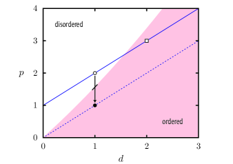
Figure 1: A slice in the space of RVB wavefunctions spanned by the lattice dimension $d$ and the powerlaw exponent $p$ of the long-bond tail. Spin models with local, nonfrustrating interactions live along the line $p=d+1$. Those with long range, nonfrustrating interactions live in the band $d\leq p\leq d+1$. The nearest neighbour Heisenberg model is indicated with an open circle ($d=1$) and an open square ($d=2$). In one dimension, the path from $p=2$ to $p=1$ (from open circle to filled circle) passes through a magnetic transition.

With the introduction of sufficiently long-range interactions (powerlaw decay with exponent $\alpha<3$), the decay exponent of the bond amplitude function can be tuned continuously in the range $1<p<2$. See Fig. 1. For the linear spin chain (in a model related to Eq. (1) with $\lambda=1$), the critical $p_{\text{c}}$ is achieved at $\alpha_{\text{c}}=2.18(5)$. This compares favourably to the critical value $\alpha_{\text{c}}^{\text{qmc}}=2.225(25)$ determined by quantum Monte Carlo in Ref. Laflorencie05, and represents a significant improvement over the values predicted by spin wave theory, $\alpha_{\text{c}}^{\text{sw}}=2.46$, Laflorencie05 and by a numerical renormalization group method, $\alpha_{\text{c}}^{\text{rg}}=1.85$. Rabin80

RVB analysis—The singlet ground state of an even number of $S=\tfrac{1}{2}$ spins can be expressed in an overcomplete basis of bipartite VB states. Beach06 A simple RVB wavefunction can be constructed by assigning to each bond of odd length $r$ an amplitude $h(r)$ and taking as the total weight for each VB configuration the product of the amplitudes of the individual bonds:

$$\lvert h\rangle=\sum_{v}\biggl{[}\prod h(r)\biggr{]}\lvert v\rangle.$$ (2)

The sum in Eq. (2) is over all possible pairings of spins in opposite sublattices, and the product is over all bond lengths $r$ appearing in the VB configuration.

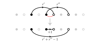
Figure 2: A valence bond is a singlet constructed from two spins in opposite sublattices and characterized by the directed distance between them. In a valence bond state, all the spins are paired to form valence bonds in one of the $(L/2)!$ possible configurations. The reconfiguration induced by the nearest-neighbour Heisenberg interaction is sketched above. The dotted (red) line shows where the interaction is applied. Bonds $r^{\prime},r^{\prime\prime}$ are mapped to $1,r^{\prime}+r^{\prime\prime}-1$.

The proper choice of $h(r)$ is determined by the model at hand. We observe that the application of a bipartite Heisenberg interaction to a VB state results in the reconfiguation of bonds depicted in Fig. 2. When acting between sites $i$ and $j$ (in opposite sublattices), separated by a distance $a=r_{ij}$, the interaction transforms bonds of length $r^{\prime}$ and $r^{\prime\prime}$ into bonds of length $a$ and $r=r^{\prime}+r^{\prime\prime}-a$. The steady-state solution Beach07b of this reconfiguration process is

$$h(r)=\int_{-\pi/2}^{\pi/2}\!\frac{dq}{\pi}\,e^{{\mathrm{i}}qr}h_{q},\ \ \ h_{q}=\frac{1-(1-J_{q}^{2})^{1/2}}{J_{q}},$$ (3)

where $J_{q}$ is the Fourier transform of the interaction normalized to $J_{q=0}=1$. In a model with NN interactions only, $J_{q}=\cos q$, and the long distance behaviour is

$$h(r)=\frac{2}{\pi(1+r^{2})}.$$ (4)

Numerical evaluation of Eq. (2) can be performed stochastically on lattices of finite size, as described in Ref. Beach07b, . We find that the RVB state for the Heisenberg chain (characterized by Eq. (3) with $J_{q}=\cos q$) has a magnetically disordered ground state and an $L\to\infty$ extrapolated energy $E=-0.4360(1)$, within 1.7% of the exact result $E=\log 2-1/4=-0.44315$. The discrepancy is somewhat large, but not unreasonably so given that our wavefunction was not variationally determined. Moreover, the RVB state performs worst in the disordered phase; the agreement is increasingly good the deeper we go into the magnetic region.

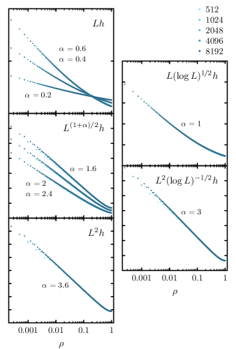
Figure 3: These log-log plots illustrate the five different scaling behaviours described in Eq. (10). Various renormalizations of the bond amplitude $h$ are plotted with respect to the reduced coordinate $\rho=2r/L$. All the vertical axes (labels suppressed) should be understood to start at $10^{0}$ and increase by one decade per tic ($10^{1}$, $10^{2}$, etc.).

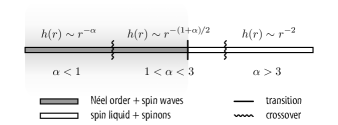
Figure 4: The long-bond behaviour of the amplitude function is powerlaw irrespective of the range of interaction, but the decay exponent changes as a function of $\alpha$. We identify three regimes. When $\alpha>3$, the bond amplitudes share the $h(r)\sim r^{-2}$ and $\omega_{q}\sim q$ behaviour of the nearest-neighbour Heisenberg model, differing only in the amplitudes of the short bonds and the value of the spinon velocity. In the intermediate regime $1<\alpha<3$, the decay exponent varies continuously, and the spin waves exhibit sublinear dispersion, $\omega_{q}\sim q^{(\alpha-1)/2}$. Below a critical ($\lambda$-dependent) $\alpha_{\text{c}}$, the spins develop long-range antiferromagnetic order. When $\alpha<1$, the interaction is superextensive and the system is close to being classically Néel ordered.

We now consider the long-range exchange integral

$$J_{ij}\sim\frac{1-(-1)^{i+j}}{\lvert r_{ij}\rvert^{\alpha}},$$ (5)

which is equivalent to the $\lambda=1$ case in Eq. (1), except that we have removed the interactions between spins in the same sublattice and compensated with coupling strength of opposite sign at neighbouring sites. This change has no real significance but it does simplify our analysis since nonbipartite interactions would require introducing a second update rule (different from the one shown in Fig. 2).

In this case, the $J_{q}$ to appear in Eq. (3) is

$$J_{q}=1+\frac{\sum_{n}[\cos(nq)-1]n^{-\alpha}}{\sum_{n}n^{-\alpha}}=1-\tfrac{1}{2}\xi^{2}_{\alpha}q^{2}+\cdots$$ (6)

Here, $n$ runs over all odd integers from $1$ to $L/2-1$, and, to leading order in $L$,

$$\xi_{\alpha}^{2}=\frac{\sum_{n}n^{2-\alpha}}{\sum_{n}n^{-\alpha}}=\begin{cases}\frac{1}{4}(\frac{1-\alpha}{3-\alpha})L^{2}&\alpha<1\\ \frac{L^{2}}{8\log L}&\alpha=1\\ \frac{L^{3-\alpha}}{(3-\alpha)2^{4-\alpha}(1-2^{-\alpha})\zeta(\alpha)}&1<\alpha<3\\ \frac{4\log L}{7\zeta(3)}&\alpha=3\\ \frac{(1-2^{2-\alpha})\zeta(\alpha-2)}{(1-2^{-\alpha})\zeta(\alpha)}&\alpha>3\end{cases}$$ (7)

When $\alpha>3$, $\xi_{\alpha}$ is O(1), and the long wavelength behaviour of $h_{q}=e^{-\xi_{\alpha}q}+O(\xi_{\alpha}^{3}q^{3})$ is integrable; hence,

$$h(r)=\frac{2\xi_{\alpha}}{\pi(\xi_{\alpha}^{2}+r^{2})}.$$ (8)

This is the same form we found for $J_{q}=\cos q$, except that $\xi_{\alpha}$, which controls the length scale at which the $r^{-2}$ tail is cut off, is now $\alpha$ dependent. In the limit $\alpha\to\infty$, $\xi_{\alpha}\to 1$, and we recover Eq. (4).

As $\alpha\to 3^{+}$, $\xi_{\alpha}$ diverges, and $h(r)$ changes functional form to $r^{-2}(\log r)^{1/2}$ at $\alpha=3$. There is an additional crossover at $\alpha=1$, where $h(r)$ goes as $r^{-1}(\log r)^{-1/2}$. Otherwise, the bond amplitude has a continuously variable decay exponent: $r^{-\alpha}$ for $\alpha<1$, and $r^{-(1+\alpha)/2}$ for $1<\alpha<3$. These results can be demonstrated by noting that $h(r)$ obeys the relation

$$h(r)=\frac{\xi_{\alpha}}{L^{2}}H_{\alpha}\biggl{(}\frac{2r}{L}\biggr{)}$$ (9)

with a scaling function

$$H_{\alpha}(\rho)\sim\begin{cases}\rho^{-\alpha}&\alpha<1\\ \rho^{-1}(\log\rho)^{-1/2}&\alpha=1\\ \rho^{-(\alpha+1)/2}&1<\alpha<3\\ \rho^{-2}(\log\rho)^{1/2}&\alpha=3\\ \rho^{-2}&\alpha>3\end{cases}$$ (10)

as verified by data collapse in Fig. 3.

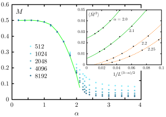
Figure 5: $\langle\hat{M}^{2}\rangle=(1/L^{2})\sum_{ij}(-1)^{i+j}\langle\mathbf{S}_{i}\cdot\mathbf{S}_{j}\rangle$, the staggered structure factor, is computed for lattices up $L=8192$ in size. The main plot shows the magnitude of the staggered magnetic moment, $M=\langle\hat{M}^{2}\rangle^{1/2}$, as a function of $\alpha$. The value of $M$ in the thermodynamic limit is marked with a solid (green) line. The inset shows the finite-size scaling of $\langle\hat{M}^{2}\rangle$ in the vicinity of the magnetic quantum critical point. The extrapolations to $1/L=0$ are draw with solid (green) or dashed (orange) lines depending on whether the intersection with the y-axis is positive. We estimate that the critical point lies in the range $2.1<\alpha_{\text{c}}<2.2$.

From what we know about the RVB ground state, it is possible to make a reasonable guess for the excitation spectrum $\omega_{q}$. Wherever the system is Néel ordered, the low-lying excitations are magnons. These spin-1 excitations can be created by promoting in succession each singlet bond in the RVB state to a triplet (along with the appropriate $q$-dependent phase factor): at the mean field level, one finds that $h_{q}\sim e^{-\omega_{q}}$ in the $q\to 0$ limit. Beach07a With this identification, $\omega_{q}\sim q$ when $\alpha>3$, and $\omega_{q}\sim q^{(\alpha-1)/2}$ when $1<\alpha<3$.

Numerical evaluation of the RVB wavefunction over a range of $\alpha$ reveals the phase diagram summarized in Fig. 4. We find that the staggered moment, shown in Fig. 5, is nearly saturated at $M=0.5$ throughout the $\alpha<1$ semi-classical region. $M$ decreases monotonically across the intermediate regime $1<\alpha<2$ and vanishes continuously at some $\alpha=\alpha_{\text{c}}$. Quantum disorder for $\alpha>3$ is guaranteed by theorem. Parreira97

Under the assumption of $\omega_{q}\sim q^{(\alpha-1)/2}$ spin excitations, the staggered structure factor exhibits $1/L^{(3-\alpha)/2}$ scaling. Laflorencie05 Accordingly, the inset in Fig. 5 shows it vanishing somewhere in the range $2.1<\alpha_{\text{c}}<2.2$. A more sophisticated finite-size scaling analysis (see Fig. 6), based on data collapse of the Binder cumulant, Binder81 indicates $\alpha_{\text{c}}=2.18(5)$. The correlation length exponent extracted from the fit, $\nu=2.4(2)$, is in agreement with the large-$N$ prediction of the corresponding $N$-component vector theory: Laflorencie05 namely, $\nu=1/(\alpha_{\text{c}}-1)$ for $1<\alpha_{\text{c}}\leq 5/3$, and $\nu=2/(3-\alpha_{\text{c}})$ for $5/3\leq\alpha_{\text{c}}<3$.

The transition is in the quantum percolation class. Vojta05 As the range of interaction is ramped up, the bonds in the RVB state grow longer, and the overlap loops increase in size. Across the magnetic transition, the scaling dimension $D$ of the average loop size ($\sim L^{D}$) changes discontinuously from $D=0$ to $D=1$. At criticality, the loops have fractal dimension $0<D_{f}<1$, and the dynamical exponent is fixed by $z=D_{f}$. This explains the observation in Ref. Laflorencie05, that $z<1$. (Analogous behaviour Beach07a is found in two dimensions for radially symmetric bond amplitude functions.)

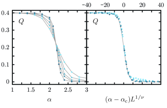
Figure 6: (Left) $Q=1-\langle\hat{M}_{z}^{4}\rangle/3\langle\hat{M}_{z}^{2}\rangle^{2}$, the Binder cumulant, is plotted as a function of $\alpha$ for lattices of increasing size. (The curves have increasing slope, approaching a step function for $L\to\infty$). The data points are shaded as in Figs. 3 and 5. The lines, connecting points of equal $L$, emphasize the invariance of $Q$ at $\alpha=\alpha_{\text{c}}$. (Right) The same data are replotted with an $\alpha_{\text{c}}$ shift and $L^{1/\nu}$ rescaling of the horizontal axis. Good data collapse is acheived for $\alpha_{\text{c}}=2.18$ and $\nu=2/(3-\alpha_{\text{c}})=2.44$. The line $(1/5)[1-\tanh(x/5)]$ is drawn as a guide to the eye.

Conclusions—The NN Heisenberg chain has a quantum disordered ground state, but the addition of long-range, antiferromagnetic interactions can drive the formation of magnetic LRO. The ground state wavefunction evolves smoothly across the phase boundary. Its structure on both sides of the transition is essentially that of a factorizable RVB wavefunction whose bond amplitudes decay as a powerlaw in the bond length. Only the value of the decay exponent changes across the transition.

The onset of Néel order can be understood as a quantum percolation transition in which the VB loops become system-spanning. The dynamical exponent $0<z<1$ is equal to the fractal dimension of the VB loops that are formed at criticality. The exact point at which the transition occurs and the value of the critical exponents there depend sensitively on the bond distribution.

The RVB picture is often invoked in a loose, heuristic way. Here, we have presented a concrete RVB wavefunction that proves to be a practical computational tool. Many aspects of the unbiased quantum Monte Carlo results can be reproduced by the RVB wavefunction with dramatically less computational effort.

The author acknowledges helpful discussions with Nicolas Laflorencie. This work was supported by the Alexander von Humboldt Foundation.

References

- (1) F. Haldane, Phys. Rev. B 25, 4925 (1982).
- (2) I. Affleck, D. Gepner, H. J. Schultz, and T. Ziman, J. Phys. A 22, 511 (1989); T. Giamarchi and H. J. Shulz, Phys. Rev. B 39, 4620 (1989); R. R. P. Singh, M. E. Fisher, and R. Shankar, Phys. Rev. B 39, 2562 (1989).
- (3) A. W. Sandvik, Phys. Rev. B 56, 11678 (1997); B. B. Beard and U.-J. Wiese, Phys. Rev. Lett. 77, 5130 (1996); H.-P. Ying and U.-J. Wiese, Z. Phys. B 93, 147 (1994).
- (4) E. V. Castro, N. M. R. Peres, K. S. D. Beach, and A. W. Sandvik, Phys. Rev. B 73, 054422 (2006); J. D. Reger, J. A. Riera, and A. P. Young, J. Phys.: Condens. Matter 1, 1855 (1989).
- (5) P. Bruno, Phys. Rev. Lett. 87, 137203 (2001); N. D. Mermin and H. Wagner, Phys. Rev. Lett. 17, 1133 (1966).
- (6) N. Laflorencie, I. Affleck, and M. Berciu, J. Stat. Mech. P12001 (2005).
- (7) J. M. Rabin, Phys. Rev. B 22, 2420 (1980).
- (8) E. Yusuf, A. Joshi and K. Yang, Phys. Rev. B 69, 144412 (2004).
- (9) G. Rumer, Gottingen Nachr. Tech. 1932, 377 (1932); L. Pauling, J. Chem. Phys. 1, 280 (1933); L. Hulthén, Arkiv Mat. Astron. Fysik 26A, No. 11 (1938).
- (10) K. S. D. Beach, arXiv:0709.3297v1 (unpublished).
- (11) K. S. S. Beach, arXiv:0707.0297v1 (unpublished).
- (12) S. Liang, B. Doucot, and P. W. Anderson, Phys. Rev. Lett. 61, 365 (1988).
- (13) K. S. D. Beach and A. W. Sandvik, Nucl. Phys. B 750, 142 (2006).
- (14) M. Havilio abd A. Auerbach, Phys. Rev. Lett. 83, 4848 (1999); ibid., Phys. Rev. B 62, 324 (2000).
- (15) J. R. Parreira, O. Bolina and J. F. Perez, J. Phys. A 30, 1095 (1997).
- (16) K. Binder, Z. Phys. B 43, 119 (1981).
- (17) T. Vojta and J. Schmalian, Phys. Rev. Lett. 95, 237206 (2005).