Chandra ACIS Survey of M 33 (ChASeM33): A First Look

Abstract

We present an overview of the Chandra ACIS Survey of M 33 (ChASeM33): A Deep Survey of the Nearest Face-on Spiral Galaxy. The 1.4 Ms survey covers the galaxy out to $R\approx 18\arcmin\/(\approx 4$ kpc). These data provide the most intensive, high spatial resolution assessment of the X-ray source populations available for the confused inner regions of M 33. Mosaic images of the ChASeM33 observations show several hundred individual X-ray sources as well as soft diffuse emission from the hot interstellar medium. Bright, extended emission surrounds the nucleus and is also seen from the giant H ii regions NGC 604 and IC 131. Fainter extended emission and numerous individual sources appear to trace the inner spiral structure. The initial source catalog, arising from $\sim$ $2/3$ of the expected survey data, includes 394 sources significant at the $3\sigma$ confidence level or greater, down to a limiting luminosity (absorbed) of $\sim$1.6$\times 10^{35}$ erg s^-1 (0.35 – 8.0 keV). The hardness ratios of the sources separate those with soft, thermal spectra such as supernova remnants from those with hard, non-thermal spectra such as X-ray binaries and background active galactic nuclei. Emission extended beyond the Chandra point spread function is evident in 23 of the 394 sources. Cross-correlation of the ChASeM33 sources against previous catalogs of X-ray sources in M 33 results in matches for the vast majority of the brighter sources and shows 28 ChASeM33 sources within 10″ of supernova remnants identified by prior optical and radio searches. This brings the total number of such associations to 31 out of 100 known supernova remnants in M 33.

1. Introduction

M 33 is a late-type Sc spiral galaxy located at a distance of 817$\pm$58 kpc (Freedman et al., 2001) and is the third largest spiral in the Local Group after M 31 and the Milky Way. The galaxy’s intermediate inclination angle of 56°$\pm$1° (Zaritsky et al., 1989), low foreground absorption (galactic $\mbox{$N_{\rm H}$}\sim 6.0\times 10^{20}$ cm^-2, Dickey & Lockman, 1990; Stark et al., 1992), and modest internal extinction make it the ideal target for exploring the global structure of the interstellar medium (ISM) and the stellar populations that shape it.

M 33 has been the subject of numerous previous X-ray studies, beginning with the Einstein Observatory (Long et al., 1981; Markert & Rallis, 1983; Trinchieri et al., 1988), which discovered 17 sources (including one that is probably a foreground star and one a background active galactic nuclei (AGN)). The most dominant source by far is associated with the nucleus, with $L_{X}\sim 1$$\times 10^{39}$ erg s^-1, making it the brightest persistent source in the Local Group. In addition to these individual sources, substantial unresolved emission was detected. ROSAT observations by Schulman & Bregman (1995) and Long et al. (1996) expanded the list of individual X-ray sources to 57 and showed that diffuse emission may trace the spiral arms near the nucleus. Through retrospective combination of all the ROSAT observations, Haberl & Pietsch (2001) found 184 X-ray sources within 50′ of the nucleus, a larger radius than in previous studies and including a number of foreground and background objects.

Most recently, Pietsch et al. (2004) and Misanovic et al. (2006) reported 447 individual X-ray sources in a deep XMM-Newton survey of M 33 within the $D_{25}$ optical elliptical isophote (semi-major axis $\sim 32\arcmin\/$). They characterized some of these sources based on X-ray hardness ratios and identified several dozen of these with supernova remnants, X-ray binaries and supersoft sources in M 33  based on cross-correlations with optical, radio, and infrared catalogs. In addition, they identified a number of foreground stars and background galaxies. Two of the transient sources were identified with optical novae in M 33 (Pietsch et al., 2005) and other transients were identified as probable X-ray binaries (Misanovic et al., 2006). Grimm et al. (2005) constructed a source list containing 261 sources and a luminosity function from Chandra observations that covered a $0.16~{}{\rm deg^{2}}$ region including the center of the galaxy and a region to the northwest of the center.

It is apparent in X-ray maps from XMM-Newton and earlier missions that M 33 is very confused in its inner regions where the density of individual sources becomes highest and the truly diffuse emission is strongest. We therefore proposed to use Chandra’s superior angular resolution with the Advanced CCD Imaging Spectrometer (ACIS, Garmire et al., 2003) to conduct the Chandra ACIS Survey of M33 (ChASeM33). We are obtaining deep, high-resolution images of the inner regions of M 33  out to a radius of $\approx 18\arcmin\/$ or $\approx 4$ kpc (1″$\sim$ 4 pc). A total of 1.4 Ms of Chandra observations are devoted to this project, divided among seven ACIS fields. Each field is observed for a total of 200 ks divided between two (or more) visits separated by 5–12 months. The first observation of the survey was executed in September 2005. In this paper, we report on the first group of these observations in which each field was observed at least once. This first group of observations allows us to create mosaic images of the region covered by the survey and to produce an initial source catalog, at typically half the depth of the complete survey. The primary objectives of the ChASeM33 are to: (1) establish the morphology of extended sources such as SNRs and superbubbles, (2) locate the optical counterparts – globular clusters, stars, and background AGN – of a large fraction of the point sources, and (3) study the association of various sources with the Population I and II components of M 33. In addition, ChASeM33 will provide long-duration observations for variability studies and transient detection. Given that much work can be pursued on these objectives with the partial survey data, we present here an overview paper that describes the survey and its advantages over previous surveys, discusses analysis techniques, and presents an intermediate source list with basic source characterization.

Some individual results from the ChASeM33 survey have already been published. Early observations of a field containing the eclipsing X-ray binary (XRB) M 33 X-7 resolved the eclipse ingress and egress for the first time and indicated that M 33 X-7 is the first known eclipsing black hole X-ray binary (Pietsch et al., 2006a). Furthermore, we found the eclipse and orbital period of the XMM-Newton source #47 from Pietsch et al. (2004, hereafter PMH04) in the ChASeM33 observations (Pietsch et al., 2006b). The likely optical counterpart also shows variability; therefore, this source is the second high-mass X-ray binary detected in M 33. Finally, the ChASeM33 data for the brightest X-ray SNR in M 33 (source #21 from the SNR catalog of Gordon et al., 1998, hereafter GKL98) are able to resolve the SNR from the giant H ii region NGC 592. Detailed spatial and spectral analysis of X-ray and other data shows a complex multiwavelength morphology indicating a shell expanding into an inhomogeneous medium, typical of an active star-forming region and suggesting that the SNR is indeed embedded within the H ii region (Gaetz et al., 2007).

The organization of this paper is as follows. In § 2 we describe the observations in detail (§ 2.1), the initial processing of the data (§ 2.2) , the creation of the mosaic images (§ 2.3), and the creation of the source catalog (§ 2.4). In § 3, we describe the characterization of the sources based on hardness ratios (§ 3.1), the identifications of the sources based on other catalogs (§ 3.2), the bright H ii region NGC 604 (§ 3.3.1), and the complicated southern arm region (§ 3.3.2). Finally, in § 4, we summarize the results of the paper.

2. Observations and Data Reduction

2.1. Observations

The ChASeM33 survey is designed to cover the central region of M 33 at a resolution $\lesssim 5\arcsec\/$ in order to resolve the source confusion in the inner galaxy found in earlier surveys, and to increase the number of known associations between X-ray sources and objects identified at other wavelengths. We chose seven overlapping ACIS-I fields, arranged such that all regions within a galactocentric radius of $\sim 4$ kpc lie no farther than 8′ off-axis in one or more fields (at 8′ off-axis, the 50% (90%) encircled-energy radius at 1.5 keV of the Chandra PSF is 3″ (7″)). Figure 1 shows the positions of the ChASeM33 fields on a deep ${\rm H}\alpha$ image taken from the 0.6m Burrell Schmidt telescope on Kitt Peak (McNeil & Winkler, 2006). We chose the ACIS-I array for the survey because of its larger field of view (FOV) at small off-axis angles compared to the ACIS-S array. The circles drawn in Figure 1 are contained inside the square $17\arcmin\times 17\arcmin$ FOVs of the ACIS-I array and indicate the regions within 8′ of the on-axis point.

Our program was designed to comprise two long ($\sim 100$ ks each) uninterrupted observations of each field, separated by six months or more, although in some cases, scheduling constraints dictated a larger number of shorter observations. ChASeM33 observations began in September 2005; in this paper we present the observations performed in the first year of observations (i.e., through August 2006). The observations are summarized in Table 1. At this point each field had been observed for roughly half of the 200 ks total time, and two fields (4 and 6) have their observations complete. In addition to the ChASeM33 observations, we utilized two archival ACIS-I observations of M 33 (OBSIDs 1730 & 2023), one centered on the nucleus and one centered on the bright H ii region NGC 604. There are two other archival observations of M 33 which we chose not to use since one (OBSID 786) was conducted with the ACIS-S array with its smaller FOV and the other (OBSID 787) was conducted in subarray mode with the ACIS-S array with an even smaller FOV. Some of the fields (1,2,3, second half of 4, and 7) were executed in continuous $\sim 100$ ks intervals. However some of the fields were broken into several pieces with field 6 being the most extreme example (6 observations, with one as short as 12 ks). To show the coverage, we display the exposure map of the ChASeM33 observations combined with the archival ACIS-I observations 1730 and 2023 in Figure 2. The combined exposure map is complicated, with the minimum exposure being $\sim 3.7\times 10^{6}~{}{\rm s~{}cm^{2}}$ and the maximum exposure $\sim 1.56\times 10^{8}~{}{\rm s~{}cm^{2}}$. The pattern of overlapping exposures results in a non-uniform exposure map, with the lowest exposures in the gaps between the CCDs and the highest exposure in the regions where 3 of the fields overlap. Chandra dithers while conducting observations, so that regions in the chip gaps receive some exposure (the lowest exposure typically being half that of the immediately surrounding regions unaffected by the dithered chip gap). Further complicating the exposure map is the fact that the overlapping regions typically combine data from different off-axis angles for which the response of the telescope is significantly different. Both the effective area and the angular resolution of the telescope decrease with increasing off-axis angle making it undesirable to simply add the data from overlapping observations. The implications of these effects for source detection and characterization are discussed in § 2.4.

2.2. Data Processing

All ChASeM33 observations are performed with ACIS-I as the primary instrument in ‘Very Faint’ (VFAINT) mode. The data are reprocessed with CIAO version 3.2.2 and CALDB version 3.1.0. First, we filter on the background flags for the VFAINT mode to improve the background rejection efficiency. We then apply the charge transfer inefficiency (CTI) correction to the archival observations (this correction was already applied to the ChASeM33 data in the standard processing) and the time-dependent gain correction appropriate for the time interval during which the data were acquired. The events file is then screened with grade and status filters, good time intervals are selected, and pixel randomization is removed. Finally, we check for background flares by creating a background light curve from the events on the ACIS-I3 chip, after removing point sources. We perform an iterative sigma-clipping algorithm to remove time intervals with count rates more than $3\sigma$ from the mean of each iteration, until all count rates are less than $3\sigma$ above the mean. Table 1 lists the effective exposure times after the light curves have been filtered. This filtering resulted in the selection of events which were used for the analysis discussed in this paper.

2.3. Mosaic Images

We created a mosaic image of the observations listed in Table 1, including the two archival pointings to increase the exposure and provide additional coverage. We selected events with off-axis angles $\leq 8.0\arcmin\/$ to include only the highest angular resolution data in these images and with energies $0.35<{\rm E}<8.0$ keV in order to maximize the X-ray signal compared to the background. The data were binned into $2\arcsec\/\times 2\arcsec\/$ pixels (a binning of $4\times 4$ on the original 0$\farcs$492 sky pixels). The exposure maps are computed using the CIAO tools mkinstmap and mkexpmap. For the instrument maps, we compute the spectral weights assuming a power-law spectrum with $\Gamma$ = 1.9 and $N_{\rm H}$= $1.0\times 10^{21}$ cm^-2. We adopt an $N_{\rm H}$ of $1.0\times 10^{21}$ cm^-2 based on the estimates of the Galactic column density of $5.7\times 10^{20}$ cm^-2 (Dickey & Lockman, 1990) and $6.3\times 10^{20}$ cm^-2 (Stark et al., 1992) and the total line-of-sight column density through M 33 which averages about $1.0\times 10^{21}$ cm^-2 (Newton, 1980). We adopt a power-law model with $\Gamma$ = 1.9 as representative of the intrinsic spectrum of AGNs (Pounds et al., 1994). The image is exposure-corrected and smoothed with a Gaussian filter with a $\sigma=3$ bins corresponding to 6″. Figure 3 shows this mosaic image for the energy band 0.35 – 8.0 keV. The nucleus dominates the center of the image at $\sim$ RA(J2000) = 01^h 33^m 50$\fs$9 , Dec(J2000) = +30° 39′ 36$\farcs$8 (hereafter all coordinates are provided in epoch J2000). There are numerous bright X-ray sources visible in this image, notable among them is the XRB X-7 at RA = 01^h 33^m $34\fs 12$ , Dec = +30° 32′ 11$\farcs$6. The diffuse emission is not as evident in this image as in the XMM-Newton data (Pietsch et al., 2004) due to the ACIS-I array’s lower sensitivity to soft X-rays. However, several bright diffuse objects are easily visible; e.g., NGC 604, the brightest H ii region in M 33, northeast of the nucleus at $\sim$ RA = 01^h 34^m 34^s , Dec = +30° 47′, and the H ii region IC 131, northwest of the nucleus at $\sim$ RA = 01^h 33^m 15^s , Dec = +30° 45′.

We also created images in narrower energy bands (soft [0.35 – 1.1 keV], medium [1.1 – 2.6 keV], and hard [2.6 – 8.0 keV]) to distinguish between softer and harder emission. The three-color mosaic image of all the ACIS-I observations of M 33 is presented in Figure 4. The image shows different types of sources in different colors: e.g., most of the known SNRs appear red or orange, while hard sources like XRBs or background AGN are blue or white. The nucleus appears white in the image since it is bright in all three bands. The H ii region NGC 604 appears rather red while the H ii region IC 131 appears green, a clear indication that the spectrum of IC 131 is significantly different from that of NGC 604. The three-color image also shows faint and soft diffuse emission northwest of the nucleus as well as extending from southeast to south which traces the southern spiral arm of M 33.

2.4. Source Catalog

We searched for candidate sources using the CIAO tool wavdetect. Each ChASeM33 observation or group of observations conducted at the same pointing and roll angle was searched; we did not search the archival observations. For each ACIS-I chip, we binned to 0.492″ sky pixels and ran wavdetect for the band 0.35–8 keV. We used a significance threshold of $1.0\times 10^{-6}$ which corresponds to a false detection probability of about 1 source per CCD (Freeman et al., 2002). To reduce spurious source detections at the chip edges, we used an exposure map (evaluated at 1.5 keV) and required that the exposure be at least 10% of the peak value. In order to be sensitive to spatial scales up to $\sim$ 0.5′, we used a power-of-2 sequence of scales from 1 to 64 pixels. Only detections with a significance of $>3\sigma$ as determined by wavdetect were considered for further investigation. The signal-to-noise ratio computed by wavdetect is the net counts divided by the Gehrels (1986) estimate for background error $\sigma_{B}=1+\sqrt{C_{B}+0.5}$, where $C_{B}$ is the estimate of background counts in the source detection region. These detections were used as input source positions for the software package ACIS Extract (Broos et al., 2002).

ACIS Extract is a multi-purpose source characterization package which computes source and background count rates and fluxes in a group of user-specified energy bands, computes source significance, extracts spectra and generates appropriate response files, among other items (see Broos et al., 2002, for details). Of particular interest and advantage for our analysis is the fact that ACIS Extract produces an extraction region tailored to match the Chandra point spread function (PSF) at the position of the source in each observation. This capability is crucial for our analysis since we have multiple, overlapping FOVs in which a particular source may end up at a variety of off-axis and azimuthal positions. Each of these positions requires a different extraction region based on the PSF to optimize the source signal compared to the background, since the Chandra PSF is a function of both off-axis angle and azimuthal angle. The software produces a background region for each source that excludes the source extraction regions of nearby sources. ACIS Extract allows a visual inspection of each source in each exposure along with an outline of the PSF. These visual inspections allowed us to flag clearly extended sources in the catalog and to remove duplicate sources that were observed in more than one observation in overlapping sections of fields. We also identified observations in which the source extraction region was affected by the “transfer streak” of the readout of the ACIS CCDs. Typically a source was affected by the transfer streak in only one observation (or group of shorter observations conducted at the same pointing position and roll angle). We then excluded those observations from the source characterization while retaining the observations in which the source was unaffected by the transfer streak. The inspections also allowed us to adjust the source positions in cases where there were multiple detections and the wavdetect source position chosen did not match the centroid of the most nearly on-axis observation of the source.

The final judgment on the significance of a source was based upon the source and background counts calculated by ACIS Extract in the 0.35–8.0 keV band. The signal-to-noise ratio calculated by ACIS Extract uses the difference between the Gehrels (1986) estimate for the Poisson upper limits on the source and background counts and the net extracted counts; this generally results in a lower significance than wavdetect. In this manner, we used wavdetect as a candidate source detection tool and used ACIS Extract as a source characterization tool. Our approach is conservative in two respects. First, for the two fields in which the first and second epoch observations were available (fields 4 and 6), we did not add the data and conduct a source detection on the summed data. We plan to conduct such an analysis on the full survey data and we expect that fainter sources will be detected in such an analysis. Second, we filtered twice on the source significance, once on the output of wavdetect and a second time on the output of ACIS Extract. It is conceivable that there are sources which were less significant than $3\sigma$ in the wavdetect output which would have become more significant than $3\sigma$ in the ACIS Extract output after the source and background extraction regions had been adjusted. We decided to be conservative in this first catalog and will explore alternative source detection techniques in a future paper.

We estimated the extended-source positions using an iterative “$\sigma$-clipping” algorithm as described in Ghavamian et al. (2005). Based on an initial position estimate and clipping radius, the centroid of the events (0.35–2.6 keV) within the clipping radius is evaluated. Events more than $n\sigma$ ($n=1.5-2$) from the centroid are removed, and a new centroid is evaluated. The procedure is repeated until convergence within 0.01 pixels is attained, or for a maximum of 10 iterations. For each extended source, this procedure was applied for selected observations in which the source was closest to on-axis, or contained the largest number of counts. We examined the exposure maps, and only included those observations for which the exposure was fairly uniform across the centroiding region (avoiding observations with the source near a chip edge). In many cases, more than one observation qualified, in which case we estimate a weighted mean position, where we weight by the net exposure time at that location on the CCD for the observation.

Finally, the ACIS Extract value of the source significance was applied to remove source candidates with less than $3\sigma$ detections in the 0.35-8.0 keV band, therefore forcing all of the objects in our final catalog to show $3\sigma$ significance by both measuring techniques. We measured all of the fluxes, spectra, and timing for our final source list using ACIS Extract. The ACIS Extract measurements include short-term and long-term variability information as well as fluxes. A variability study of the sources is in progress and will be addressed in future publications (Williams et al. 2007, private communication).

Table 2 is the source catalog of the ChASeM33 data containing 394 sources. The columns in Table 2 contain the source number, the position in RA(J2000) and Dec(J2000), the error in the position, the net counts after background subtraction, the count rate in the 0.35–8.0 keV band with the error in the count rate listed in parentheses, the photon flux (absorbed) in the 0.35–8.0 keV band with the error in the flux listed in parentheses, and the hardness ratios HR1 and HR2 as defined in § 3.1 with the appropriate errors listed in parentheses after each HR value. Extended sources are indicated by a superscript e on the source number; 23 sources show evidence of spatial extent beyond the local PSF. Given the source selection criteria described above, we estimate that the faintest source we could detect in a 100 ks observation, close to on-axis would have $\sim 15$ net counts. Source #385 is the source with the lowest number of net counts in our list with 16.4 net counts. The minimum number of counts necessary for a $3\sigma$ detection grows with off-axis angle as the PSF increases. We estimate that a source 8′ off-axis would need $\sim 30$ net counts to satisfy our source detection criteria. The photon fluxes were calculated in the three bands 0.35-1.1 keV, 1.1-2.6 keV, and 2.6-8.0 keV, using the net counts in the band, a mean effective area for that band, and the exposure time. The mean effective area for a band was computed assuming a flat spectrum, this partially accounts for the fact that the Chandra effective area is a strong function of energy. The photon fluxes in the individual bands were then summed to produce the photon flux in the 0.35-8.0 keV band. Therefore, we have not made any assumptions about the spectra of the sources to convert the detected counts into a photon flux, other than the assumption of a flat spectrum for the mean effective area. For illustrative purposes, we will now assume a model spectrum for the lowest and highest flux sources in our list and perform spectral fits in XSPEC to quantify what the range of energy fluxes might be for these assumed spectral models. The lowest flux source in the list is source #315, with a photon flux (0.35–8.0 keV) of $2.50\times 10^{-7}$ photons cm^-2 s^-1 which corresponds to an energy flux (0.35–8.0 keV, absorbed) of $8.4\times 10^{-16}$ erg cm^-2 s^-1 assuming a power-law spectrum with a photon index of 1.9 and an $N_{\rm H}$ of $1.0\times 10^{21}~{}{\rm cm^{-2}}$. This flux implies a luminosity (absorbed) of $6.7\times 10^{34}$ erg s^-1 at the distance of M 33. Even with the low number of counts, the reduced $\chi^{2}$ of the fit improves significantly when the $N_{\rm H}$ is allowed to vary, dropping from 1.51 to 0.48 for an $N_{\rm H}$ of $9.1\times 10^{21}~{}{\rm cm^{-2}}$. The fit with this model implies a luminosity (absorbed) of $1.6\times 10^{35}$ erg s^-1, $2.4\times$ higher than the estimate with an $N_{\rm H}$ of $1.0\times 10^{21}~{}{\rm cm^{-2}}$. The highest flux source is of course the nucleus (#200 in this list) with a photon flux of (0.35–8.0 keV) of $1.95\times 10^{-3}$ photons cm^-2 s^-1. A spectral fit with an absorbed power-law model returns an $\mbox{$N_{\rm H}$}=4.5\times 10^{21}~{}{\rm cm^{-2}}$, an index of 1.99, an energy flux (0.35–8.0 keV, absorbed) of $5.1\times 10^{-12}$ erg cm^-2 s^-1, and a luminosity (absorbed) of $4.1\times 10^{38}$ erg s^-1. We note that this source is significantly piled-up and the measured flux and luminosity are underestimates of the true values. The analysis of the nucleus and other sources significantly affected by pileup will be discussed in a future paper.

3. Analysis and Discussion

The primary product of our analysis has been the creation of the source catalog shown in Table 2. We now make use of that catalog to begin to characterize the sources through their hardness ratios, and to identify some of the sources by cross-correlation with other catalogs. In addition to the results based on the source catalog, we present two examples of the types of analyses which this rich data set allows, namely preliminary results on the H ii region NGC 604 and the southern arm region.

3.1. Hardness Ratios

Using the background-subtracted photon fluxes for the ChASeM33 sources, we created a hardness ratio diagram (Fig. 5). We construct hardness ratios using a definition similar to that described in Prestwich et al. (2003) from background-subtracted fluxes for soft ($S$), medium ($M$), and hard ($H$) bands:

$$\mathrm{HR1}={(M-S)\over(S+M+H)},$$ (1)

and

$$\mathrm{HR2}={(H-M)\over(S+M+H)},$$ (2)

where in our case, $S=0.35$–1.1 keV, $M=1.1$–2.6 keV, and $H=2.6$–8 keV (the same bands used for the three-color image in §2.3). We estimate the uncertainties on the fluxes in a given band by taking the differences between the Gehrels (1986) upper limits and the net counts for the band. The uncertainties for the hardness ratios are then estimated by propagating the flux errors assuming Gaussian statistics (the uncertainties are included in parentheses behind the HR value in Table 2).

The hardness ratio HR2 is plotted against HR1 in Fig. 5. We indicate the limiting fluxes by solid black lines: $S=0$ (upper left to right center), $M=0$ (right center to bottom center), and $H=0$ (bottom center to upper left). We plot all the sources, including those listed with zero or negative fluxes in some bands. Most of the latter lie near the boundary of the allowed region, and are clearly real sources with spectra similar to those just within the allowed region. If the true flux in a band were zero, the uncertainties associated with background subtraction would yield a negative observed flux roughly half the time. We note that Hong et al. (2004) and Park et al. (2006) have suggested that the “quantile” method and Bayesian approaches have significant advantages over the traditional hardness ratios method for faint sources which have a low number of counts in a given band. We will consider the use of these new methods in our final catalog paper. The source hardness ratios are plotted as symbols with sizes indicating the 0.35–8 keV photon fluxes (photons cm^-2 s^-1): $\leq 10^{-6}$ (smallest symbols), $10^{-6}$–$10^{-5}$, $10^{-5}$–$10^{-4}$, $10^{-4}$–$10^{-3}$, and $>10^{-3}$ (largest symbols). GKL98 objects (discussed below) are plotted with red symbols, extended objects which are not in the GKL98 list are plotted as cyan, and the rest are plotted in blue. In each case, apparently nonextended sources are plotted as circles, and extended sources are plotted as squares. For reference, we plot loci for absorbed powerlaws computed using XSPEC (again the HR values are based on the photon fluxes in § 2.4 which assume a flat spectrum to compute the mean effective area in the three bands). The black solid curve shows the locus for powerlaws with absorption $N_{\mathit{H}}=10^{21}\,\mathrm{cm}^{-2}$, and powerlaw index $\Gamma$ ranging from 0 to 3; the large black “$\times$” symbol indicates the $\Gamma=1.9$ powerlaw. The black dashed curve is similar except that a larger absorbing column, $N_{\mathit{H}}=3\times 10^{21}\,\mathrm{cm}^{-2}$, is assumed. The large black “$+$” symbol indicates the $\Gamma=1.9$ powerlaw for this case.

We expect the large clump of sources in the center of the diagram will prove to be a combination of XRBs in M33 and background AGN. The nucleus is indicated by the large blue circle near the center of the diagram. We also detected objects associated with the GKL98 list of optically-identified SNRs, and some clearly extended sources. The sources identified with GKL98 objects are plotted with red symbols, again using circles for nonextended sources (18 objects), and squares for extended sources (8 objects). Finally, in addition to the GKL98 extended objects, we detect an additional 5 objects which do not appear in the GKL98 list; these are plotted as blue squares. As expected, the GKL98 supernova remnants tend to cluster in the soft portion of the diagram (bottom center, near the $H=0$ line).

In order to explore the distribution of the ChASeM33 sources across the galaxy we have plotted the positions of the sources on a ${\rm H}\alpha$ image (McNeil & Winkler, 2006) in Figure 6. We have used the same symbols and colors as those used in the hardness ratio diagram in Figure 5. The concentration of SNRs along the southern spiral arm is evident in this image. Also interesting is the clump of unidentified sources (indicated by the medium-size blue circles) just south of the concentration of SNRs. This region warrants a closer examination in the future. The nucleus is again clearly indicated by the large blue circle in the center of the image. We note that at least half of the sources in the ChASeM33 catalog and this image are expected to be foreground and background sources. One would expect the foreground and background sources to be uniformly distributed across the region of the survey. Therefore, any concentration of sources aligned with structure in the galaxy, such as the southern spiral arm, is more likely to have a higher percentage of M 33 sources. Identifying which sources are related to M 33 and those which are unrelated is a non-trivial task which will require a significant effort to conduct optical followups of these sources. A careful study of the characteristics of the X-ray source population in M 33 will require such an identification and an accurate means of estimating the contribution of foreground and background sources.

3.2. Comparison with Previous Catalogs

In order to gain some perspective on the sources contained in this catalog of X-ray sources in M33, we have cross-correlated the ChASeM33 sources with sources detected in previous X-ray studies as well as with a number of catalogs constructed from optical and radio studies of M 33. A total of 17 sources were identified in the vicinity of M 33 using Einstein (Trinchieri et al., 1988). Of these, 13, including all of the brighter sources, lie within 2″ of ChASeM33 sources. The sources that were missed by us were either outside of the region that was surveyed in ChASeM33, were detected only with the Imaging Proportional Counter, or were detected at very low statistical significance in the Einstein data. Excluding for the moment other Chandra observations, the deepest X-ray surveys of M 33 are those carried out by PMH04 and Misanovic et al. (2006, hereafter MPH06) using XMM-Newton. MPH06 took the most care in using data from individual observations from which one could obtain accurate source positions and their catalog contains 350 sources with typical position errors of 2″ for the brighter sources. PMH04 included more data and their catalog has 408 sources, 97 of which are not contained in the source list compiled by MPH06. Of the sources in the PMH04 and MPH06 catalogs, 225 and 189 of the sources are found in regions covered by the ChASeM33 survey (at an effective exposure exceeding $\rm 10^{6}\rm\>s~{}cm^{-2}$ at 1 keV). The 3$\sigma$ position errors for the faintest sources in both XMM-Newton surveys are about 7″. Assuming this positional uncertainty, there are 198 and 154 ChASeM33 sources that have counterparts in the two surveys, indicating a high degree of overlap. The source correlations are listed in Table 3. Not surprisingly, given the higher resolution of Chandra, there are cases where multiple ChASeM33 sources are identified with a single XMM-Newton source. Of the XMM-Newton sources that are in the region we surveyed , there are 28 and 26 sources, respectively, that were not detected. A superficial inspection of the XMM-Newton sources that were not detected shows that they tend to be the fainter sources, with a median count rate 2.5 times lower than the XMM-Newton sources that have counterparts. They also tend to have softer X-ray spectra than the sources that have counterparts; for example, in the PMH04 list, the sources without counterparts have a mean (0.5-1 keV vs 1-2 keV) hardness ratio of -0.14, compared to +0.15 for the sources with counterparts, which may reflect XMM-Newton’s greater effective area at low energy compared with ACIS-I.

Grimm et al. (2005, hereafter GMZ05) created a source catalog from their analysis of 3 earlier Chandra observations of M33, two centered on the nucleus of M33, and one centered on the star-forming H ii region, NGC604. They report a total of 261 sources; based on a detection using wavdetect in any of the 3 observations and in any of 3 bands (soft: 0.3–2.0 keV, hard: 2.0–8.0 keV, and total: 0.3–8.0 keV), with positional uncertainties that are typically $<2$″, but are occasionally considerably larger (up to 10″). Of these 261 sources, only 145 have counterparts in the ChASeM33 source list allowing a position uncertainty of 3″, and 99 remain unidentified assuming a position uncertainty of 10″. This difference clearly demands explanation, especially since the ChASeM33 exposures are deeper than (and in some cases overlap with) those analyzed by GMZ05. Of the 261 sources identified by GMZ05, 249 are in regions where the effective exposure exceeds $\rm 10^{6}\rm\>s~{}cm^{2}$ at 1 keV, and so disjoint fields of view do not explain the difference. Instead, the principal reason for this difference is that GMZ05 used far less conservative source selection criteria than those we have used, detailed in section 2.4. While our source selection required detections of at least $3\sigma$ significance in both wavdetect and ACIS Extract, their selection criteria demanded only a detection by wavdetect at any significance. Of the 261 sources listed by GMZ05 there are 144 which have fluxes which are measured at $3\sigma$ in any one of the observations analyzed by GMZ05; of these 112 are matched assuming a position uncertainty of 3″, rising to 122 if a position uncertainty of 10″ is allowed. Some of the remaining differences are likely due to the time variability of the sources. If we restrict ourselves to the 29 sources with count rates determined at $10\sigma$ detected by GMZ05, there are still 4 which are unmatched assuming a position uncertainty of 10″; of these, two (J013435.1+305646 and J013444.6+305535 ) were not in regions included in the ChASeM33 data, one (J013433.7+304701) is located in NGC604 and we excluded it as a separate source, and the remaining source appears to be time-variable.

An important goal of the ChASeM33 survey is to study the X-ray properties of the SNR population in M33. The most extensive catalog of SNRs in M33 remains the catalog of GKL98, which contains 98 SNRs identified on the basis of strong [S II]:${\rm H}\alpha$ emission. Ghavamian et al. (2005) identified two more SNRs based on elevated [S II]:${\rm H}\alpha$ ratios and the soft X-ray spectra from XMM-Newton, bringing the total to 100. After updating the positions of a few of the SNRs based on our interference filter imagery, we find that 28 lie within 10″ of ChASeM33 source positions. Nearly all of these sources have very soft X-ray spectra, consistent with their identification as SNRs. With two exceptions, a comparison of X-ray surface brightness distribution and ${\rm H}\alpha$ images in the vicinity of each of these sources also supports their identification as SNRs. The exceptions are ChASeM33 source #222, which is close to GKL98-59, and ChASeM33 source #242, which is close to GKL-66. Both of these sources appear point-like, and lie outside the optical nebulosity associated with the SNR. Source #242 is also the only candidate SNR that has a hard X-ray spectrum. We (Ghavamian et al., 2005) had previously searched M33 for SNRs using Chandra archival data; in that search, 21 SNRs were found to match objects in the GKL98 list. Of these, 16 are contained in our list of SNRs with X-ray counterparts. However, there were 5 SNRs in our earlier list that were not confirmed here. This is almost surely due to the fact that, in the earlier search, we used band-passes that were optimized for SNRs rather than the broad-band used here. Thus, excluding the two doubtful associations discussed above, the total number of optically identified SNRs detected with Chandra now totals 31, roughly 1/3 of all of the SNRs that are known in M 33. PMH04 performed an initial search of the XMM-Newton data for SNRs using criteria similar to our own. They identified 21 of the GKL98 SNRs. In their reanalysis of the data, MPH06 confirmed 15 of these, and suggested that 3 others (corresponding to SNRs 21, 28, and 55) were not SNRs since they exhibited time variability. All of the latter are currently included in our list of identifications, though it is clear that further studies are warranted. In the Chandra data, SNR21 is resolved as an elliptical shell with a size of 5″; it was the subject of a detailed discussion (Gaetz et al., 2007).

The USNO3 catalog contains about 8600 “stars” in the region that was surveyed as part of ChASeM33, 69 of which lie within 3″ of ChASeM33 sources. The majority of these are not single stars, but instead represent a heterogeneous collection of objects, including stellar associations, H ii regions, and background galaxies. Given this number of objects and an allowed error of 3″, one expects about 24 chance coincidences. Therefore, although many of the correspondences likely represent a physical association, the effort to determine which are real and which are not is beyond the scope of this initial discussion of the ChASeM33 sources. Therefore in Table 3, we have identified only the 12 objects with an R magnitude of less than 15 that lie within 3″ of a ChASeM33 X-ray source; there are 436 USNO3 sources with an R magnitude of less than 15 and thus only one of these associations is expected to occur by chance. A number of these sources have already been identified as stars by PMH04 or MPH06, and Hatzidimitriou et al. (2006) had already studied the counterparts of 6 of these sources.

Using the Ultraviolet Imaging Telescope, Massey et al. (1996) identified 356 UV bright sources brighter than $2.5\times 10^{-15}\rm\>\>{\rm ergs\>cm^{-2}\>s^{-1}\>\AA^{-1}}$, located preferentially along the spiral arms, and nearly all of which (351) are in the region surveyed in ChASeM33. The objects in this list contain many O and early B-type supergiants, as well as a number of ”super luminous” Wolf-Rayet stars and OB associations. Ten of these sources are located within 5″ of ChASeM33 X-ray sources, of which only one is expected by chance, and these are listed in Table 3. This is an indication that the X-ray source population in M33 is associated strongly with star formation. We also compared the ChASeM33 source list to a variety of other catalogs, including the lists of star cluster candidates in M33 compiled by Sarajedina & Mancone (2007), of planetary nebulae in M33 by Ciardullo et al. (2004), of emission line objects by Calzetti et al. (1995), and of giant molecular clouds by Engargiola et al. (2003). Although there were a small number of coincidences, in nearly all cases the number of coincidences was close to that expected by chance. This does not imply that there are no physical associations with these objects in specific cases, but does imply that much more work will be required to isolate the subset of sources that have a physical association with these source populations. A more detailed analysis of such correlations will be considered when the full ChASeM33 dataset has been analyzed.

Besides position and hardness ratio information, time variability arguments can be used to strengthen identifications. An interesting source in this respect is ChASeM33 #175 ([PMH04] 196) only  1′ west southwest of the bright nuclear source X-8. Optical colors, as well as X-ray hardness ratio, and ${\rm f_{\mathit{x}}/~{}f_{\mathit{opt}}}$, suggested an identification with an M-type star in the foreground. This identification has been strengthened by X-ray flux variability detected in XMM-Newton observations (Misanovic et al., 2006). The optical spectrum allows the identification of the optical counterpart as a late M star with ${\rm H}\alpha$ emission indicating a flare star, and indeed X-ray flaring was detected in early Chandra ACIS observations of the source (Hatzidimitriou et al., 2006). ChASeM33 #175 was in the field of view of several ChASeM33 pointings which allowed us to search for flares in a much larger dataset. While in many observations little or no variability is present, a strong flare is detected in ObsID 6383 on 16 June 2006 with a FWHM of  2000s (Fig. 7). During the flare the source reaches a count rate of more than $7\times 10^{-2}$ cts s^-1 in the 0.5–2.5 keV band. In total  400 cts ( 150 during the flare) were collected from the source.

3.3. Resolving Confused Regions

Several regions in M 33 have extended X-ray emission confused with point sources and/or high source density. Attaining a better understanding of these regions was a prime motivation behind the ChASeM33 observations. Here we present our first analyses of two such regions: NGC 604 and the southern spiral arm.

3.3.1 The Giant H ii region NGC 604

An example of the power of the high-resolution images of M 33 from ChASeM33 is the complex X-ray structure within and around the giant H ii region NGC 604, as shown in Figure 8. The left image shows the Chandra ACIS-I image, binned into $2\arcsec\times 2\arcsec\/$ pixels, with the X-ray contours overlaid on the data. In the right panel we show a three-color image from archival HST WFPC2 observations (see Maíz-Apellániz et al., 2004), with the $I$ band in red (F814W, 200 s), ${\rm H}\alpha$ in green (F656N, 1000 s), and $V$ band in blue (F555W, 200 s), with the Chandra X-ray contours overlaid on the data. The Chandra image shows the hot diffuse gas inside the H ii region. There is bright X-ray emission from a point-like source inside NGC 604 (in projection), southeast of the bright cluster of stars. The Chandra image has also resolved a SNR (GKL98-94 and ChASeM33 source # 342) located south of the H ii region. The source to the east is probably a background source, as discussed below. This image demonstrates how essential the high angular resolution of Chandra is in separating the X-ray emission of the three discrete sources from the diffuse emission of NGC 604.

We perform spectral analysis of the prominent X-ray sources in this region using the ChASeM33 data. The diffuse emission in NGC 604 is well fit with a thermal emission model (APEC in XSPEC) with an absorbing foreground column density of $N_{\rm H}$ = (0.53$\pm$0.02) $\times 10^{21}$ cm^-2, a temperature corresponding to $kT=0.195\pm 0.007$ keV, and a flux (absorbed) of $F_{\mathrm{X}}$(0.5-2 keV) = $5.0\times 10^{-14}$ ergs cm^-2 s^-1; this does not include the bright point-like source inside NGC 604. The point-like source is located at RA = 01^h 34^m $32\fs 6$ , Dec = +30° 47′ 6″ and has a FWHM $\approx$ 1″. The photon statistics are too low to determine specific model parameters; its spectrum is consistent with its being a bright feature inside the overall diffuse emission.

The source at RA = 01^h 34^m $36\fs 4$, Dec = +30° 47′ 16″ with a FWHM = 1.08″, is most likely an AGN. For the spectrum, we get $N_{\rm H}$ = $(6.3\pm 0.9)\times 10^{22}$ cm^-2, with a photon index of $\Gamma=2.3\pm 0.4$. The flux (absorbed) $F_{\mathrm{X}}$(2-10 keV) = 3.2 $\times 10^{-14}$ ergs cm^-2 s^-1. This source is harder than the emission from NGC 604 and is nearly as bright as the diffuse emission. The significantly higher value of the $N_{\rm H}$ argues that this is a background AGN, likely with a significant amount of intrinsic absorption.

The SNR GKL98-94 is observed at RA = 01^h 34^m 33$\fs$0, Dec = +30° 46′ 40″, with an extent of 3.4$\pm$0.3″. This source is also faint with only $\sim$100 counts detected. It is well fit with a simple thermal model (APEC in XSPEC) with $N_{\rm H}$ = $0.56(+0.08,-0.18)\times 10^{22}$ cm^-2, $kT=0.25(+0.08,-0.02)$ keV, and $F_{\mathrm{X}}$(0.5-2 keV) = 2.5 $\times 10^{-15}$ ergs cm^-2 s^-1. According to these fits, both the SNR and the diffuse emission in NGC 604 show excess absorption compared to the Galactic column ($N_{\rm H}$ is roughly an order of magnitude higher than expected) which is likely due to significant amounts of dust and gas local to M 33, associated with the H ii region.

3.3.2 The Southern Spiral Arm Region

It is known that there are a large number of SNRs located in the southern spiral arm of M 33. Figure 9 shows a $9\farcm 3\times 15\farcm 6$ region around this spiral arm in different energy bands. In the first panel, we present the Chandra three-color image using the same bands in § 2.3, where the second panel shows the continuum-subtracted ${\rm H}\alpha$ image from the Local Group Galaxies Survey (LGGS, Massey et al., 2006), and the third panel is the Spitzer IRAC 3.6 $\mu$m image which is dominated by stars. The positions of the optical SNRs of the GKL98 list are marked by the circles labeled with the GKL98 catalog number. The images show that the optical SNRs are well-aligned with the southern spiral arm and that many of them show soft X-ray emission. There are 26 SNRs from the GKL98 catalog contained in this region, 10 of which have counterparts in the ChASeM33 source list (see Table 3 for details). Of the 16 SNRs without ChASeM33 counterparts, many show some evidence of subthreshold X-ray emission. GKL98 -46, -49, -67, -69, and -82 seem similar in that there is some X-ray emission near the position of the optical SNR, but the emission was too faint to satisfy the selection criteria for this version of our catalog. These types of sources may well become significant detections when all of the ChASeM33 data are combined. Several other sources are worthy of note in this image. GKL98-31 (ChASeM33 #123) is a bright X-ray source with a spectrum dominated by emission lines of O, Ne, and Mg. This SNR appears to be an analog of the X-ray O-rich SNR in the Small Magellanic Cloud 0103-72.6 (Park et al., 2003) and will be the subject of a forthcoming paper (Hughes et al. 2007, private communication). These data demonstrate the importance of Chandra’s high angular resolution for identifying the X-ray counterparts of the optical SNRs in such a crowded region and for cleanly separating the X-ray emission from one object from the surrounding objects for spectral analysis.

4. Summary

We have presented results from roughly the first half of the ChASeM33 survey of M 33, which covers the full area of the survey but at typically half the depth. Our total intensity image in the 0.35–8.0 keV band (Fig. 3) is dominated by the bright nucleus and surrounding diffuse emission, bright XRBs in M 33 (such as X-7), bright diffuse objects such as NGC 604 and IC 131, and bright background AGN and foreground stars. Our X-ray three-color image (Fig. 4) constructed from the three bands 0.35–1.1 keV, 1.1–2.6 keV, and 2.6–8.0 keV, distinguishes the sources with soft spectra such as the SNRs in M 33 and NGC 604 from those with hard spectra such as the nucleus and X-7. The first catalog from the survey includes 394 sources significant at the $3\sigma$ level as calculated from the source and background counts determined by ACIS Extract. We plotted the hardness ratios of the sources in the catalog in order to explore their spectral characteristics. The SNRs, foreground stars, and H ii regions separate from the harder XRBs and AGN in our plot. This information will be used in conjunction with optical followups to identify the sources as foreground or background source or sources within M33.

Our cross-correlation with the previous X-ray catalogs from Einstein (Trinchieri et al., 1988) and XMM-Newton (PMH04,MPH06) resulted in the overlap of many sources. However, the agreement with the GMZ05 Chandra catalog is not as good, given the lower significance threshold employed by GMZ05. If we restrict our cross-correlation to only include sources which are significant at the $3\sigma$ level in the GMZ05 catalog, we find that there are 144 such sources in the GMZ05 catalog and of these 144 sources, 112 have a counterpart in the ChASeM33 catalog within 3″ (increasing to 122 counterparts if the search radius is expanded to 10″). The unmatched sources will be prime candidates to study for variability. We concluded from these cross-correlations that the agreement between the ChASeM33 catalog and the Einstein and XMM-Newton catalogs is excellent and the agreement with the GMZ05 catalog is excellent also provided that catalog is filtered to include only sources significant at the $3\sigma$ level. Given the new associations discussed in this paper, the number of X-ray sources associated with an optical and/or radio SNR has grown to 31 out of a possible 100 SNRs identified in the optical and the radio.

With a little over half of the data analyzed, ChASeM33 is already yielding exciting results by resolving confused regions and supernova remnants and by providing spectral information for source classification as well as lightcurves for exotic X-ray binaries and transient X-ray sources. In addition to improving upon these measurements and adding to the source catalog, our ongoing analysis of the full data set will characterize the completeness of the sample, the contribution of background sources, and the large-scale diffuse emission from the ISM.

Table 1 List of ChASeM33 observations as of 1 September 2006 and archival observations used in this analysis.

Obs.	Field	Pointing direction		Start time (UT)	Roll angle	Exposure
ID	No.	RA	Dec		[°]	[ks]
		(J2000.0)
ChASeM33 Observations
6376	1	01:33:50.80	+30:39:36.6	2006/03/03 21:15:13	308.48	94
6378	2	01:34:13.80	+30:47:48.1	2005/09/21 00:15:16	140.21	104
6380	3	01:33:33.90	+30:48:40.7	2005/09/23 20:08:35	140.21	90
6382	4	01:33:08.87	+30:40:24.9	2005/11/23 13:02:17	262.21	72
7226	4	01:33:08.87	+30:40:24.9	2005/11/26 04:51:28	262.21	25
6383	4	01:33:08.87	+30:40:24.9	2006/06/15 06:23:36	97.80	91
6384	5	01:33:27.90	+30:31:25.3	2005/10/01 22:06:27	145.71	22
7170	5	01:33:27.90	+30:31:25.3	2005/09/26 06:36:36	145.71	41
7171	5	01:33:27.90	+30:31:25.3	2005/09/29 04:34:52	145.71	38
6386	6	01:34:07.70	+30:30:32.8	2005/10/31 09:18:33	224.21	15
7196	6	01:34:07.70	+30:30:32.8	2005/11/02 07:57:10	224.21	23
7197	6	01:34:07.70	+30:30:32.8	2005/11/03 01:52:16	224.21	13
7198	6	01:34:07.70	+30:30:32.8	2005/11/05 07:59:56	224.21	21
7199	6	01:34:07.70	+30:30:32.8	2005/11/06 02:09:08	224.21	15
7208	6	01:34:07.70	+30:30:32.8	2005/11/21 23:52:30	259.45	12
6387	6	01:34:07.70	+30:30:32.8	2006/06/26 01:48:05	103.21	77
7344	6	01:34:07.70	+30:30:32.8	2006/07/01 01:53:40	103.21	21
6388	7	01:34:33.14	+30:38:44.5	2006/06/09 22:58:32	94.87	89
Archival Observations
1730	1	01:33:50.80	+30:39:36.6	2001/07/12 08:29:46	108.58	49
2023		01:34:32.90	+30:47:04.0	2001/07/06 23:06:51	106.56	90

Table 2 ChASeM33 X-ray Sources

Source	RA (J2000)	DEC (J2000)	err (′′)	Net_Counts	Ratea,e $(\times 10^{-4})$	Fluxb,e $(\times 10^{-6})$	HR1c,e	HR2d,e
				$(\mathrm{ct})$	($\mathrm{ct}\,\mathrm{s}^{-1}$)	($\mathrm{photon}\,\mathrm{s}^{-1}\,\mathrm{cm}^{2}$)
1string	01 32 24.53	+30 33 22.7	0.67	49.8	5.1  (1.1)	4.0 (0.8)	$0.07$ (0.23)	$-0.02$ (0.18)
2string	01 32 27.23	+30 35 21.2	0.59	27.9	2.9  (1.0)	1.5 (0.5)	$-0.11$ (0.31)	$0.03$ (0.26)
3string	01 32 29.20	+30 36 18.1	0.36	99.3	10.2  (1.3)	5.1 (0.6)	$0.06$ (0.12)	$-0.04$ (0.10)
4string	01 32 29.29	+30 45 13.6	0.64	40.4	2.1  (0.5)	2.5 (0.6)	$-0.04$ (0.25)	$-0.21$ (0.19)
5string	01 32 30.27	+30 35 48.2	0.48	49.4	5.1  (1.0)	2.3 (0.4)	$0.10$ (0.18)	$0.09$ (0.17)
6string	01 32 30.45	+30 36 18.6	0.32	76.8	7.9  (1.2)	4.5 (0.6)	$-0.43$ (0.17)	$-0.37$ (0.09)
7string	01 32 32.71	+30 40 29.6	0.43	25.8	1.4  (0.4)	0.9 (0.3)	$0.15$ (0.30)	$0.03$ (0.29)
8string	01 32 36.95	+30 32 30.1	0.48	131.6	13.5  (1.5)	6.2 (0.6)	$0.16$ (0.10)	$0.03$ (0.10)
9string	01 32 40.87	+30 35 49.3	0.39	63.3	3.4  (0.6)	1.6 (0.2)	$0.01$ (0.18)	$-0.27$ (0.13)
10string	01 32 41.35	+30 32 18.3	0.52	118.3	4.1  (0.5)	2.2 (0.3)	$0.13$ (0.11)	$0.35$ (0.13)

Note. — The complete version of this table is in the electronic edition of the Journal. The printed edition contains only a sample of the first ten rows.

Table 3Catalog Correlations

ChASeM33	XMMa	XMMb	Chandrac	Other IDs/Commentsd
1	30	28
3	37	36
4	35	35
6	39			Star(USNO1206-0019336(14.7);K3e)
8	47	44		Eclipsing Binaryf
9	56	51
10				Transientg
12	58
13	60	54
15	64	57
16	68
17	69	62
21	70	64
23	71	65
24	73	67
26	80
27	83	75	J013253.4+303817	M33X-1
28	85	76	J013253.9+303312	M33X-2
29	84
30	87	77
33	91	81
35	93	83		SNR(GKL98-9)

Note. — The complete version of this table is in the electronic edition ofthe Journal. The printed edition contains only a sample.

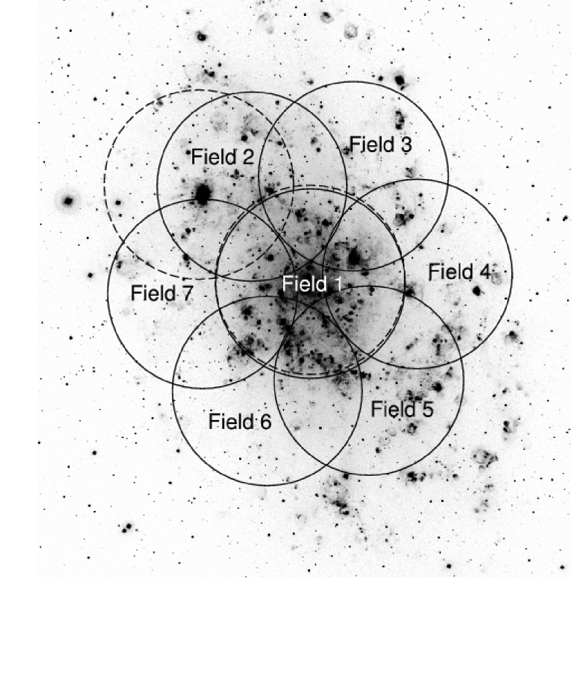
Figure 1.— Field of views of ChASeM33 pointings are plotted as 8′ circles (solid lines) on an ${\rm H}\alpha$ image from the Burrell Schmidt telescope on Kitt Peak (McNeil & Winkler, 2006). The ObsIDs 1730 and 2023 are shown as the circles with dashed lines.

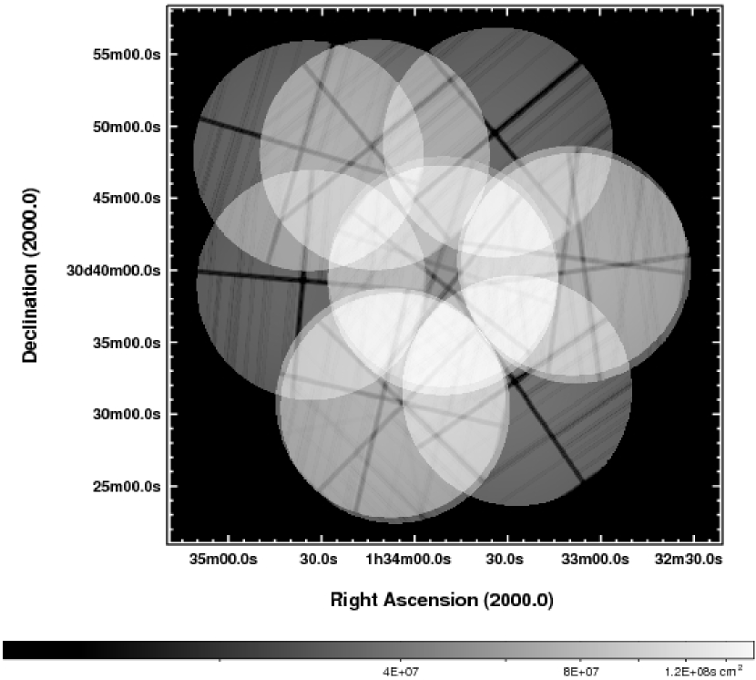
Figure 2.— Exposure map of all M 33 pointings with ACIS-I as the primary instrument (the ChASeM33 observations and OBSIDs 1730 and 2023) in units of ${\rm s~{}cm^{2}}$ , only including data with off-axis angles $<$ 8′. To compute the exposure map, spectral-weighted instrument maps were used as discussed in § 2.3.

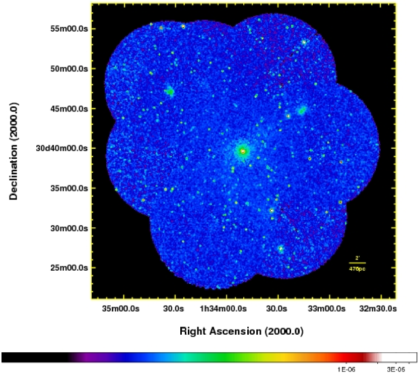
Figure 3.— Exposure-corrected mosaic image of all M 33 pointings with ACIS-I as the primary instrument (the ChASeM33 observations and OBSIDs 1730 and 2023) in units of ${\rm ct~{}cm^{-2}~{}s^{-1}}$, in the band 0.35 – 8.0 keV. Events within 8′ off-axis are used.

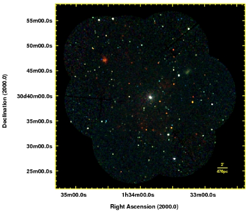
Figure 4.— Three-color mosaic image of all M 33 pointings with ACIS-I as the primary instrument (the ChASeM33 observations and OBSIDs 1730 and 2023), (red: 0.35 – 1.1 keV, green: 1.1 – 2.6 keV, and blue: 2.6 – 8.0 keV). Events are selected for off-axis angles $<8$′. The images are exposure corrected.

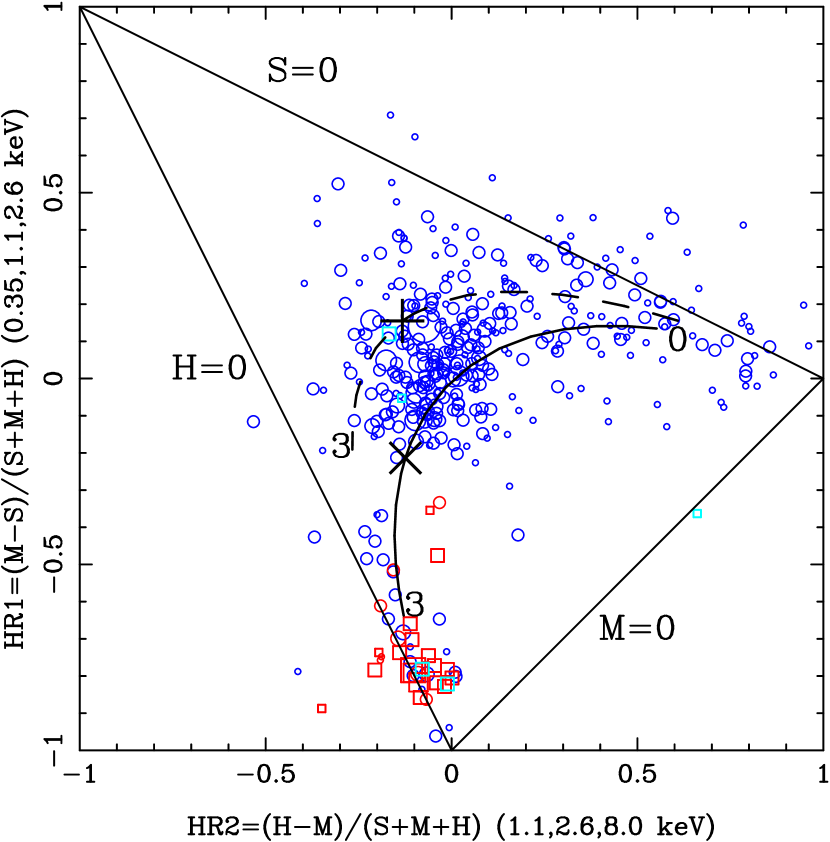
Figure 5.— Hardness radio plot constructed from the source list in Table 2. Unidentified sources are plotted in blue and GKL98 sources are plotted in red. Extended sources which are not in the GKL98 list are plotted as cyan. Sources are plotted as circles except for extended sources, which are plotted as squares. The symbol sizes indicate the approximate photon fluxes ($\mathrm{photons}\,\mathrm{cm}^{-2}\,\mathrm{s}^{-1}$): $<10^{-6}$ (smallest symbols), $10^{-6}$ to $10^{-5}$, $10^{-5}$ to $10^{-4}$, $10^{-4}$ to $10^{-3}$, and $>10^{-3}$ (largest symbols). The HR values are based on the photon fluxes and assume a flat spectrum to compute the mean effective area in the three bands. The black curves indicate the loci of power-laws with $\Gamma=0$–3 and with different $N_{\mathrm{H}}$: solid for $N_{\mathrm{H}}=1\times 10^{21}\,\mathrm{cm}^{-2}$, and dashed for $N_{\mathrm{H}}=3\times 10^{21}\,\mathrm{cm}^{-2}$. The large black $\times$ (+) indicate the $\Gamma=1.9$ powerlaw cases.

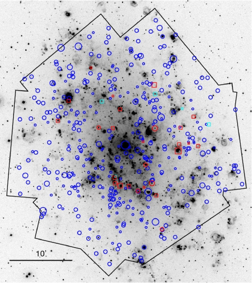
Figure 6.— Survey sources plotted on a deep ${\rm H}\alpha$ image taken with the Burrell Schmidt telescope at Kitt Peak (McNeil & Winkler 2006). Unidentified sources are plotted in blue, GKL98 sources are plotted in red and extended sources not in the GKL98 list are plotted in cyan; extended sources are plotted as squares, and the rest are plotted as circles. The symbol sizes encode the photon fluxes (see Fig. 5). The black polygon outlines the overall FOV of the overlapping ACIS-I FOVs of the survey.

Figure 7.— Chandra ACIS-I light curve of ChASeM33 #175 ([PMH04] 196) in the 0.5–2.5 keV band during ObsID 6383. Time zero corresponds to 15 June 2006 .

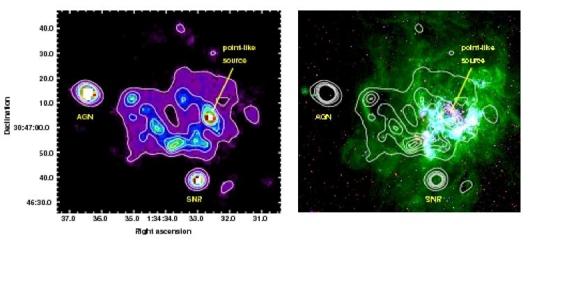
Figure 8.— Chandra ACIS-I image (left) and HST WFPC2 images (right) of the giant H ii region NGC 604 with Chandra contours (0.7, 1.2, 1.7, 2.2, and 2.7 counts/bin). The images cover $1\farcm 74\times 1\farcm 35$ region and 10″ corresponds to $\sim 40$ pc at the distance of M 33. The Chandra image is binned with a bin size of 2 pixels and smoothed using the FTOOL fadapt with a minimum of 20 cts in the kernel. In the right panel, HST $I$ band image is displayed in red, the ${\rm H}\alpha$ image in green, and the $V$ band image in blue.

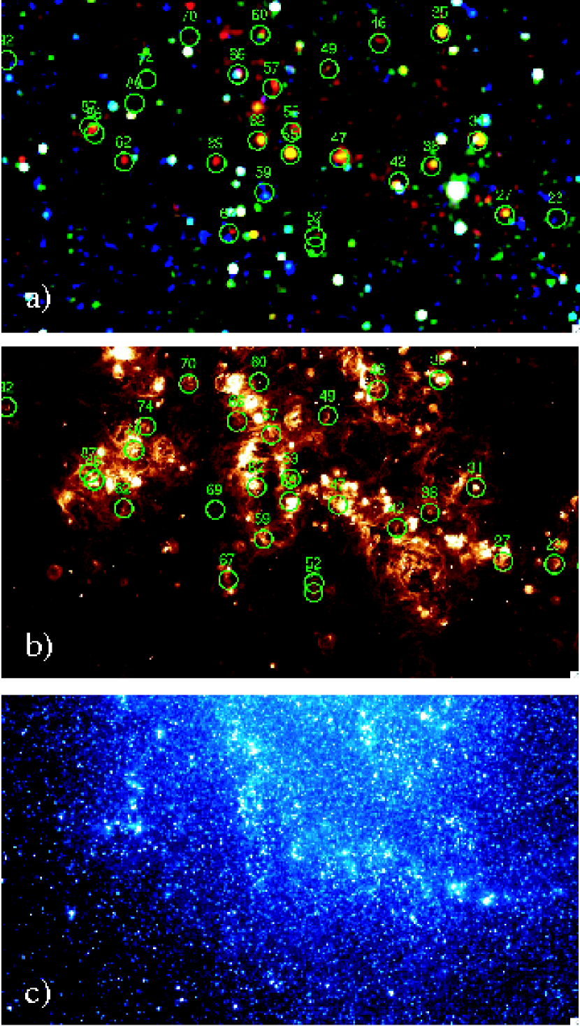
Figure 9.— A 9.3′ by 15.6′ region in the southern spiral arm of M 33 in three different wave bands. Panel a) shows a three-color image of the ChASeM33 data, with the soft band shown in red, medium band in green, and hard band in blue. Panel b) shows the LGGS ${\rm H}\alpha$ image after subtraction of the stellar background. Panel c) shows the Spitzer IRAC 3.6 $\mu$m image of the region, which is dominated by stellar light. SNRs from the GKL98 optical SNR catalog are indicated in the top two panels with 15″ diameter circles and ID numbers from that paper. Intensities are all shown on a log scale. Note the numerous coincidences of optical SNRs with soft Chandra sources in the southern spiral arm region.

References

- Broos et al. (2002) Broos, P. S., Townsley, L. K., Getman, K., & Bauer, F. E. 2002, ACIS Extract, An ACIS Point Source Extraction Package (University Park: Pennsylvania State Univ.) http://www.astro.psu.edu/xray/docs/TARA/ae_users_guide.html
- Calzetti et al. (1995) Calzetti, D., Kinney, A. L., Ford, H., Doggett, J., & Long, K. S. 1995, AJ, 110, 2739
- Ciardullo et al. (2004) Ciardullo, R., Durrell, P. R., Laychak, M. B., Herrmann, K. A., Moody, K., Jacoby, G. H., & Feldmeier, J. J. 2004, ApJ, 614, 167
- Colbert et al. (2004) Colbert, E. J. M., Heckman, T. M., Ptak, A. F., Strickland, D. K., & Weaver, K. A. 2004, ApJ, 602, 231
- Dickey & Lockman (1990) Dickey, J. M., & Lockman, F. J. 1990, ARA&A, 28, 215
- Eckart et al. (2006) Eckart, M. E., Stern, D., Helfand, D. J., Harrison, F. A., Mao, P. H., & Yost, S. A. 2006, ApJS, 165, 19
- Engargiola et al. (2003) Engargiola, G., Plambeck, R. L., Rosolowsky, E., & Blitz, L. 2003, ApJS, 149, 343
- Freedman et al. (2001) Freedman, W. L., et al. 2001, ApJ, 553, 47
- Freeman et al. (2002) Freeman, P. E., Kashyap, V., Rosner, R., & Lamb, D. Q. 2002, ApJS, 138, 185
- Gaetz et al. (2007) Gaetz, T. J., et al. 2007, ApJ, in press
- Garmire et al. (2003) Garmire, G. P., Bautz, M. W., Ford, P. G., Nousek, J. A., & Ricker, Jr., G. R. 2003, in X-Ray and Gamma-Ray Telescopes and Instruments for Astronomy. Edited by Joachim E. Truemper, Harvey D. Tananbaum. Proceedings of the SPIE, Volume 4851, pp. 28-44 (2003)., ed. J. E. Truemper & H. D. Tananbaum, 28–44
- Gehrels (1986) Gehrels, N. 1986, ApJ, 303, 336
- Ghavamian et al. (2005) Ghavamian, P., Blair, W. P., Long, K. S., Sasaki, M., Gaetz, T. J., & Plucinsky, P. P. 2005, AJ, 130, 539
- Gordon et al. (1998) Gordon, S. M., Kirshner, R. P., Long, K. S., Blair, W. P., Duric, N., & Smith, R. C. 1998, ApJS, 117, 89
- Grimm et al. (2005) Grimm, H.-J., McDowell, J., Zezas, A., Kim, D.-W., & Fabbiano, G. 2005, ApJS, 161, 271
- Haberl & Pietsch (2001) Haberl, F. & Pietsch, W. 2001, A&A, 373, 438
- Hatzidimitriou et al. (2006) Hatzidimitriou, D., Pietsch, W., Misanovic, Z., Reig, P., & Haberl, F. 2006, A&A, 451, 835
- Hong et al. (2004) Hong, J., Schlegel, E. M., & Grindlay, J. E. 2004, ApJ, 614, 508
- Long et al. (1996) Long, K. S., Charles, P. A., Blair, W. P., & Gordon, S. M. 1996, ApJ, 466, 750
- Long et al. (1981) Long, K. S., Dodorico, S., Charles, P. A., & Dopita, M. A. 1981, ApJ, 246, L61
- Maíz-Apellániz et al. (2004) Maíz-Apellániz, J., Pérez, E., & Mas-Hesse, J. M. 2004, AJ, 128, 1196
- Markert & Rallis (1983) Markert, T. H. & Rallis, A. D. 1983, ApJ, 275, 571
- Massey et al. (1996) Massey, P., Bianchi, L., Hutchings, J. B., & Stecher, T. P. 1996, ApJ, 469, 629
- Massey et al. (2002) Massey, P., Hodge, P. W., Holmes, S., Jacoby, J., King, N. L., Olsen, K., Smith, C., & Saha, A. 2002, Bulletin of the American Astronomical Society, 34, 1272
- Massey et al. (2006) Massey, P., Olsen, K. A. G., Hodge, P. W., Strong, S. B., Jacoby, G. H., Schlingman, W., & Smith, R. C. 2006, AJ, 131, 2478
- McNeil & Winkler (2006) McNeil, E. K. & Winkler, P. F. 2006, in Bull. AAS 39, 80
- Misanovic et al. (2006) Misanovic, Z., Pietsch, W., Haberl, F., Ehle, M., Hatzidimitriou, D., & Trinchieri, G. 2006, A&A, 448, 1247
- Newton (1980) Newton, K. 1980, MNRAS, 190, 689
- Park et al. (2003) Park, S., Hughes, J. P., Burrows, D. N., Slane, P. O., Nousek, J. A., & Garmire, G. P. 2003, ApJ, 598, L95
- Park et al. (2006) Park, T., Kashyap, V. L., Siemiginowska, A., van Dyk, D. A., Zezas, A., Heinke, C., & Wargelin, B. J. 2006, ApJ, 652, 610
- Pietsch et al. (2006a) Pietsch, W., Haberl, F., Sasaki, M., Gaetz, T. J., Plucinsky, P. P., Ghavamian, P., Long, K. S., & Pannuti, T. G. 2006a, ApJ, 646, 420
- Pietsch et al. (2006b) Pietsch, W., Plucinsky, P. P., Haberl, F., Shporer, A., & Mazeh, T. 2006b, The Astronomer’s Telegram, 905, 1
- Pietsch et al. (2005) Pietsch, W., Fliri, J., Freyberg, M. J., Greiner, J., Haberl, F., Riffeser, A., & Sala, G. 2005, A&A, 442, 879
- Pietsch et al. (2004) Pietsch, W., Misanovic, Z., Haberl, F., Hatzidimitriou, D., Ehle, M., & Trinchieri, G. 2004, A&A, 426, 11
- Pounds et al. (1994) Pounds, K. A., Nandra, K., Fink, H. H., & Makino, F. 1994, MNRAS, 267, 193
- Prestwich et al. (2003) Prestwich, A. H., Irwin, J. A., Kilgard, R. E., Krauss, M. I., Zezas, A., Primini, F., Kaaret, P., & Boroson, B. 2003, ApJ, 595, 719
- Sarajedina & Mancone (2007) Sarajedina, A. & Mancone, C. L. 2007, AJ, in press
- Schulman & Bregman (1995) Schulman, E. & Bregman, J. N. 1995, ApJ, 441, 568
- Stark et al. (1992) Stark, A. A., Gammie, C. F., Wilson, R. W., Bally, J., Linke, R. A., Heiles, C., & Hurwitz, M. 1992, ApJS, 79, 77
- Trinchieri et al. (1988) Trinchieri, G., Fabbiano, G., & Peres, G. 1988, ApJ, 325, 531
- Zaritsky et al. (1989) Zaritsky, D., Elston, R., & Hill, J. M. 1989, AJ, 97, 97