Influence of Zeeman splitting and thermally excited polaron states on magneto-electrical and magneto-thermal properties of magnetoresistive polycrystalline manganite $La_{0.8}Sr_{0.2}MnO_{3}$

Abstract

Some possible connection between spin and charge degrees of freedom in magneto-resistive manganites is investigated through a thorough experimental study of the magnetic (AC susceptibility and DC magnetization) and transport (resistivity and thermal conductivity) properties. Measurements are reported in the case of well characterized polycrystalline $La_{0.8}Sr_{0.2}MnO_{3}$ samples. The experimental results suggest rather strong field-induced polarization effects in our material, clearly indicating the presence of ordered FM regions inside the semiconducting phase. Using an analytical expression which fits the spontaneous DC magnetization, the temperature and magnetic field dependences of both electrical resistivity and thermal conductivity data are found to be well reproduced through a universal scenario based on two mechanisms: (i) a magnetization dependent spin polaron hopping influenced by a Zeeman splitting effect, and (ii) properly defined thermally excited polaron states which have to be taken into account in order to correctly describe the behavior of the less conducting region. Using the experimentally found values of the magnetic and electron localization temperatures, we obtain $L=0.5nm$ and $m_{p}=3.2m_{e}$ for estimates of the localization length (size of the spin polaron) and effective polaron mass, respectively.

I I. Introduction

Manganite systems exhibit a rich collection of interesting and intriguing properties, which can be tailored for a wide variety of applications (such as low-loss power delivery, quantum computing, ultra high-density magnetic data storage and more recently spintronic applications). Many such oxides have been prepared in bulk form or as thin films, which paved the way for intensive research studies in the past several decades (see, e.g.,  1 ; 2 ; 3 ; 4 ; 5 ; 6 ; 7 and further references therein). Among many different complex manganese oxides the most actively studied are the $(R_{1-x}A_{x})MnO_{3}$ series where $R(A)$ stands for a trivalent rare-earth (divalent alkaline-earth) cation.

It was the discovery of the so-called colossal magnetoresistance (CMR) in these materials that spurred their comprehensive and thorough study. Soon enough it was realized that CMR exhibiting materials possess many features which make them very fascinating. First of all, these compounds are found to undergo a distinctive double phase transition under cooling from a paramagnetic (PM) weakly conductive insulating-like (I) state to a ferromagnetic (FM) more conductive metallic-like (M) state. These two transitions occur at what is conveniently described as the Curie temperature $T_{C}$ and the so-called charge carrier localization temperature $T_{MI}$, respectively. The observable difference between the two critical temperature values is usually attributed to the quality of the sample. However, even for perfect (defect-free) single crystals these two temperatures are not exactly equal, due to inseparable correlations between charge and spin degrees of freedom which are admitted to be the causes behind the observable CMR phenomena. Besides, in real materials these interactions are always modified by both intrinsic and extrinsic inhomogeneities (for example, the parameters of both transitions are known to be very sensitive to the oxygen content).

Since no comprehensive theory which would explain all the complexity of this interesting phenomenon has been suggested so far, it is still very important to extract microscopic parameters from real measurements and compare them to theoretical forecasts. Many routes can be used to investigate or sort out the (likely) numerous (though basic) underlying mechanisms. It is now well established that the complicated phase diagram of magneto-resistive (MR) manganites is very sensitive to $Mn$ site substitution and to magnetic fields. Beyond the usually admitted primo scenarios (in terms of the double exchange mechanism), the structure sensitive Jahn-Teller effect and the strong electron-phonon coupling are found to play an important role in these materials 2 . Besides, in the low temperature conducting ferromagnetic phase, clear evidence for a collective magnon signature (in the form of the $T^{3/2}$ Bloch law) was found and attributed to the so-called magnon-polaron excitations 3 . It was also pointed out that while some features are better explained through localized (spin) states alone, others definitely require the presence of collective excitations (or both) for their explanation 1 ; 2 ; 3 . It would be also interesting to have complementary information, both away from and including the transition regions.

Some possible connection between spin and charge degrees of freedom in magneto-resistive manganites is sometimes investigated through either experimental studies of the magnetic properties or through transport properties. However for better understanding of the underlying physical mechanisms behind CMR like phenomena, it is always very important to study various properties quasi simultaneously. We strongly believe that experimental and theoretical results should corroborate and complement each other. That is why acquisition of fine reliable data (especially in the presence of strong magnetic fields) could help verify the modern theoretical concepts and allow to extract the values of important physical parameters with high precision. Moreover, in view of the intricate character of the interaction mechanisms involved, it is quite evident that some features will better manifest themselves via magneto-electric transport properties while the others will require more sophisticated magneto-thermal transport measurements.

In the present paper we endeavor to elucidate the field-induced charge-spin correlations in CMR exhibiting $La_{0.8}Sr_{0.2}MnO_{3}$ manganites previously studied by many researchers (a nonexhaustive list can be found in 4 ) through a thorough study of possible connections between their (equilibrium) magnetic and (non-equilibrium) transport properties. In achieving this goal, we have found new and somewhat unexpected results which, in our opinion, can shed more light on the nature of these interesting materials. The paper is organized as follows. In Section II we present the experimental results for our polycrystalline $La_{0.8}Sr_{0.2}MnO_{3}$ samples which include both magnetic (AC susceptibility and DC magnetization) and transport (resistivity and thermal conductivity) measurements in applied magnetic fields. A detailed theoretical discussion of the obtained results is given in Section III. To explain our findings, a universal and coherent scenario will be put forward based on various components, including (i) a magnetization dependent spin polaron hopping, (ii) Zeeman splitting effects, (iii) properly defined thermally excited polaron states (needed to correctly describe the temperature behavior of the less conducting region), and (iv) validity of the Wiedemann-Franz law. The paper is concluded with a short summary of the obtained results in Section IV.

II II. Experimental results

Polycrystalline $La_{0.8}Sr_{0.2}MnO_{3}$ samples were synthesized by a carbonate precursor method 5 . The structural quality of our samples was verified through X-ray diffraction. Structural refinements made with X-ray data show (see Fig. 1) that the samples are single phased and rhombohedral with structural parameters very close to the standard ones 6 ; 7 (with the oxygen deficiency less than $0.01$).

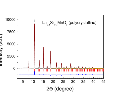
Figure 1: (Color online) Rietveld refinement plot for polycrystalline manganite of $La_{0.8}Sr_{0.2}MnO_{3}$: observed intensities (symbols: crosses), calculated intensities (wine line), background (yellow solid line), reflections (red vertical lines), and difference (blue solid line at the bottom).

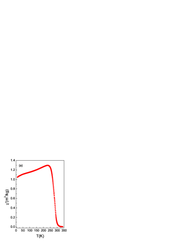
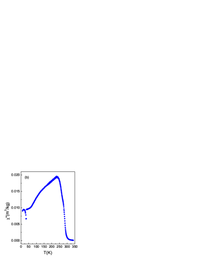
Figure 2: (Color online) Temperature dependence of (a) in-phase $\chi^{\prime}$ and (b) out-of-phase $\chi^{\prime\prime}$ components of the AC magnetic susceptibility of polycrystalline $La_{0.8}Sr_{0.2}MnO_{3}$.

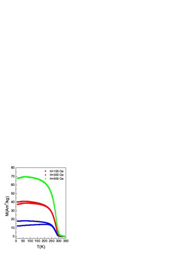
Figure 3: (Color online) Temperature dependence of DC magnetization of polycrystalline $La_{0.8}Sr_{0.2}MnO_{3}$ for various magnetic fields. The lower and upper branches correspond to zero-field-cooled (ZFC) and field-cooled (FC) curves, respectively.

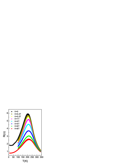
Figure 4: (Color online) Temperature dependence of electrical resistance of polycrystalline $La_{0.8}Sr_{0.2}MnO_{3}$ for various magnetic fields.

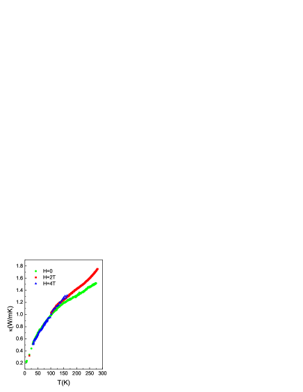
Figure 5: (Color online) Temperature dependence of thermal conductivity of polycrystalline $La_{0.8}Sr_{0.2}MnO_{3}$ for various magnetic fields.

Samples were magnetically characterized by measuring the temperature variation of magnetic AC susceptibility and DC magnetization at different applied magnetic fields. The temperature dependence of the in-phase component $\chi^{\prime}$ of the AC magnetic susceptibility reveals a typical ferromagnetic behavior with a very smooth decrease of $\chi^{\prime}$ below the maximum located near $231K$ (see Fig. 2(a)). The Curie temperature $T_{C}$ (defined by the largest slope of $\chi^{\prime}$) is equal to $286K$. The out-of-phase component $\chi^{\prime\prime}$ of the AC magnetic susceptibility (Fig. 2(b)) also exhibits a maximum around $231K$. It should be noted that an anomaly seen in the out-of-phase component (b) just below $50K$ is simply an artifact which arises from magnetic traces contained in a sample holder. It is reproducible but it is not related to the true manganite phase shown by the in-phase component (a). The temperature dependence of the DC magnetization under $100$, $300$ and $500Oe$ is shown in Fig. 3. For $H=100$ and $300Oe$ one may distinguish a pronounced split between the field-cooled (FC) and zero-field-cooled (ZFC) curves appearing below $230$ and $160K$, respectively. For $H=500Oe$ the FC and ZFC curves practically coincide. Such a weak irreversibility behavior suggests a rather low level of magnetic anisotropy in our sample. The Curie temperature gradually decreases from $T_{C}=284K$ (for $100Oe$) to $T_{C}=281K$ (for $500Oe$).

The electrical resistivity was measured by the standard four-probe method using currents up to $10mA$ (see 8 ; 9 ). The temperature dependence of the measured electrical resistivity (Fig. 4) is typical for magnetoresistive materials, exhibiting a two-phase behavior with a more conductive (metallic) and a less conductive (insulating) regions separated by a pronounced maximum at the peak temperature $T_{p}=204K$ (at zero magnetic field). Unlike the previously discussed Curie temperature variation, the resistance maximum gradually moves towards higher temperatures (approximately proportionally to the applied magnetic field) and reaches $T_{p}=217K$ at $H=8T$. This $T_{p}$ shift is accompanied by a marked reduction of the resistance maximum amplitude in the whole temperature range studied. The low temperature values of the resistivity at 8T are reduced almost three times as compared to the zero field case.

The thermal conductivity was measured using the stationary heat flux method 10 in the temperature range $5-300K$. The experimental setup and the measurement procedures have been described in detail earlier 10 ; 11 . The temperature gradient along the sample was in the range $0.1-0.5K$. The magnetic field was applied normally to the heat flow. Particular care was taken to avoid a parasitic heat transfer between the sample and its environment. The measurement error was below $2\%$ and the surplus error (estimated from the scattering of the measurement points) did not exceed $0.3\%$. Fig. 5 depicts the obtained temperature dependence of the thermal conductivity for various magnetic fields.

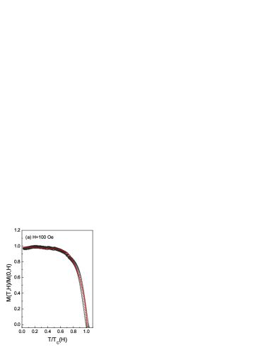
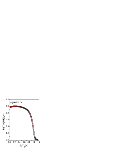
Figure 6: (Color online) The best fits (red solid lines) of the temperature dependence of the normalized magnetization $M(T,H)$ for (a) $H=100Oe$ and (b) $H=500Oe$, according to Eq.(1).

III III. Discussion

III.1 A. Magnetization

Let us start the discussion of the obtained results with thermodynamic properties and consider the behavior of a low-field DC magnetization $M(T,H)$ in the FM region. Fig. 6 shows the best fits of the temperature dependence of the normalized magnetization according to the following expression (which is an analytical approximate solution of the Curie-Weiss mean-field equations 12 )

$$M(T,H)=M_{ext}(H)+M_{0}(H)\tanh\left\{\sqrt{\left[\frac{T_{C}(H)}{T}\right]^{2}-1}\right\}$$ (1)

Here, $T_{C}(H)$ is the field-dependent Curie temperature, $M_{ext}(H)$ is external contribution to magnetization in applied field, and $M_{0}(H)$ accounts for deviation from the saturation value of spontaneous magnetization $M_{s}$. Using $T_{C}=286K$ and $T_{C}=281K$ for the experimentally found values of the Curie temperature for $H=100Oe$ and $H=500Oe$, respectively, the best fits produced $M_{0}=0.9M_{s}$ and $M_{ext}=0.1M_{s}$ for the model parameters.

Turning to the interpretation of the obtained results, notice that within the whole temperature interval, the sample is practically totally in a FM phase. Moreover, using a previously obtained phenomenological formula 13 $T_{MI}=(1-4M_{0}/9M_{s})T_{C}$ the found deviation from the saturation magnetization $M_{0}=0.9M_{s}$ thereby allows for an estimate of the M-I transition temperature $T_{MI}=0.6T_{C}$, which in turn provides to make a clear thermodynamic distinction between the metallic ($T<T_{MI}$) and semiconducting ($T>T_{MI}$) regions and complements the measured value of the resistivity peak temperature $T_{p}$ (discussed in the next Section).

III.2 B. Resistivity

Turning to the discussion of the transport properties in our polycrystalline samples, we notice that in order to exclude any extrinsic effects (like grain boundary scattering), it is more appropriate from a physical point of view to consider the normalized resistivity $\Delta\rho(T,H)/\Delta\rho(0,H)$ where $\Delta\rho(T,H)=\rho(T,H)-\rho(T_{p},H)$ with $T_{p}$ being the peak temperature and $\rho(0,H)$ the resistivity taken at the lowest available temperature. Fig. 7 depicts the above-defined normalized resistivity versus the reduced temperature $T/T_{p}(H)$ for (a) $H=0$, (b) $H=2T$, and (c) $H=4T$. The solid lines are the best fits to theoretical laws for which we outline the derivation in what follows. Let us start our discussion with a brief outlook of the polaron hopping conductivity scenarios. Recall that several 12 ; 13 ; 14 ; 15 ; 16 ; 17 ; 18 approaches have been suggested so far to tackle this problem. In essence, all of them are based on a magnetic localization concept which relates the observable MR at any temperature and/or applied magnetic field to the local magnetization. In particular, one of the most advanced models of this kind 15 ascribes the metal-insulator (M-I) like transition to a modification of the spin-dependent potential $J_{H}\vec{s}\cdot\vec{S}$ associated with the onset of magnetic order at $T_{C}$ (where $J_{H}$ is the on-site Hund’s-rule exchange coupling of an $e_{g}$ electron with $s=1/2$ to the localized $Mn$ $t_{2g}$ ion core with $S=3/2$). Specifically, the hopping based conductivity reads $\sigma(R)=\sigma_{0}(R)\exp[-U(R)]$ where $U(R)=2R/L-W_{ij}/k_{B}T$ and $\sigma_{0}(R)=e^{2}R^{2}\nu_{ph}N_{m}$. Here $R$ is the hopping distance (typically 12 , of the order of $1.5$ unit cells), $L$ the charge carrier localization length (typically 13 ; 17 , $L=0.5nm$), $\nu_{ph}$ the phonon frequency, $N_{m}$ the density of available states at the magnetic energy $J_{H}$, and $W_{ij}$ the effective barrier between the hopping sites $i$ and $j$. There are two possibilities to introduce an explicit magnetization dependence into the above model: either assuming a magnetization-dependent localization length $L(M)$ 16 which leads to an unusual thermal behavior of the electrical resistivity 12 ; 13 ; 18 or through modifying the hopping barrier assuming $W_{ij}=W_{ij}(M)$ 15 . The second scenario results in a more conventionally acceptable thermally activated behavior of MR over the whole temperature range. Indeed, since a sphere of radius $R$ contains $(4/3)\pi R^{3}/v$ sites where $v=5.7\times 10^{-29}m^{3}$ is the lattice volume per manganise ion, the smallest value of $W_{ij}$ is therefore $[(4/3)\pi R^{3}N(E_{m})]^{-1}$. Minimizing the hopping rate, one finds that the conductivity should vary according to the Mott law as follows

$$\sigma(T)=\sigma_{0}(T)\exp\left\{-\frac{T_{p}}{T}\left[1-\left(\frac{M}{M_{s}}\right)^{2}\right]\right\}^{1/4}$$ (2)

where

$$\sigma_{0}(T)=\sigma_{m}\sqrt{\frac{T_{p}}{T}}$$ (3)

with

$$\sigma_{m}=\left(\frac{4}{9}\right)e^{2}L^{2}\nu_{ph}N_{m}$$ (4)

and

$$T_{p}=\left(\frac{9}{4}\right)^{3}\frac{1}{2\pi k_{B}N_{m}L^{3}}$$ (5)

Notice that this scenario was used by Wagner et al. 17 to successfully interpret their MR data on low-conductive $Nd_{0.52}Sr_{0.48}MnO_{3}$ films.

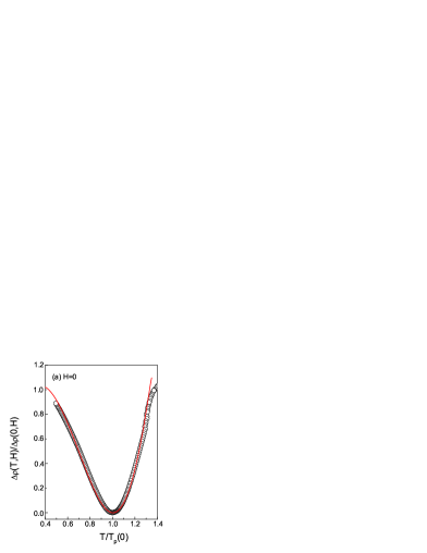
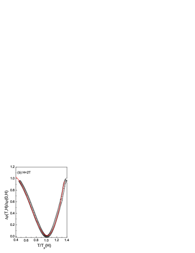
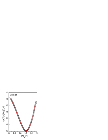
Figure 7: (Color online) Temperature dependence of the normalized resistivity $\Delta\rho(T,H)/\Delta\rho(0,H)$ versus the reduced temperature $T/T_{p}(H)$ for (a) $H=0$, (b) $H=2T$, and (c) $H=4T$. The red solid lines are the best fits according to the model equations (see the text).

Fig.7(a) presents the best fit for zero-field temperature dependence of the normalized resistivity $\Delta\rho(T,H)/\Delta\rho(0,H)$ according to our Eqs.(1)-(3) assuming as usual that $\rho=1/\sigma$. To make sure our scenario for spin polaron dominated transport makes sense indeed, let us estimate the ”vital” model parameters. In particular, using the typical value for the phonon frequency in this type of materials $\nu_{ph}=2\times 10^{13}s^{-1}$, and the experimental value for $\sigma_{m}$, our Eqs.(1)-(5) predict $L=0.5nm$ for the localization length (or the size of the spin polaron) in good agreement with the published values for this parameter 12 ; 13 ; 14 ; 15 ; 16 ; 17 ; 18 . Besides, using this found $L$ and the experimental value of the zero-field peak temperature $T_{p}=204K$, we get $N_{m}=2\times 10^{-28}m^{-3}eV^{-1}$ as a reasonable estimate of the carrier’s number density. Finally, using the experimental value of the zero-field Curie temperature $T_{C}=286K$, the spin exchange value of the coupling energy for our sample is estimated to be $J_{H}=25meV$ as is expected for this parameter 19 .

Turning to the influence of field effects on the temperature behavior of the resistivity in our sample, it is important to notice the different evolution of the two characteristic temperatures with the applied field $H$ which results in a marked modification of the boundary between the more conducting and less conducting regions. Indeed, while the peak temperature increases with $H$ reaching the value of $T_{p}=210K$ at $H=2T$, the Curie temperature, on the other hand, goes in the opposite direction, strongly decreasing from $T_{C}=286K$ at $H=0$ to $T_{C}=260K$ at $H=2T$. At the same time, a thorough analysis of the high-field results for the magneto-resistivity revealed that a simple modification of the hopping expression given by Eqs.(1)-(3) to non-zero magnetic fields is not enough to fit our MR data and some extra contribution is needed. Eventually, we found that our data for $H=2T$ and $H=4T$ shown in Fig.7(b) and Fig.7(c) can be quite successfully fitted assuming an appropriate field dependence of both critical temperatures, $T_{C}(H)$ and $T_{p}(H)$, and using the following expression

$$\sigma(T,H)=\sigma_{1}(T,H)+\sigma_{2}(T,H)$$ (6)

where $\sigma_{1}(T,H)$ is simply the field-induced hopping conductivity generalizing Eq.(2), that is

$$\sigma_{1}(T,H)=\sigma_{01}(T,H)\exp\left[-U_{1}(T,H)\right]$$ (7)

with

$$\sigma_{01}(T,H)=\sigma_{m1}\sqrt{\frac{T_{p}(H)}{T}}$$ (8)

and

$$U_{1}(T,H)=\left\{-\frac{T_{p}(H)}{T}\left[1-\left(\frac{M}{M_{s}}\right)^{2}\right]\right\}^{1/4}$$ (9)

Notice that the temperature and field dependence of DC magnetization $M(T,H)$ in the above equations is still governed by the universal expression given by Eq.(1). On the other hand, assuming a linear superposition of effects as in any linear response theory we propose the following empirical expression for an extra contribution to the magneto-conductivity

$$\sigma_{2}(T,H)=\sigma_{02}(T,H)[pe^{-U_{2}(T,H)}+(1-p)e^{+U_{2}(T,H)}]$$ (10)

where

$$\sigma_{02}(T,H)=\sigma_{m2}\left[\frac{T}{T_{0}(H)}\right]^{1/4}$$ (11)

and

$$U_{2}(T,H)=\frac{T}{T_{0}(H)}$$ (12)

Let us consider the origin of the $\sigma_{2}(T,H)$ term in the total MR in our material. As a matter of fact, the very form of Eq.(10) suggests that this contribution describes equilibrium state of a two-level system (with fractional population $p$) created by spin-dependent energy splitting in applied magnetic field 20 . More specifically, this contribution is governed by a Zeeman like term $W_{H}=-\mu(R)H$ where $\mu(R)=\pi R^{2}gS\mu_{B}L/v$ is the local magnetic moment of spin polaron 21 . Here, $R$ is the hopping distance, $v$ is the lattice volume per manganite ion, $\mu_{B}$ is the Bohr magneton and $g$ is the gyromagnetic ratio. It should be noted that unlike the previous contribution, given by the $\sigma_{1}(T,H)$ term, the second contribution does not exhibit a thermally-activated behavior even though (as we shall see) it is still related to the adopted in this paper spin polaron hopping scenario.

Furthermore, to correctly describe the semiconducting region (above $T_{MI}=0.77T_{C}$), it is important to take into account thermally excited polaron states 22 with the number density $n(T)=(2\pi m_{p}k_{B}T/\hbar^{2})^{3/2}$ where $m_{p}$ is an effective polaron mass.

Based on the above assumptions, the second contribution to the transport mechanism in our material can be presented in the general form of a field-dependent hopping conductivity as follows:

$$\sigma_{2}(R,H)=\sigma_{02}(R)[pe^{-U_{2}(R,H)}+(1-p)e^{+U_{2}(R,H)}]$$ (13)

where

$$U_{2}(R,H)=\frac{2R}{L}-\frac{\mu(R)H}{k_{B}T}$$ (14)

and

$$\sigma_{02}(R)=e^{2}R^{2}\nu_{ph}N_{s}(R,T)$$ (15)

Here $N_{s}(R,T)=\sqrt{n(T)/N(R)J_{H}^{2}v}$ is the local number density of polaron states (including thermally excited carriers in the semiconducting region) with $N(R)=3\pi R^{3}/4v$ being the number of available sites.

Minimizing the hopping rate given by Eqs. (13)-(15), we find that the second contribution to the MR is indeed governed by Eqs.(10)-(12) with

$$\sigma_{m2}(H)=e^{2}L^{2}\nu_{ph}\left(\frac{2m_{p}}{h^{2}L^{2}}\right)^{3/4}\left[\frac{36\pi^{2}}{k_{B}T_{0}(H)}\right]^{1/4}$$ (16)

and

$$T_{0}(H)=\frac{4\pi L^{3}gS\mu_{B}H}{k_{B}v}$$ (17)

Using $T_{C}=260K$ and $T_{p}=210K$ for the experimentally found values of the Curie temperature and the resistivity peak temperature at $H=2T$, respectively, the best fits were obtained for the following set of the model parameters: $T_{0}=240K$, $M_{ext}=0.47M_{s}$, $M_{0}=0.53M_{s}$, and $p=0.72$. Furthermore, since 13 $T_{MI}=(1-4M_{0}/9M_{s})T_{C}$ the above deviation from the saturation magnetization gives $T_{MI}=0.77T_{C}$ for an estimate of the M-I transition temperature at $H=2T$ (to be compared with $T_{MI}=0.6T_{C}$ at $H=0$). Along with a similar behavior of the peak temperature $T_{p}$, this implies an effective extension of the more conductive phase to higher temperatures (in contrast with the field-free case shown in Fig.7(a)). Using the previously discussed values of the phonon frequency $\nu_{ph}$, the size of the spin polaron (localization length) $L$, and the experimental values for $\sigma_{m1}$ and $\sigma_{m2}$, from Eqs. (16) and (17) we obtain $m_{p}=3.2m_{e}$ for a reasonable estimate of the effective polaron mass 2 . Furthermore, let us estimate the absolute values of the Curie temperature $T_{C}(H)$ and the electron temperature $T_{MI}(H)$ for $H=2T$. Making a reasonable assumption that $k_{B}T_{C}(H)=k_{B}T_{C}(0)-\mu(L)H$ with $k_{B}T_{C}(0)=J_{H}=25meV$ being a zero-field value and $\mu(R)$ being defined earlier, we find $k_{B}T_{C}(H)=20meV$ or $T_{C}(H)=260K$, in agreement with the observations. Likewise, the field dependence of $T_{MI}(H)$ is governed by the corresponding behavior of the density of polaron states as follows $T_{MI}(H)\propto 1/N_{m}[J_{H}-\mu(L)H]$. Since $\mu(L)H/J_{H}\ll 1$, we find that $T_{MI}(H)\simeq T_{MI}(0)[1+\mu(L)H/J_{H}]$ where $T_{MI}(0)\propto 1/N_{m}(J_{H})$, so that $T_{MI}(H)=200K$.

Finally, it is worth commenting on the value of the fractional population $p$. In magnetically disordered well-defined paramagnetic phase one would expect equal distribution of populations of spin polarons with $p=1/2$. The fact that our experiments instead predict $p=0.72$ suggests rather strong field-induced polarization effects at $H=2T$ in our material, indicating the presence of ordered FM regions in the semiconducting phase as well.

III.3 C. Thermal conductivity

Based on the above experimental background and our previous experience in studying thermoelectric response of similar class of materials 13 , it is quite reasonable to assume that the heat transport properties of our sample are dominated by hopping (tunneling) of spin polarons and a Zeeman term as well. When discussing the relationship between electric and heat transport behavior in both metallic and non-metallic systems, the main question which always needs to be addressed (and still remains controversial) is about the validity of the so-called Wiedemann-Franz (WF) law. For example, a recent report by Lia et al. 14 suggests that the ratio of the thermal conductivity to the electrical conductivity in their $Nd_{0.75}Na_{0.25}MnO_{3}$ samples strongly deviates from the WF law even in the FM metallic state. Our present study, on the other hand, seems to be in total support of the WF law for the whole temperature interval because, based on the above assumptions, we are able to successfully fit our zero-field data for the thermal conductivity shown in Fig. 8(a) using the following expression (Cf. with similar Eqs.(2)-(9) for the resistivity)

$$\kappa(T)=\kappa_{0}(T)\exp\left[-U(T)\right]$$ (18)

where

$$\kappa_{0}(T)=\kappa_{m}\sqrt{\frac{T}{T_{p}}}$$ (19)

and

$$U(T)=\left\{-\frac{T_{p}}{T}\left[1-\left(\frac{M}{M_{s}}\right)^{2}\right]\right\}^{1/4}$$ (20)

The direct comparison with Eq.(3) reveals that our fitting expression for the pre-factor $\kappa_{0}(T)$ given by Eq.(19) is nothing else but a manifestation of the WF law relating the electric and thermal conductivities because

$$\kappa_{0}(T)=\frac{\pi^{2}k_{B}^{2}T}{3e^{2}}\sigma_{0}(T)=\kappa_{m}\sqrt{\frac{T}{T_{p}}}$$ (21)

with

$$\kappa_{m}=\frac{27\pi k_{B}\nu_{ph}}{32L}$$ (22)

Likewise, high-field results for the thermal conductivity are found to be well described using the field-induced modification of hopping scenario assuming the validity of the WF law. Namely, Fig. 8(b) and Fig. 8(c) show the best fits for $H=2T$ and $H=4T$ using the following expression which takes into account both hopping ($\kappa_{1}$) and Zeeman ($\kappa_{2}$) terms

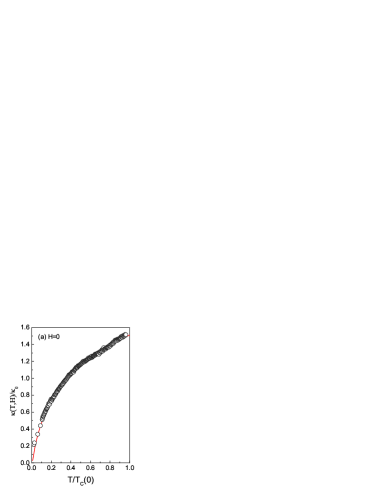
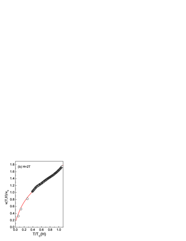
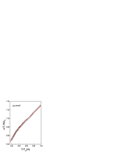
Figure 8: (Color online) Temperature dependence of the thermal conductivity $\kappa(T,H)/\kappa_{0}$ versus the reduced temperature $T/T_{C}(H)$ for (a) $H=0$, (b) $H=2T$, and (c) $H=4T$. The red solid lines are the best fits according to the model equations (see the text).

$$\kappa(T,H)=\kappa_{1}(T,H)+\kappa_{2}(T,H)$$ (23)

where

$$\kappa_{1}(T,H)=\kappa_{01}(T,H)\exp\left[-U_{1}(T,H)\right]$$ (24)

with

$$\kappa_{01}(T,H)=\frac{\pi^{2}k_{B}^{2}T}{3e^{2}}\sigma_{01}(T,H)=\kappa_{m1}\sqrt{\frac{T}{T_{p}(H)}}$$ (25)

while a Zeeman-type two-level induced contribution reads (similarly to Eq.(10))

$$\kappa_{2}(T,H)=\kappa_{02}(T,H)[pe^{-U_{2}(T,H)}+(1-p)e^{+U_{2}(T,H)}]$$ (26)

where

$$\kappa_{02}(T,H)=\frac{\pi^{2}k_{B}^{2}T}{3e^{2}}\sigma_{02}(T,H)=\kappa_{m2}\left[\frac{T}{T_{0}(H)}\right]^{1/4}$$ (27)

with

$$\kappa_{m2}(H)=\sqrt{\frac{\pi^{2}}{12}}\left(\frac{k_{B}\nu_{ph}}{L}\right)\left[\frac{2m_{p}k_{B}T_{0}(H)L^{2}}{\hbar^{2}}\right]^{3/4}$$ (28)

and with $T_{0}(H)$ still given by Eq.(17). It is important to note that the best fits for the magneto-thermal conductivity were obtained for the set of model parameters used in the previous Section for fitting of our magneto-resistivity data. In particular, the $H=2T$ data were fitted using: $T_{C}=260K$, $T_{p}=210K$, $T_{0}=240K$, $M_{ext}=0.47M_{s}$, $M_{0}=0.53M_{s}$, and $p=0.72$.

IV IV. Conclusions

It was pointed out 23 ; 24 on investigations of magnetotransport in charge ordered manganites with similar magnetic ground states that the origin of magnetoresistance cannot be concluded from the isofield resistivity measurements alone. Hence it is of importance to organize experimental runs on related properties (equilibrium and nonequilibrium ones) quasi simultaneously on the same materials. Moreover it was found that neutron spectra of CMR materials cannot be usually explained with a picture of spin clusters moving in a paramagnetic background (i.e. magnetic polarons). Rather, a model describing an average magnetic coherence extending over several $Mn$ spins leads to better fits to the data (see Viret et al. 4 ). That is why it is interesting to examine a possible interplay between different magnetic states including both localized and collective excitations. In Ref. 3 , some regimes had already been pointed out through similarities (and differences) between the specific heat data and the electrical resistivity. In order to further shed some light on a possible connection between spin and charge degrees of freedom in CMR exhibiting manganites, a thorough experimental study of two magnetic and two transport properties of magneto-resistive polycrystalline $La_{0.8}Sr_{0.2}MnO_{3}$ samples has been presented in this paper. Using a properly generalized analytical expression for the spontaneous DC magnetization [Eq.(1)], the temperature and magnetic field dependencies of electrical resistivity [Eq.(6)] and thermal conductivity [Eq.(23)] were successfully fitted, assuming spin polaron hopping scenario (strongly influenced by a Zeeman type splitting effects), presence of thermally excited polaron states (needed to correctly describe the semiconducting region), and the validity of the Wiedemann-Franz law. It is important to underline the self-consistency and coherence of our approach which produced very reasonable estimates for numerical values of microscopic parameters. It is also worth noting that the presented experimental and theoretical results corroborate magneto-transport measurements and subsequent analysis on the temperature behavior of previously obtained magneto-thermopower results on a similar material 13 . And finally, a brief comment is in order on the role of grain-boundary effects in the transport properties under discussion. The very fact that the adopted here polaron picture reasonably well describes both electric resistivity and thermal conductivity suggests a rather high quality of our sample (which is also evident from its X-ray diagram shown in Fig.1) with presumably narrow enough grain distribution and quasi-homogeneous low-energy barriers between the adjacent grains. Besides, in order to minimize the inevitable influence of the grain-boundary scattering effects on the metal-insulator transition temperature in polycrystalline samples (see, e.g., 25 for detailed discussion), the latter is defined via the properly normalized resistivity data (see Fig. 7).

Note added: when our paper was completed, we became aware of the very important experimental results on direct observation of polaron states and nanometer-scale phase separation in CMR exhibiting manganites. More specifically, using high resolution topographic images obtained by scanning tunneling microscope, regular stripe-like or zigzag patterns on a width scale ranging between $0.4nm$ and $0.5nm$ were observed 26 in the insulating state of $Pr_{0.68}Pb_{0.32}MnO_{3}$ which remarkably correlate with the size of spin polarons ($L=0.5nm$) deduced from our present measurements on $La_{0.8}Sr_{0.2}MnO_{3}$ providing thus further evidence in support of our interpretation based on spin polaron scenario.

V acknowledgments

This work was partially supported by Brazilian agency CAPES, Ministry of Science and Higher Education (PL) - grant Walonia/286/2006, Kasa Mianowskiego (PL), CGRI (B) and FNRS (B) in Liege through B 8/5-CB/SP-9.154 and FRFC 1.5.115.03 convention.

References

-
(1)
E. Dagotto, T. Hotta, and A. Moreo, Phys. Rep. 344, 1
(2001);
E. Dagotto, Nanoscale Phase Separation and Colossal Magnetoresistance: The Physics of Manganites and Related Compounds (Springer-Verlag, Heidelberg, 2003).
-
(2)
M.B. Salamon, Rev. Mod. Phys. 73, 583 (2001).
-
(3)
M. Ausloos, L. Hubert, S. Dorbolo, A. Gilabert, and R. Cloots, Phys. Rev. B 66, 174436
(2002).
-
(4)
H.Y. Hwang, S.W. Cheong, N. P. Ong, and B. Batlogg, Phys. Rev. Lett. 77, 2041
(1996);
P.E. Lofland, S.M. Bhagat, K. Ghosh, R.L. Greene, S.G. Karabashev, D.A. Shulyatev, A.A. Arsenov, and Y. Mukovskii, Phys. Rev. B 56, 13705 (1997);
M. Viret, H. Glattli, C. Fermon, A.M. de Leon-Guevara, and A. Revcolevschi, Europhys. Lett. 42, 301 (1998);
W. Westerburg, F. Martin, P.J.M. van Bentum, J.A.A.J. Perenboom, and G. Jakob, Eur. Phys. J. B 14, 509 (2000);
M. Auslender, A.E. Kar’kin, E. Rozenberg, and G. Gorodetsky, J. App. Phys. 89, 6639 (2001);
A.N. Ulyanov, I.S. Maksimov, E.B. Nyeanchi, Seong-Cho Yu, Yu.V. Medvedev, N.Yu. Starostyuk, and B. Sundqvist, J. Phys. Soc. Japan 71, 927 (2002);
X.-J. Liu, Y. Moritomo, A. Nakamura, H. Tanaka, and T. Kawai , J. Phys. Soc. Japan 70, 3466 (2002);
O. Chmaissem, B. Dabrowski, S. Kolesnik, J. Mais, J.D. Jorgensen, and S. Short, Phys. Rev. B 67, 094431 (2003);
-
(5)
M. Pekala, V. Drozd, and J. Mucha, J. Mag. Magn. Mater. 290-291, 928
(2005).
-
(6)
A. Urushibara, Y. Moritomo, T. Arima, A. Asamitsu, G. Kido, and Y. Tokura, Phys. Rev. B 51, 14103
(1995).
-
(7)
J.F. Mitchell, D.N. Argyriou, C.D. Potter, D.G. Hinks, J.D. Jorgensen, and S.D. Bader,
Phys. Rev. B 54, 6172 (1996).
-
(8)
M. Ausloos, M. Pekala, J. Latuch, J. Mucha, Ph. Vanderbemden, and R. Cloots,
J. Appl. Phys. 96, 7338 (2004).
-
(9)
M. Pekala, J. Mucha, B. Vertruyen, R. Cloots, and M. Ausloos, J. Magn. Magn. Mater. 306, 181
(2006).
-
(10)
A. Jezowski, J. Mucha, and G. Pompe, J. Phys. D: Appl. Phys. 201, 1500
(1987).
-
(11)
J. Mucha, S. Dorbolo, H. Bougrine, K. Durczewski, and M. Ausloos, Cryogenics 44, 145
(2001).
-
(12)
S. Sergeenkov, H. Bougrine, M. Ausloos, and R. Cloots, JETP Lett. 69, 858
(1999).
-
(13)
S. Sergeenkov, H. Bougrine, M. Ausloos, and A. Gilabert, Phys. Rev. B 60, 12322
(1999).
-
(14)
Z.Q. Lia, X.H. Zhang, W.R. Li, W. Song, H. Liu, P. Wu, H.L. Bai, and E.Y. Jiang,
Physica B 371, 177 (2006).
-
(15)
M. Viret, L. Ranno, and J.M.D. Coey, Phys. Rev. B 55, 8067
(1997).
-
(16)
L. Sheng, D.Y. Xing, D.N. Sheng, and C. S. Ting, Phys. Rev. Lett. 79, 1710
(1997).
-
(17)
P. Wagner, I. Gordon, L. Trappeniers, J. Vanacken, F. Herlach, V.V. Moshchalkov, and Y. Bruynseraede,
Phys. Rev. Lett. 81, 3980 (1998).
-
(18)
S. Sergeenkov, M. Ausloos, H. Bougrine, A. Rulmont, and R. Cloots, JETP Lett. 70,
481 (1999).
-
(19)
W.E. Pickett and D.J. Singh, Phys. Rev. B 53, 1146 (1996).
-
(20)
Ch. Kittel, Introduction to Solid State Physics (John Wiley and Sons, New
York, 1996).
-
(21)
X.J. Chen, H.-U. Habermeier, C.L. Zhang, H. Zhang, and C.C. Almasan, Phys. Rev. B 67, 134405
(2003).
-
(22)
B.I. Shklovskii and A.I. Efros, Electronic Properties of Doped Semiconductors (Springer, Berlin,
1984).
-
(23)
R. Mahendiran, A. Maignan, C. Martin, M. Hervieu, and B. Raveau, Phys. Rev. B 62, 11644
(2000).
-
(24)
B. Raveau, J. Mater. Chem. 8, 1405 (1998);
B. Raveau, M. Hervieu, A. Maignan, and C. Martin, J. Mater. Chem. 11, 29 (2001);
B. Raveau, A. Maignan, C. Martin, and M. Hervieu, J. Supercond. 12, 247 (2004).
-
(25)
Y. Tokura and Y.Tomioka, J. Mag. Magn. Mater. 200, 1 (1999).
- (26) Sahana Rößler, S. Ernst, B. Padmanabhan, Suja Elizabeth, H.L. Bhat, F. Steglich, and S. Wirth, http://arXiv.org/abs/cond-mat/07054243, submitted for publication.