Non-equilibrium hydrogen ionization in 2D simulations of the solar atmosphere.

Abstract

Context. The ionization of hydrogen in the solar chromosphere and transition region does not obey LTE or instantaneous statistical equilibrium because the timescale is long compared with important hydrodynamical timescales, especially of magneto-acoustic shocks. Since the pressure, temperature, and electron density depend sensitively on hydrogen ionization, numerical simulation of the solar atmosphere requires non-equilibrium treatment of all pertinent hydrogen transitions. The same holds for any diagnostic application employing hydrogen lines.

Aims. To demonstrate the importance and to quantify the effects of non-equilibrium hydrogen ionization, both on the dynamical structure of the solar atmosphere and on hydrogen line formation, in particular H $\alpha$.

Methods. We implement an algorithm to compute non-equilibrium hydrogen ionization and its coupling into the MHD equations within an existing radiation MHD code, and perform a two-dimensional simulation of the solar atmosphere from the convection zone to the corona.

Results. Analysis of the simulation results and comparison to a companion simulation assuming LTE shows that: a) Non-equilibrium computation delivers much smaller variations of the chromospheric hydrogen ionization than for LTE. The ionization is smaller within shocks but subsequently remains high in the cool intershock phases. As a result, the chromospheric temperature variations are much larger than for LTE because in non-equilibrium, hydrogen ionization is a less effective internal energy buffer. The actual shock temperatures are therefore higher and the intershock temperatures lower. b) The chromospheric populations of the hydrogen $n\!=\!2$ level, which governs the opacity of H$\alpha$, are coupled to the ion populations. They are set by the high temperature in shocks and subsequently remain high in the cool intershock phases. c) The temperature structure and the hydrogen level populations differ much between the chromosphere above photospheric magnetic elements and above quiet internetwork. d) The hydrogen $n\!=\!2$ population and column density are persistently high in dynamic fibrils, suggesting that these obtain their visibility from being optically thick in H $\alpha$ also at low temperature.

1 Introduction

The chromosphere represents the least understood regime of the sun (Judge & Peter 1998). In this paper we address the treatment of hydrogen ionization in simulations of the solar chromosphere. It is of paramount importance because hydrogen makes up 90% of the nuclei in the solar atmosphere, is an important and often dominant electron donor, and contains a large part of the internal energy of the gas. Hence, the ionization state of hydrogen strongly influences the temperature, pressure and electron density. Radiation magnetohydrodynamic (MHD) simulations of the atmosphere must therefore account properly for hydrogen ionization. This is not only important for the structure of the atmosphere within a simulation, but also for subsequent computation of the emergent spectrum from the simulation for comparison with observations.

Klein et al. (1976, 1978) and Kneer (1980) already showed from idealized one-dimensional (1D) models that the assumption of instantaneous statistical equilibrium (SE) for hydrogen ionization does not hold in a dynamical atmosphere containing shock waves. The temperature difference between the hot shocks and the cool intershock phases produces disparate ionization and recombination timescales, the latter being far slower than the former.

Carlsson & Stein (1992, 1995, 2002) computed dynamical 1D simulations of the solar atmosphere including a detailed non-equilibrium treatment of the hydrogen rate equations including ionization and recombination (i.e. not instantaneous statistical equilibrium but employing pertinent time derivatives in the population rate equations, as in Appendix A of the present paper). In the first paper they showed that the non-equilibrium effects lead to significant increase in shock temperature compared with the case of instantaneous LTE ionization and recombination. In the second paper they supply a detailed analysis of the hydrogen ionization in their simulations. They found that the chromospheric hydrogen ionization/recombination timescale is of the order of 50 s within hot shocks and $10^{3}-10^{5}$ s in the cool intershock regions, and that hydrogen becomes partially ionized within shocks but, owing to the long recombination timescale, does not recombine in the subsequent post-shock phase. As a consequence, the degree of ionization of hydrogen in the chromosphere is rather constant with time, in stark contrast to what the classical assumptions of statistical equilibrium or LTE would predict.

The present limitations on computing power do not yet permit such full-fledged non-equilibrium treatment of hydrogen ionization including radiative transfer in 2D and 3D simulation geometry. Therefore, approximations remain necessary to make the problem computationally tractable. In this work we employ the method formulated by Sollum (1999).

Sollum showed that in 1D dynamical modeling it is possible to avoid detailed evaluation of the radiation field in the relevant hydrogen transitions by prescribing suitable radiative rates. He found that this approximation works well up to just below the transition region. Sollum’s method is fast enough for use in multi-dimensional geometry. It was earlier implemented in the code CO⁵BOLD (Freytag et al. 2002) to perform a 3D non-magnetic hydrodynamical simulation of the chromosphere by Leenaarts & Wedemeyer-Böhm (2006). This simulation confirmed the conclusion obtained by Carlsson & Stein (1992, 2002) from 1D simulation: the degree of hydrogen ionization in the middle and upper chromosphere is determined by the passage of high-temperature shocks, irrespective of the cool intershock phases. It is relatively constant at about $10^{-3}$ to $10^{-2}$. However, Leenaarts & Wedemeyer-Böhm (2006) did not implement back-coupling of the non-equilibrium ionization into the equation of state for the gas within the hydrodynamical simulation. This is difficult to do in the CO⁵BOLD code because it employs an approximate Riemann solver for the hydrodynamics.

In this paper we first present our implementation of Sollum’s method including back-coupling of the non-equilibrium ionization into the equation of state in the Oslo MHD code described by Hansteen (2004) which uses a finite difference scheme for the hydrodynamics. We then discuss an extensive 2D simulation of chromospheric fine-structure evolution with this code and analyze the results in terms of the hydrogen ionization balance, with separation between the chromospheric behavior above a magnetic element and in an area resembling quiet-sun internetwork. The effects of non-equilibrium hydrogen ionization are demonstrated quantitatively through comparison with a similar companion simulation. The latter was started with identical initial conditions but its hydrogen ionization was set to obey LTE, i.e. instantaneous Saha–Boltzmann partitioning.

2 Method

In this section we describe our implementation of Sollum’s method in the MHD code developed in Oslo (Hansteen 2004). This code is based on the staggered grid code described in Dorch & Nordlund (1998), Mackay & Galsgaard (2001) and by Galsgaard & Nordlund. It includes the multi-group opacity-binning method of Nordlund (1982) and the treatment of scattering of Skartlien (2000) for radiative transfer in the photosphere and chromosphere. In the transition region and corona it employs optically thin radiative cooling. In addition, it treats radiative losses in strong lines and continua of hydrogen and Ca II in the upper chromosphere and transition region using an approximation based on detailed 1D computation with the RADYN code of Carlsson & Stein (1992). Thermal conduction along magnetic field lines is taken into account (Hansteen 2004).

In this section we first summarize the temporal evolution scheme of the MHD algorithm and then specify the modifications through which we insert non-equilibrium hydrogen ionization, the boundary conditions, and our simulation setup.

2.1 MHD evolution scheme

The MHD solver is the explicit third-order predictor-corrector scheme developed by Hyman (1979) but modified to allow variable timesteps. Its fundamental variables are the density $\rho$, momentum $\@vec{p}$, internal energy density $e_{\mathrm{i}}$ and the magnetic field $\@vec{B}$. The evolution equations for the fundamental variables depend only on the variables themselves, the temperature, the gas pressure, and their spatial derivatives. These derivatives are computed using a sixth-order scheme. The temperature and pressure are looked up in precomputed tables as function of density and internal energy. This table is computed assuming LTE except where the density and internal energy have typical coronal values. There coronal equilibrium is assumed.

The evolution equation for fundamental variable $f$ is

$$\frac{\partial f(t)}{\partial t}=\dot{f}$$ (1)

where $\dot{f}$ only depends on quantities known at time $t$. Hyman’s scheme solves this equation from timestep $n$ to timestep $n+1$ as follows: the predictor step is

$$f^{(*)}_{n+1}=a_{1}f_{n-1}+(1-a_{1})f_{n}+b_{1}\dot{f}_{n},$$ (2)

and the corrector step

$$f_{n+1}=a_{2}f_{n-1}+(1-a_{2})f_{n}+b_{2}\dot{f}_{n}+c_{2}\dot{f}^{(*)}_{n+1},$$ (3)

where $a_{1}$, $a_{2}$, $b_{1}$, $b_{2}$ and $c_{2}$ are coefficients that depend on the current and previous timestep sizes.

2.2 Implementation of non-equilibrium hydrogen ionization

In order to compute non-equilibrium hydrogen ionization one has to solve the hydrogen rate equations

$$\frac{\partial n_{i}}{\partial t}+\nabla\cdot(n_{i}\@vec{v})=\sum_{j,j\neq i}^{n_{{\rm l}}}n_{j}P_{ji}-n_{i}\sum_{j,j\neq i}^{n_{{\rm l}}}P_{ij},$$ (4)

where $n_{i}$ is the population of hydrogen level $i$, $\@vec{v}$ the macroscopic velocity, $n_{{\rm l}}$ the number of levels and $P_{ij}$ the transition rate coefficient between levels $i$ and $j$. The left-hand side represents a continuity equation for the hydrogen populations, the right-hand side a source term describing the transitions between the hydrogen levels. These equations are solved using operator splitting. The continuity part

$$\frac{\partial n_{i}}{\partial t}=-\nabla\cdot(n_{i}\@vec{v})$$ (5)

is solved using Hyman’s scheme in tandem with the fundamental variables. It is not possible to use sixth-order spatial derivatives for the hydrogen populations because negative populations then arise occasionally from the steep gradients in the population densities. Instead, a positive-definite first-order upwind scheme is used to ensure positivity of the populations.

After the predictor step, the rate part of the equations,

$$\frac{\partial n_{i}}{\partial t}=\sum_{j,j\neq i}^{n_{{\rm l}}}n_{j}P_{ji}-n_{i}\sum_{j,j\neq i}^{n_{{\rm l}}}P_{ij},$$ (6)

is integrated over the timestep $\Delta t$ while enforcing charge conservation, hydrogen nuclei conservation, energy conservation and instantaneous chemical equilibrium between atomic and molecular hydrogen. This yields predicted values of the hydrogen populations, temperature and pressure. Subsequently, the corrector step is performed for the fundamental variables and the advection part of the hydrogen populations. After this step the rate equations, charge, energy and particle conservation and chemical equilibrium are solved again to obtain the hydrogen populations, temperature and pressure for the new timestep. The algorithm can be summarized as follows:

• predict the fundamental variables and advection of hydrogen populations;

• solve the rate equations and the conservation equations for the predicted temperature and pressure;

• correct the fundamental variables and advection of hydrogen populations;

• solve the rate equations and the conservation equations for the corrected hydrogen populations, temperature and pressure.

The radiative rate coefficients $R_{ij}$ that enter in the total rate coefficients $P_{ij}$ are computed using Sollum’s method. For each radiative transition a depth-dependent radiation temperature $T_{{\rm r}{\rm a}{\rm d}}$ is prescribed. It is set equal to the local gas temperature in the deep layers of the atmosphere, ensuring LTE populations there. Above a certain height the radiation temperature follows a smooth transition to a predefined value and then becomes constant at that value. The latter values were determined by requiring that Sollum’s method reproduces the non-equilibrium hydrogen populations obtained in 1D modeling of the solar chromosphere with the RADYN code. All radiative Lyman transitions are set to obey detailed balancing. Further detail is given in Sollum (1999) and Leenaarts & Wedemeyer-Böhm (2006).

The pressure and temperature are explicitly computed in this modification; the equation of state tables are not used except at the lower and upper boundaries (Sec. 2.3). The radiative losses due to hydrogen are still computed time-independently using Skartlien’s multi-group scheme which employs tabulated group-mean opacities, scattering probabilities and Planck functions based on LTE populations.

The rate equations, the energy, charge and nucleus conservation equations and the chemical equilibrium equation together form a set of coupled non-linear equations that are solved using a Newton-Raphson scheme. These equations and their derivatives are specified in the Appendix.

2.3 Boundary conditions

The lower boundary condition enforces LTE hydrogen populations by solving for Saha-Boltzmann equilibrium instead of the rate equations. The hydrodynamic conditions regulate the mass flow across the boundary. Consistency between the total hydrogen number density and the mass density is automatically enforced through the equation of hydrogen nucleus conservation. Thus, it is not necessary to specify hydrogen level population flows across the lower boundary, and the population continuity equations do not have to be solved in the grid cells at the lower boundary.

The upper boundary, located in the corona, uses the same approach but here the non-equilibrium rate equations are solved instead of the Saha-Boltzmann equations. Consistency between the mass density and the hydrogen density is enforced by adding or removing protons. This boundary condition produces coronal equilibrium because the ionization relaxation timescale of 0.1 s is small compared to the dynamical timescale in the corona (see Fig. 6 of Carlsson & Stein 2002).

The equation of state tables are used for the boundary conditions on the hydrodynamic variables. The tabulated values are accurate at the boundaries, because they are based on LTE or coronal equilibrium consistent with the local hydrogen populations.

2.4 Simulation setup

We have performed a two-dimensional simulation including non-equilibrium hydrogen ionization in a setup similar to the one used by Hansteen et al. (2006) and De Pontieu et al. (2007). It has a horizontal extent of 16.64 Mm with a resolution of 32.5 km and 512 cells in the horizontal direction. The vertical extent is 11.1 Mm with 150 cells. The vertical resolution varies from 32 km in the convection zone to 440 km in the corona. Continuum optical depth unity is located about 1.5 Mm above the lower boundary. The horizontal boundary condition is periodical. Both the lower and upper boundary conditions are open, allowing flows to leave and enter the box. The upper boundary strives to maintain the temperature there at 800,000 K because the current two-dimensional models do not have sufficient magnetic dissipation to maintain a corona self-consistently (De Pontieu et al. 2007). We use a five-level plus continuum hydrogen model atom to compute the non-equilibrium hydrogen ionization. A heating term is added to the energy equation that drives the temperature back to 2,400 K when it falls below that value. This value has no physical meaning but is present for stability reasons.

The simulation was started from a relaxed snapshot of a previous simulation which employed LTE ionization and ran for 30 min of solar time. The effects of the LTE ionization disappeared in approximately 5 min of solar time (see Fig. 1 of Leenaarts & Wedemeyer-Böhm (2006)).

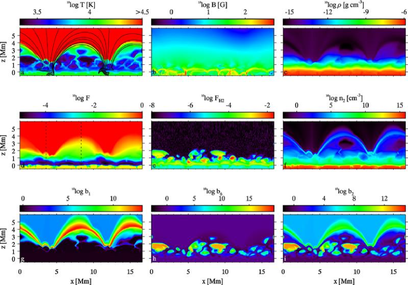
Figure 1: Snapshot cutouts from the simulation, showing various quantities in a vertical plane after 8.5 minutes of solar-time evolution. Panel a: gas temperature, with magnetic field lines that extend into the corona overplotted in black; b: magnetic field strength; c: mass density d: non-equilibrium ionization degree of hydrogen; e: fraction of hydrogen atoms in the form of H₂ molecules; f: hydrogen $n\!=\!2$ level population; g: departure coefficient for the hydrogen $n\!=\!1$ level population; h: departure coefficient for the hydrogen $n\!=\!6$ level population; i: departure coefficient for the hydrogen $n\!=\!2$ level population. The columns used in Figs. 2 and 3 are indicated by dotted lines in panel d.

3 Results

Figure 1 shows a snapshot of the simulation. Panel a displays the temperature. Some magnetic field lines that extend into the corona have been overplotted. All coronal field lines are rooted in two photospheric magnetic field concentrations at $x\!=\!4$ and $x\!=\!11$ Mm. Henceforth we refer to these concentrations as magnetic elements and to the areas between them as internetwork.

The areas without field lines are not field free, as can be seen in panel b which shows the magnitude of the magnetic field strength. The temperature panel displays granulation at $z\!=\!0$ Mm, a shock-ridden chromosphere up to $2-4$ Mm height, and a hot corona reaching peak temperatures of $10^{6}$ K. The height and shape of the transition region strongly depend on the magnetic field configuration, with the corona reaching deeper down above the magnetic elements. Panel c shows the mass density. It reaches minimum values in the transition region above internetwork, which consists of extended high-rising arcs (black in the panel).

Panel d shows the non-equilibrium hydrogen ionization degree. It has a minimum between 0 and 0.5 Mm and smoothly increases upward to the completely ionized corona. The chromospheric ionization degree does not follow the local gas temperature. Panel e shows the fraction of hydrogen nuclei bound in H₂ molecules, which peaks in cool chromospheric regions between 0.5 and 2 Mm. The black-purple noise above $z\!=\!2$ Mm is a numerical artifact caused by the single precision output of the code. The code itself uses double precision to avoid such artifacts. Panel f shows the population density of hydrogen in the $n\!=\!2$ level, the lower level of the H $\alpha$ line. It roughly follows the density structure, with the exception of the transition region where it shows a sharp increase at the locations of the arcs of minimum mass density.

Panel g shows the non-LTE population departure coefficient of the ground state of hydrogen $b_{1}$. The ground state population remains close to LTE throughout most of the photosphere and chromosphere, except in strong chromospheric shocks where there is under-ionization compared to LTE. The ground state is strongly overpopulated in the transition region and is in coronal equilibrium in the corona.

Panel h shows the departure coefficient of the hydrogen ion density $b_{6}$. It is much larger than unity in chromospheric cool intershock regions and smaller than unity within chromospheric shocks. This demonstrates that the non-equilibrium ionization degree is higher than in LTE in intershock areas and lower in shocks.

The departure coefficient of the $n\!=\!2$ level in panel i shows the same structure in the photoshere and chromosphere as $b_{6}$ due to the strong coupling of the continuum and the excited neutral levels. In the corona, $b_{2}$ is around $5\times 10^{4}$, its coronal equilibrium value.

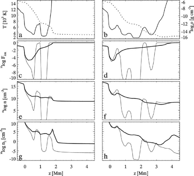
Figure 2: Properties of the simulation along a column in a magnetic element (left-hand column) and in the internetwork (right-hand column). Panels a and b: temperature (solid) and mass density (dashed, right-hand scale); c and d: non-equilibrium (thick) and LTE ionization degree (thin); e and f: non-equilibrium (thick) and LTE proton density (thin); g and h: population of the $n\!=\!2$ level for the non-equilibrium (thick) and LTE (thin) case.

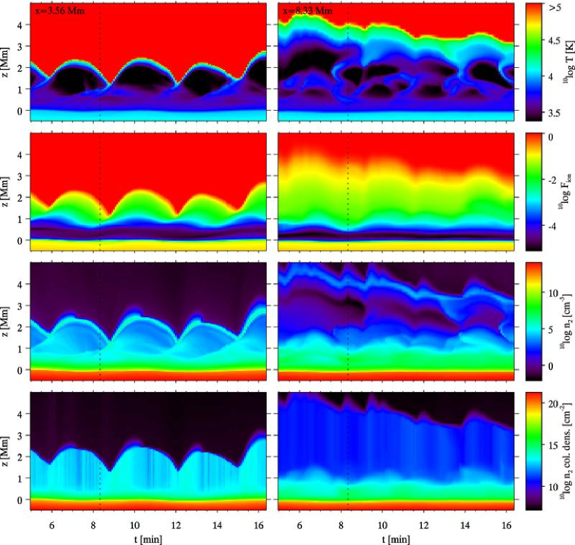
Figure 3: Time slices of the gas temperature (first row), the ionization degree of hydrogen (second row), fraction of hydrogen in the $n\!=\!2$ level (third row), and the $n\!=\!2$ column density (fourth row) in a magnetic element (left-hand column) and in the internetwork (right-hand column). The upper-left magnetic element panel shows dynamic fibrils pushing the corona upward with 3 min periodicity. The upper-right internetwork panel shows rather unstructured shocks and a slowly varying height of the transition region. The snapshot used in Fig. 1 and 2 is indicated by a black dotted line.

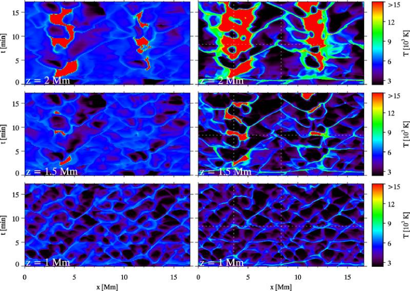
Figure 4: Time slices of the gas temperature at 2, 1.5 and 1 Mm height (top to bottom). Left-hand column: simulation with LTE ionization; right-hand column: with non-equilibrium ionization. Both simulations were started with the same snapshot at $t\!=\!0$ min. The intermittently present red patches are caused by the corona, whose lower boundary is moved up and down by shocks traveling upward above the magnetic elements. The snapshot used in Fig. 1 is indicated with the horizontal dotted line; the columns used in Figs. 2 and 3 with vertical dotted lines.

Figure 2 shows the behavior of atomic hydrogen along the two columns marked in Fig 1. These were selected to sample a magnetic element (left-hand column) and quiet internetwork (right-hand column). Panels a and b show the temperature and mass density. The corona starts much lower above the magnetic element than above the internetwork. Panel a shows a strong shock at 1 Mm which will become a dynamic fibril when it reaches the corona, pushing it upward. In contrast, internetwork panel b shows no strong shocks. The density at the transition region is much lower in this case.

Panels c and d show the non-equilibrium degree of ionization of hydrogen as thick curves. It reaches a minimum of $10^{-5}$ at around 0.5 Mm and increases smoothly towards complete ionization in the corona. The corresponding LTE ionization, obtained from the simulation temperature and electron density stratifications with the Saha-Boltzmann equations, is shown as a thin curve. The dramatic differences between the curves demonstrate the failure of instantaneous LTE ionization in the chromosphere and transition region. In the non-equilibrium case, the slowness of ionization and recombination prevents total ionization in the shocks and full recombination in their wakes, producing far smoother ionization behavior with time than LTE would predict (see Carlsson & Stein 2002; Leenaarts & Wedemeyer-Böhm 2006). Note that the LTE curves reach complete ionization in the transition region at slightly lower heights than the non-equilibrium ionization curves. Since hydrogen becomes the dominant electron provider already at $10^{-4}$ ionization, the electron density equals the proton density except in the temperature minimum.

Panels e and f show the non-equilibrium (thick) and LTE (thin) proton densities. Since hydrogen becomes the dominant electron provider already at $10^{-4}$ ionization, the electron density equals the proton density except in the ionization minimum around 0.5 Mm (panels c and d).

Panels g and h show the population density of the $n\!=\!2$ level of hydrogen $n_{2}$ (thick: non-equilibrium; thin: LTE). It shows the same trend as the proton population, because all excited hydrogen levels are strongly coupled to the proton population reservoir. Thus, the small temporal variation of the ionization is followed by the $n\!=\!2$ population, and, therefore, the H $\alpha$ opacity. In particular, the peaks in $n_{2}$ in the transition region in both panels, at $z\!=\!1.8$ Mm and $z\!=\!4.2$ Mm, respectively, provide significant H $\alpha$ visibility.

Figure 3 shows the temporal evolution of the temperature in a magnetic element and in the internetwork. The magnetic element acts as a wave guide, in which shocks travel upward with a period of three minutes. When they reach the corona they push it upward. With time, these motions produce characteristic parabolic height variation. The same behavior is observed in so-called H $\alpha$ dynamic fibrils. The recent papers by Hansteen et al. (2006) and De Pontieu et al. (2007) show that H $\alpha$ dynamic fibrils are the observational signature of such magneto-acoustic shocks. Notice that the material in the wake of the shocks can be as cool as 2,400 K.

The internetwork temperature is less structured. A movie of the gas temperature (available in the online material for this article) shows that the internetwork chromosphere is pervaded by shocks which originate in the photosphere but often travel sideways, away from the magnetic elements, and sometimes even downward. The transition region is located higher than above a magnetic element and exhibits relatively small and irregular temporal variations in height.

The second row shows the ionization degree of hydrogen. It is rather constant in time in the chromosphere. Above 1 Mm height, it stays at about 1% ionization, both in the magnetic element and the internetwork. The transition to coronal temperatures is smoother in the internetwork and the increase in ionization is correspondingly smoother. The third row displays the population of hydrogen in the $n\!=\!2$ level $n_{2}$. It is very low in the almost completely ionized corona. The transition region shows a local maximum, which is persistent in time. The $n\!=\!2$ population is higher in the transition region of the magnetic element than in the internetwork. The width of the transition region maximum in the upward phase of the dynamic fibrils decreases suddenly when the fibril descends again.

The fourth row displays the column density of $n_{2}$, which is proportional to the vertical optical depth in the H $\alpha$ line. In the internetwork, the column density starts to increase higher in the atmosphere than in the magnetic elements, because the chromosphere extends to larger heights in the internetwork. However, the column density at the top of the dynamic fibrils (the top of the light blue bulges) is $10^{13}$ cm^-2, two orders of magnitude larger than the internetwork column density at equal height. The same column density in the internetwork is reached at a height of 0.8 Mm.

3.1 Comparison with companion LTE simulation

Figure 4 presents a comparison between the simulation with non-equilibrium hydrogen ionization and a simulation with the old code which employs LTE ionization. Both simulations were started at $t\!=\!0$ min from the same relaxed snapshot computed with LTE ionization.

The bottom panels of 4 show that at height $z\!=\!1$ Mm the different treatments of ionization produce only a slight difference in temperature variation. The wave pattern is almost identical, but with non-equilibrium ionization the fluctuations are larger. At larger heights, the differences between the simulations are large (upper two rows). The shock patterns (thin hot threads) differ markedly. The shock temperatures are much larger in the non-equilibrium simulation. They typically are 10,000 K and sometimes reach 13,000 K, whereas the LTE shock temperatures do not exceed 8,000 K. These high temperatures are due to the comparative lack of ionization. Because the internal energy of the gas is not stored as hydrogen ionization energy, it remains as kinetic energy of the gas particles, raising the temperature (Carlsson & Stein 1992).

The temperatures also differ greatly in the cool intershock regions. In LTE, they are between 3,000 and 5,000 K whereas the non-equilibrium simulation reaches intershock temperatures of about 2,500 K. These low values result from the reverse process: over-ionization compared with LTE. More energy remains stored as ionization energy, leaving less kinetic energy for the gas particles.

4 Discussion & Conclusions

4.1 Limitations of the simulation

Our implementation of non-equilibrium hydrogen ionization has various limitations.

First, the assumption that all Lyman transitions are in detailed balance is justified up to the transition region (Sollum 1999). However, the transition region is optically thin in most Lyman features, requiring detailed radiative transfer modeling to evaluate their influence on the hydrogen populations.

Second, the multi-group radiative transfer within the simulation, which sets the radiative cooling and heating, employs LTE ionization. For given internal energy and mass density, the radiative transfer uses the group-mean opacity, scattering probability and Planck function based on the corresponding LTE (or coronal equilibrium) temperature and electron density. The radiative cooling in the chromosphere and transition region, where deviations from equilibrium are largest, is thus inconsistent with the non-equilibrium temperature and electron density as computed in the simulation.

Third, the cool parts of the simulation chromosphere often reach the limiting temperature of 2,400 K allowed in the simulation. It is not clear how low the actual chromospheric minima may reach because radiative heating in the hydrogen continua and other strong spectral features is not taken into account in the simulation, only their radiative cooling.

4.2 Discussion

From the analysis of our simulation we obtain the following picture. The internetwork chromosphere is irregularly pervaded by shocks. The temperature is typically 10,000 K in shocks and can be lower than 2,500 K in cool intershock areas. The transition region is arc-shaped, with the arc footpoints situated above the magnetic elements, and reaches a maximum height of 4 Mm. The chromosphere above magnetic elements shows upward propagating shocks at about 3 minute periodicity, which push the corona upward from 1.5 Mm to 3 Mm height.

The chromospheric hydrogen ionization degree increases smoothly from $10^{-5}$ at 0.5 Mm to complete ionization in the corona and does not respond to temperature changes because of the slow recombination behind shocks. The hydrogen $n\!=\!2$ population in the chromosphere is coupled to the proton population and, as a consequence, varies only weakly with time too. The $n\!=\!2$ population in dynamic fibrils above the magnetic elements is higher than in the internetwork chromosphere. The $n\!=\!2$ column density, a measure of the optical depth of the H $\alpha$ line, is two orders of magnitude larger in dynamic fibrils than at equal height in the internetwork. The same column density as at the top of the fibrils is only reached at a smaller height, about 0.8 Mm, in the internetwork.

In the observations of Hansteen et al. (2006) and De Pontieu et al. (2007) dynamic fibrils appear as dark “fingers” extending and retracting on top of a brighter background. They seem to be optically thick. Combining this observational appearance with the results of our simulation suggests that dynamic fibrils are optically thick in the H $\alpha$ line core, whereas optical depth unity is reached far deeper in the internetwork atmosphere (equal column density in the lower panels of Fig. 3) so that the internetwork chromosphere adjacent to dynamic fibrils is optically thin. This explains that dynamic fibrils are observable along a slanted line of sight through the internetwork chromosphere. We also suggest that their low temperature combined with the effects of NLTE resonance scattering produces their low emergent intensity. The bright background is formed much deeper in the internetwork, where the higher temperature leads to higher emergent intensity. In summary, slow recombination and strong coupling of the $n\!=\!2$ population to the ion population makes these fibrils opaque and therefore visible even when they are cool, regardless of the large $n\!=\!2$ excitation energy. H $\alpha$ interpretation assuming a static atmosphere with instantaneous ionization and recombination, as frequently done in cloud modeling and inversions based on cloud modeling, is likely to be erroneous for such dynamic structures. Obviously, detailed radiative transfer computation based on time-dependent simulation with non-equilibrium ionization as done here is needed to properly assess H $\alpha$ formation in dynamic fibrils.

4.3 Conclusions

We have presented an algorithm to compute non-equilibrium hydrogen ionization with back-coupling to the equation of state in multidimensional radiation MHD simulations of the solar atmosphere. We performed a 2D simulation from the convection zone to the corona that employed this algorithm. From its analysis and comparison with a companion LTE simulation we conclude the following:

• Inclusion of non-equilibrium hydrogen ionization is essential in simulations of the solar atmosphere because the resulting temperature structure and hydrogen populations differ dramatically from their LTE values.

• The degree of ionization of hydrogen in the chromosphere does not follow the local temperature, as described already by Carlsson & Stein (2002) and Leenaarts & Wedemeyer-Böhm (2006). Hydrogen is partially ionized in shocks but does not recombine in the cool shock wakes, owing to the slow recombination rate at low temperature (Figs. 1, 2, and 3).

• Non-equilibrium hydrogen ionization causes more profound temperature variations in the chromosphere than would occur if LTE were valid (Fig. 4). The shock temperatures are higher and the intershock temperatures are lower, caused by the insensitivity of the hydrogen ionization degree to variations of the state parameters of the gas.

• The population of the hydrogen $n\!=\!2$ level in the chromosphere is strongly coupled to the ion population. It therefore behaves approximately as the latter. Its value is set by the high shock temperatures and subsequently remains high in the cool aftershock phases (Fig. 2). This is quite contrary to the LTE prediction.

• The simulation shows large differences in temperature structure and hydrogen level populations between magnetic elements and internetwork (Figs. 2 and 3).

• The H $\alpha$ line opacity is proportional to the $n\!=\!2$ level population; the H $\alpha$ optical depth scales with the $n\!=\!2$ column density. Both are appreciably larger in dynamic fibrils than in the internetwork chromosphere at equal height (Fig. 3). We suggest that dynamic fibrils are optically thick in H $\alpha$ and that their low temperature combined with scattering make them appear dark against the deeper-formed bright internetwork background.

The next step is to compute H $\alpha$ in detail from this simulation.

Appendix A The equations and their derivatives

The solution scheme requires partial derivatives with respect to the independent variables. The formulation is similar to the RADYN code of Carlsson & Stein (1992) but since no detailed specification has been published so far, we supply the complete derivative list here.

The present code solves the equations of chemical equilibrium, charge, energy and hydrogen nucleus conservation together with the rate equations or with the Saha-Boltzmann equilibrium equations. These equations depend on the gas temperature $T$, the electron density $n_{\rm e}$, the hydrogen population densities $n_{i}$, where $n_{1}$ is the ground state, $n_{2-5}$ the four excited states and $n_{6}$ the ionized hydrogen (proton) density, and the molecular hydrogen density $n_{\mathrm{H2}}$. These are ten equations and nine unknowns. We use only five of the six rate equations and eliminate the molecular hydrogen density, reducing the number of equations and variables to eight. The equations are labeled $F_{i}$ with $i=1,\ldots,8$.

The physical constants have their usual meaning: $h$, $k$, $c$, $e$ and $m_{{\rm e}}$ are Planck’s constant, Boltzmann’s constant, the velocity of light, the electron charge and the electron mass.

As the mass density of the gas is known, the total number of hydrogen nuclei, whether in the form of H, H₂ or bare protons is known and given by

$$n_{\mathrm{H}}^{\mathrm{tot}}\!=\!\rho\,n_{\mathrm{H\,per\,g}}$$ (7)

where $n_{\mathrm{H\,per\,g}}$ is the number of hydrogen nuclei per gram solar gas. We denote the number density of nuclei of elements other than hydrogen as $n_{\mathrm{noH}}=n_{\mathrm{nuclei\,per\,H}}\,n_{\mathrm{H}}^{\mathrm{tot}}$, where $n_{\mathrm{nuclei\,per\,H}}$ is the number of nuclei from elements other than hydrogen per hydrogen nucleus. The number of electrons due to elements other than hydrogen per hydrogen nucleus is $n_{\rm e}^{\mathrm{noH}}$. The internal energy of elements other than hydrogen per hydrogen nucleus is $e_{\mathrm{noH}}$. These quantities and their derivatives are determined numerically from tables as function of $T$ and $n_{\rm e}$. The molecular hydrogen density is $n_{\mathrm{H2}}$ and the internal energy of H₂ per molecule is $e_{\mathrm{H2}}$. The latter is computed using polynomial approximations by Vardya (1965)

Chemical equilibrium.

The equation of chemical equilibrium between neutral atomic hydrogen and molecular hydrogen is given by

$$n_{\mathrm{H2}}=\frac{\left(\sum_{i=1}^{5}n_{i}\right)^{2}}{K},$$ (8)

where $K$ is the chemical equilibrium constant whose value and its temperature derivative are given by polynomial approximations as function of $T$ by Tsuji (1973). The molecular hydrogen density depends on $T$ and $n_{i}$ ($i=1,\ldots,5$). The derivatives are

$$\frac{\partial n_{\mathrm{H2}}}{\partial T} = -\left(\frac{\sum_{i=1}^{5}n_{i}}{K}\right)^{2}\frac{\partial K}{\partial T},$$ (9)

$$\frac{\partial n_{\mathrm{H2}}}{\partial n_{i}} = \frac{2\left(\sum_{i=1}^{5}n_{i}\right)}{K}.$$ (10)

Charge conservation.

The electron density is given by

$$n_{\rm e}=n_{6}+n_{\mathrm{H}}^{\mathrm{tot}}n_{\rm e}^{\mathrm{noH}},$$ (11)

which we rewrite in a form suitable for Newton-Raphson iteration:

$$F_{1}=1-\frac{1}{n_{\rm e}}\left(n_{6}+n_{\mathrm{H}}^{\mathrm{tot}}n_{\rm e}^{\mathrm{noH}}\right)=0.$$ (12)

The functional $F_{1}$ depends on $n_{\rm e}$, $n_{6}$ and $T$. The partial derivatives are

$$\frac{\partial F_{1}}{\partial n_{\rm e}} = \frac{n_{6}+n_{\mathrm{H}}^{\mathrm{tot}}n_{\rm e}^{\mathrm{noH}}}{n_{\rm e}^{2}}-\frac{n_{\mathrm{H}}^{\mathrm{tot}}}{n_{\rm e}}\frac{\partial n_{\rm e}^{\mathrm{noH}}}{\partial n_{\rm e}},$$ (13)

$$\frac{\partial F_{1}}{\partial n_{6}} = -\frac{1}{n_{\rm e}},$$ (14)

$$\frac{\partial F_{1}}{\partial T} = -\frac{n_{\mathrm{H}}^{\mathrm{tot}}}{n_{\rm e}}\frac{\partial n_{\rm e}^{\mathrm{noH}}}{\partial T}.$$ (15)

Internal energy.

The second functional specifies the distribution of the internal energy $e_{\mathrm{i}}$ over the various contributions:

$$F_{2} = 1-\frac{1}{e_{\mathrm{i}}}\left(\frac{3kT}{2}\left[n_{\rm e}+n_{\mathrm{noH}}+n_{\mathrm{H2}}+\sum_{i=1}^{6}n_{i}\right]\right.$$ (16)

$$+\left.n_{\mathrm{H}}^{\mathrm{tot}}\,e_{\mathrm{noH}}+n_{\mathrm{H2}}\,e_{\mathrm{H2}}+\sum_{i=1}^{6}n_{i}\,\chi_{i}\right)=0,$$

with $\chi_{i}$ the energy of hydrogen level $i$. This functional depends on $n_{\rm e}$, $n_{i}$ and $T$. The partial derivatives are

$$\frac{\partial F_{2}}{\partial n_{\rm e}} = -\frac{1}{e_{\mathrm{i}}}\left(\frac{3kT}{2}+n_{\mathrm{H}}^{\mathrm{tot}}\frac{\partial e_{\mathrm{noH}}}{\partial n_{\rm e}}\right),$$ (17)

$$\frac{\partial F_{2}}{\partial n_{i}} = -\frac{1}{e_{\mathrm{i}}}\left(\frac{3kT}{2}\left[\frac{\partial n_{\mathrm{H2}}}{\partial n_{i}}+1\right]+e_{\mathrm{H2}}\frac{\partial n_{\mathrm{H2}}}{\partial n_{i}}+\chi_{i}\right),$$ (18)

$$\frac{\partial F_{2}}{\partial T} = -\frac{1}{e_{\mathrm{i}}}\left(\frac{3k}{2}\left[n_{\rm e}+n_{\mathrm{noH}}+n_{\mathrm{H2}}+T\frac{\partial n_{\mathrm{H2}}}{\partial T}+\sum_{i=1}^{6}n_{i}\right]\right.$$ (19)

$$\left.+n_{\mathrm{H}}^{\mathrm{tot}}\frac{\partial e_{\mathrm{noH}}}{\partial T}+n_{\mathrm{H2}}\frac{\partial e_{\mathrm{H2}}}{\partial T}+e_{\mathrm{H2}}\frac{\partial n_{\mathrm{H2}}}{\partial T}\right).$$

Particle conservation.

The conservation of the total number of hydrogen nuclei $n_{\mathrm{H}}^{\mathrm{tot}}$ is given by:

$$F_{3}=1-\frac{1}{n_{\mathrm{H}}^{\mathrm{tot}}}\left(\sum_{i=1}^{6}n_{i}-2n_{\mathrm{H2}}\right)=0.$$ (20)

This functional depends on $n_{i}$ and $T$. The partial derivatives are:

$$\frac{\partial F_{3}}{\partial n_{i}} = -\frac{1}{n_{\mathrm{H}}^{\mathrm{tot}}}\left(1+2\frac{\partial n_{\mathrm{H2}}}{\partial n_{i}}\right),i=1,\ldots,5,$$ (21)

$$\frac{\partial F_{3}}{\partial n_{6}} = -\frac{1}{n_{\mathrm{H}}^{\mathrm{tot}}},$$ (22)

$$\frac{\partial F_{3}}{\partial T} = -\frac{2}{n_{\mathrm{H}}^{\mathrm{tot}}}\frac{\partial n_{\mathrm{H2}}}{\partial T}.$$ (23)

LTE populations.

LTE is imposed to start up a new computation and at the lower boundary. The LTE hydrogen populations then obey the Saha-Boltzmann equations ($i=1,\ldots,5$)

$$F_{3+i}=1-\frac{1}{n_{\rm e}}\frac{n_{i}}{n_{6}}\frac{2g_{6}}{g_{i}}\left(\frac{2\pi m_{{\rm e}}kT}{h^{2}}\right)^{3/2}{\rm e}^{-(\chi_{6}-\chi_{i})/kT}=0,$$ (24)

where $g_{i}$ is the statistical weight of level $i$. These equations depend on $n_{6}$, $n_{i}$, $n_{\rm e}$ and $T$. Defining

$$K_{i}=\frac{1}{n_{\rm e}}\frac{n_{i}}{n_{6}}\frac{2g_{6}}{g_{i}}\left(\frac{2\pi m_{{\rm e}}kT}{h^{2}}\right)^{3/2}{\rm e}^{-(\chi_{6}-\chi_{i})/kT},$$ (25)

the partial derivatives are given by

$$\frac{\partial F_{3+i}}{\partial n_{6}} = \frac{K_{i}}{n_{6}},$$ (26)

$$\frac{\partial F_{3+i}}{\partial n_{i}} = -\frac{K_{i}}{n_{i}},$$ (27)

$$\frac{\partial F_{3+i}}{\partial n_{\rm e}} = \frac{K_{i}}{n_{\rm e}},$$ (28)

$$\frac{\partial F_{3+i}}{\partial T} = -K_{i}\left(\ \frac{\chi_{6}-\chi_{i}}{kT^{2}}+\frac{3}{2T}\right).$$ (29)

Rate equations.

Outside LTE, the change of the hydrogen populations $n_{1}\ldots n_{6}$ over a timestep $\Delta t$ can be expressed as

$$n_{i}(t_{0}+\Delta t)-n_{i}(t_{0}) = \int_{t_{0}}^{t_{0}+\Delta t}\sum_{j,j\neq i}^{6}n_{j}\left(R_{ji}+C_{ji}\right)$$ (30)

$$-n_{i}\sum_{j,j\neq i}^{6}\left(R_{ij}+C_{ij}\right)\,{\rm d}t,$$

with $R_{ij}$ and $C_{ij}$ the radiative and collisional rate coefficients from level $i$ to level $j$. Defining

$$P_{ij} = R_{ij}+C_{ij},$$ (31)

$$P_{ii} = -\sum_{j,j\neq i}^{6}\left(R_{ij}+C_{ij}\right)$$ (32)

and writing $n_{i}=n_{i}\,(t_{0}+\Delta t)$ and $n_{i}^{t_{0}}=n_{i}\,(t_{0})$ yields the discretized, implicit form of Eq. 30

$$F_{3+i}=\frac{n_{i}}{n_{i}^{t_{0}}}-\frac{\Delta t}{n_{i}^{t_{0}}}\left(\sum_{j=1}^{6}n_{j}P_{ji}\right)-1=0.$$ (33)

The equations are dependent on $n_{i}$, $n_{j}$ ($j\neq i$), $n_{\rm e}$ and $T$. The partial derivatives are

$$\frac{\partial F_{3+i}}{\partial n_{i}} = \frac{1-\Delta t\,P_{ii}}{n_{i}^{t_{0}}},$$ (34)

$$\frac{\partial F_{3+i}}{\partial n_{j}} = -\frac{\Delta t\,P_{ji}}{n_{i}^{t_{0}}},$$ (35)

$$\frac{\partial F_{3+i}}{\partial n_{\rm e}} = -\frac{\Delta t}{n_{i}^{t_{0}}}\left(\sum_{j=1}^{6}n_{j}\frac{\partial P_{ji}}{\partial n_{\rm e}}\right),$$ (36)

$$\frac{\partial F_{3+i}}{\partial T} = -\frac{\Delta t}{n_{i}^{t_{0}}}\left(\sum_{j=1}^{6}n_{j}\frac{\partial P_{ji}}{\partial T}\right).$$ (37)

Only five of the six equations 30 are used to avoid overspecification through ignoring the one with the largest value of $n_{i}^{t_{0}}$.

LTE population ratios.

Evaluation of the rate coefficients involving the continuum level $n_{6}$ often involve the LTE population ratio $n^{*}_{i}/n^{*}_{6}$ ($i=1,\ldots,5$) given by

$$\frac{n^{*}_{i}}{n^{*}_{6}}=n_{\rm e}\frac{g_{i}}{2g_{6}}\left(\frac{2\pi m_{{\rm e}}kT}{h^{2}}\right)^{-3/2}{\rm e}^{(\chi_{6}-\chi_{i})/kT},$$ (38)

with the derivatives

$$\frac{\partial}{\partial T}\left(\frac{n^{*}_{6}}{n^{*}_{i}}\right) = -\left(\ \frac{\chi_{6}-\chi_{i}}{kT^{2}}+\frac{3}{2T}\right)\frac{n^{*}_{i}}{n^{*}_{6}},$$ (39)

$$\frac{\partial}{\partial n_{\rm e}}\left(\frac{n^{*}_{i}}{n^{*}_{6}}\right) = \frac{1}{n_{\rm e}}\frac{n^{*}_{i}}{n^{*}_{6}}.$$ (40)

Collisional rate coefficients.

The expressions for the collisional rate coefficients contain temperature-dependent coefficients $C_{\mathrm{exc}}$ and $C_{\mathrm{ion}}$ for excitation and ionization. Their values and derivatives are determined from a table based on Johnson (1972).

The collisional rate coefficients for bound-bound transitions are, with $j>i$ and $C_{ij}$ the upward rate coefficient:

$$C_{ji} = \frac{g_{i}}{g_{j}}n_{\rm e}C_{\mathrm{exc}}\sqrt{T},$$ (41)

$$C_{ij} = \frac{n^{*}_{j}}{n^{*}_{i}}C_{ji}=n_{\rm e}C_{\mathrm{exc}}\sqrt{T}\,{\rm e}^{-(\chi_{j}-\chi_{i})/kT},$$ (42)

with derivatives

$$\frac{\partial C_{ji}}{\partial n_{\rm e}} = \frac{C_{ji}}{n_{\rm e}},$$ (43)

$$\frac{\partial C_{ji}}{\partial T} = \frac{g_{i}}{g_{j}}n_{\rm e}\sqrt{T}\left(\frac{\partial C_{\mathrm{exc}}}{\partial T}+\frac{C_{\mathrm{exc}}}{2T}\right),$$ (44)

$$\frac{\partial C_{ij}}{\partial n_{\rm e}} = \frac{C_{ij}}{n_{\rm e}},$$ (45)

$$\frac{\partial C_{ij}}{\partial T} = n_{\rm e}\sqrt{T}{\rm e}^{-(\chi_{j}-\chi_{i})/kT}\left(\frac{\partial C_{\mathrm{exc}}}{\partial T}+C_{\mathrm{exc}}\left[\frac{\chi_{j}-\chi_{i}}{kT^{2}}+\frac{1}{2T}\right]\right)$$ (46)

For bound-free transitions the collision rate coefficients are, with $C_{i6}$ the upward rate coefficient:

$$C_{i6} = n_{\rm e}C_{\mathrm{ion}}(T)\sqrt{T}{\rm e}^{-(\chi_{6}-\chi_{i})/kT},$$ (47)

$$C_{6i} = \frac{n^{*}_{i}}{n^{*}_{6}}C_{i6},$$ (48)

with derivatives

$$\frac{\partial C_{i6}}{\partial n_{\rm e}} = \frac{C_{i6}}{n_{\rm e}},$$ (49)

$$\frac{\partial C_{i6}}{\partial T} = n_{\rm e}\sqrt{T}{\rm e}^{-(\chi_{6}-\chi_{i})/kT}\left(\frac{\partial C_{\mathrm{ion}}}{\partial T}+C_{\mathrm{ion}}\left[\frac{\chi_{6}-\chi_{i}}{kT^{2}}+\frac{1}{2T}\right]\right)$$ (50)

$$\frac{\partial C_{6i}}{\partial n_{\rm e}} = 2\frac{C_{6i}}{n_{\rm e}},$$ (51)

$$\frac{\partial C_{6i}}{\partial T} = \left(\frac{\partial C_{i6}}{\partial T}-C_{6i}\left[\frac{3}{2T}+\frac{\chi_{6}-\chi_{i}}{kT^{2}}\right]\right)\frac{n^{*}_{6}}{n^{*}_{i}}.$$ (52)

Radiative rate coefficients.

The derivation of the radiative rate coefficients can be found in Sollum (1999). The rate coefficients for bound-bound transitions are, with $j>i$ and $R_{ij}$ the upward rate coefficient:

$$R_{ij} = \frac{4\pi^{2}e^{2}}{h\nu_{0}m_{{\rm e}}c}f_{{\rm l}{\rm u}}\frac{2h\nu_{0}^{3}}{c^{2}}\frac{1}{{\rm e}^{h\nu_{0}/kT_{{\rm r}{\rm a}{\rm d}}}-1},$$ (53)

$$R_{ji} = \frac{g_{i}}{g_{j}}\frac{4\pi^{2}e^{2}}{h\nu_{0}m_{{\rm e}}c}f_{{\rm l}{\rm u}}\frac{2h\nu_{0}^{3}}{c^{2}}\frac{1}{1-{\rm e}^{-h\nu_{0}/kT_{{\rm r}{\rm a}{\rm d}}}},$$ (54)

where $f_{{\rm l}{\rm u}}$, $\nu_{0}$ and $T_{{\rm r}{\rm a}{\rm d}}$ are the oscillator strength, the line center frequency and the prescribed radiation temperature. In areas where $T_{{\rm r}{\rm a}{\rm d}}\!=\!T$, i.e., deep in the atmosphere, the temperature derivatives are:

$$\frac{\partial R_{ij}}{\partial T} = \frac{8\pi^{2}e^{2}h\nu_{0}^{3}}{m_{{\rm e}}c^{3}kT^{2}}f_{ij}\frac{{\rm e}^{-h\nu_{0}/kT}}{(1-{\rm e}^{-h\nu_{0}/kT})^{2}},$$ (55)

$$\frac{\partial R_{ji}}{\partial T} = \frac{g_{i}}{g_{j}}\frac{8\pi^{2}e^{2}h\nu_{0}^{3}}{m_{{\rm e}}c^{3}kT^{2}}f_{ij}\frac{{\rm e}^{h\nu_{0}/kT}}{({\rm e}^{h\nu_{0}/kT}-1)^{2}},$$ (56)

In areas where $T_{{\rm r}{\rm a}{\rm d}}\neq T$, but constant, the temperature derivatives are zero.

The upward radiative rate coefficient for bound-free transitions is:

$$R_{i6}=\frac{8\pi}{c^{2}}\alpha_{0}\nu_{0}^{3}\sum_{n=1}^{\infty}E_{1}\left(n\frac{h\nu_{0}}{kT_{{\rm r}{\rm a}{\rm d}}}\right),$$ (57)

where $\alpha_{0}$ is the radiative absorption cross section at the ionization edge frequency $\nu_{0}$ and $E_{1}(x)$ the first exponential integral with argument $x$. Its temperature derivative is:

$$\frac{\partial R_{i6}}{\partial T} = \frac{8\pi}{c^{2}}\alpha_{0}\nu_{0}^{3}\frac{1}{T}\frac{1}{{\rm e}^{h\nu_{0}/kT}-1}\ \mathrm{where}\ T_{\mathrm{rad}}\!=\!T,$$ (58)

$$\frac{\partial R_{i6}}{\partial T} = 0\ \mathrm{where}\ T_{\mathrm{rad}}\neq T.$$ (59)

The downward bound-free radiative rate coefficient is:

$$R_{6i}=\frac{8\pi}{c^{2}}\alpha_{0}\nu_{0}^{3}\frac{n^{*}_{i}}{n^{*}_{6}}\sum_{n=1}^{\infty}E_{1}\left(\left[n\frac{T}{T_{{\rm r}{\rm a}{\rm d}}}+1\right]\frac{h\nu_{0}}{kT}\right),$$ (60)

The derivatives are:

$$\frac{\partial R_{6i}}{\partial n_{\rm e}} = \frac{R_{6i}}{n_{\rm e}},$$ (61)

$$\frac{\partial R_{6i}}{\partial T} = \frac{\partial R_{i6}}{\partial T}\frac{n^{*}_{i}}{n^{*}_{6}}-R_{6i}\left(\frac{3}{2T}+\frac{h\nu_{0}}{kT^{2}}\right)\ \mathrm{where}\ T_{\mathrm{rad}}\!=\!T,$$ (62)

$$\frac{\partial R_{6i}}{\partial T} = \frac{8\pi}{c^{2}}\alpha_{0}\nu_{0}^{3}\left(\sum_{n=1}^{\infty}\frac{\mathrm{exp}\left(-n\frac{h\nu_{0}}{kT_{{\rm r}{\rm a}{\rm d}}}-\frac{h\nu_{0}}{kT}\right)}{nT+T_{{\rm r}{\rm a}{\rm d}}}\frac{T_{{\rm r}{\rm a}{\rm d}}}{T}\right)\frac{n^{*}_{i}}{n^{*}_{6}}$$ (63)

$$-R_{6i}\left(\frac{3}{2T}+\frac{h\nu_{0}}{kT^{2}}\right)\ \mathrm{where}\ T_{\mathrm{rad}}\neq T.$$