Improved transfer matrix method without numerical instability

Abstract

A new improved transfer matrix method (TMM) is presented. It is shown that the method not only overcomes the numerical instability found in the original TMM, but also greatly improves the scalability of computation. The new improved TMM has no extra cost of computing time as the length of homogeneous scattering region becomes large. The comparison between the scattering matrix method(SMM) and our new TMM is given. It clearly shows that our new method is much faster than SMM.

Transfer matrix method (TMM) has been a useful approach for studying the physical properties. There have been many publications on application of the TMM, such as studies of Ising model Shultz ; Morgenstern[1979] ; Morgenstern[1980] ; Cheung[1983] , quantum spin Suzuki[1985] , electronic transport Sautet[1988] ; Wan[1998] , and electronic state in quasi-periodic and aperiodic chains Tao[1994] ; Huang[1998] . TMM is also widely applied in studying the propagation of electric-magnetic wave waveguide , elastic wave stiff and light wave Light in multi-layer systems.

Original TMM(OTMM) can be efficiently used for the studies of periodic system, one boundary problem between two homogeneous media and the scattering problem of a small region sandwiched by two leads. However, OTMM has a fundamental shortcoming due to its numerical instability when the number of transfer steps is beyond a critical value. This has been a major limitation to the application of OTMM. Some approaches have been developed to calculate the transport through a longer scattering area such as scattering matrix method (SMM) Pendry[94] ; Pendry[other1] ; Pendry[other2] , extended transfer-matrix technique (ETMT)Wan[1998] and Green’s function approach(GFA)GFA . In SMM, the middle scattering region is cut into some smaller sections, then the scattering matrices of these sections are found by means of TMM and combined together to get total scattering matrix(SM) recursively. In ETMT, they used a technique to cancel the increasing modes step by step for each slice to avoid the numerical instability. Although the numerical instability in SMM and ETMT does not exist anymore, CPU time cost grows linearly when the length of middle scattering region increases. GFA too. Based on a continuous Schrödinger equation in electron wave guide without spin-orbit coupling(SOC)HuaWu and with SOCYaoYang , the stable solution of transport were also achieved. However, there are infinite number of evanescent modes that pose tremendous numerical difficulty, and the approximation of limit number of evanescent wave must be done. But in some case, the contribution of evanescent wave is significant, even more in the presence of SOCYaoYang ; LiYang . In this letter, we present a new improved TMM (NITMM) that has overcome such non-physical numerical instability of OTMM. Our study will focus on the discrete version of Schrödinger equation with Rashba SOCRashba[1960] and will find the exact solution of electron transport with and without SOC. Our new method not only gives numerically stable solution at any length of the sample, but also provides high performance in computation. That is, no extra computing costs at increasing length of sample. Meanwhile the simplicity of OTMM is still maintained.

General formulae of TMM. A $2d$ strip with the geometry of a bar sandwiched by two semi-infinite leads is studied. The Hamiltonian of $2d$ electron gas is

$$\hat{H}=\frac{\hat{p}_{x}^{2}+\hat{p}_{y}^{2}}{2m^{\ast}}+V(x,y)+H_{so},$$ (1)

where $V(x,y)$ is the potential including confinement boundary, $H_{so}$ the remainder of the Hamiltonian that may contain spin-orbit coupling. After discretization of the Schrödinger equation $\hat{H}\Psi(x,y)=E\Psi(x,y),$ the strip is replaced by a lattice array with $N$ infinite long chains. The lattice constant is assumed to be $a.$ Wider strip needs larger chain number $N$ to represent. The Schrödinger equation can be transformed into the following transfer matrix (TM) equations:

$$\Phi_{i+1}=T_{i}\Phi_{i},\Phi_{i+m}=(\prod\nolimits_{i=1}^{m}T_{i})\Phi_{i},$$ (2)

where $\Phi_{i}=(\phi_{i,N,\uparrow},\phi_{i-1,N,\uparrow},\phi_{i,N,\downarrow},\phi_{i-1,N,\downarrow},\cdots,\phi_{i,1,\uparrow}$, $\phi_{i-1,1,\uparrow},\phi_{i,1,\downarrow},\phi_{i-1,1,\downarrow})^{t}$. $\Phi_{i}$ is a matrix with dimension $4N\times 1$. The superscript $t$ means transpose of matrix. The element $\phi_{i,j,\sigma}$ in $\Phi_{i}$ is the value of wave function $\Psi(x,y)$ at site $(i,j)$ with spin index $\sigma.$ The lattice indices are $\{(i,j)\mid i\in(-\infty,\infty),j\in(1,N)\}$. The left lead is in the region $i\in(-\infty,-L-1],$ the right lead in $i\in[L+1,\infty)$, and middle bar in $i\in[-L+1,L-1]$. Two interfaces are at $i=-L$ and $i=L$. $T_{i}$ is a $4N\times 4N$ TM between the wave functions $\Phi_{i}$ and $\Phi_{i+1}.$ Two leads can be different or the same, and here we assume they are the same. Further, we assume that the leads and middle bar are homogeneous. Thus we have four different transfer matrices: $T_{l}$ is the TM in two leads, $T_{so}$ in bar, $T_{S_{L}}$ and $T_{S_{R}}$ at left and right interface respectively.

Fixing adjustable parameters like hopping constant $t_{0},$ on-site potential and the energy of electron $E$, we can obtain all elements of four TM matrices $\{T_{l},T_{so},T_{S_{L}},T_{S_{R}}\}.$ It can be verified that the determinants of $T_{l}$ and $T_{so}$ within homogeneous regions are 1. Then two transform matrices $U_{l}$ and $U_{so}$ can be numerically solved to diagonalize $T_{l}$ and $T_{so}$: $D_{l}=U_{l}T_{l}U_{l}^{-1}$ and $D_{so}=U_{so}T_{so}U_{so}^{-1}$. When one knows the matrix $\Phi_{i}$ at an arbitrary site $i,$ in principle, the wave function can be found anywhere by TM equations. We denote $\widetilde{\Phi}_{i}=U_{l}\Phi_{i}\$in leads and $\widetilde{\Phi}_{i}=U_{so}\Phi_{i}$ in middle bar. The TM equations in diagonal representation can be written as

$$\widetilde{\Phi}_{i+1}=\left\{\begin{array}[]{l}D_{l}\widetilde{\Phi}_{i},\ i\in(-\infty,-L-1]\cup[L+1,\infty),\\ D_{so}\widetilde{\Phi}_{i},\ i\in[-L+1,L-1].\end{array}\right.$$ (3)

When the strip has no interface and fully homogenous or only one interface and two sides are homogeneous, it has been shown that the OTMM works well and has no numerical instability. In this letter, we study the strip with two interfaces. In this case, the OTMM will have serious overflow problem if the length of the middle bar between two leads is longer than a critical value.

We denote $D_{so}$ and $D_{l}$ as $D^{(c)},c=so,l.$ The diagonal elements $\lambda_{i}^{(c)}=D_{ii}^{(c)}$ can be classified into two types: $|\lambda_{i}^{(c)}|=1$ and $|\lambda_{i}^{(c)}|\neq 1$ which relate to propagating and evanescent modes respectively. For mode $|\lambda_{i}^{(c)}|=1$, it can be rewritten as $e^{\pm ik_{i}a}$, where $k_{i}(>0)$ is a real number, and $a$ is the lattice constant. $e^{ik_{i}a}$ is called as “right going” wave, and $e^{-ik_{i}a}$ the “left going”.   For mode $|\lambda_{i}^{(c)}|\neq 1$, it can be rewritten as $e^{\pm(\eta_{i}a+i\phi_{i})}$ where $\eta_{i}$ is a positive real number and $\phi_{i}$ the phase. The $e^{\eta_{i}a+i\phi_{i}}$ is a “right growing” or say “left decaying” mode, and $e^{-\eta_{i}a-i\phi_{i}}$ the “right decaying” or “left growing”. Due to $\det T_{i}=\det D^{(c)}=1$ in homogenous region, any modes $e^{\pm ik_{i}a}$ or $e^{\pm(\eta_{i}a+i\phi_{i})}$ must appear in pairs. Then we can always arrange the diagonal elements into the order: $diag\{D^{(c)}\}=\{e^{ik_{1}a},...,e^{ik_{p}a},e^{-\eta_{1}a-i\phi_{1}},\cdots,e^{-\eta_{q}a-i\phi_{q}},e^{-ik_{1}a},...,e^{-ik_{p}a}\newline ,e^{\eta_{1}a+i\phi_{1}},...,e^{\eta_{q}a+i\phi_{q}}\}.$ The first $p+q$ states in $diag\{D\}$ correspond to $p$ right going and $q$ right decaying modes, and second $p+q$ states to $p$ left going and $q$ left decaying modes. At eigen energy $E,$ totally we have $2p$ propagating modes, and $2q$ evanescent modes. $2p+2q=4N$, $N$ is the number of chains. For each energy $E,$ there are $4N$ modes distributed in $2N$ channels corresponding to $2N$ different $|\lambda_{i}|$, where $|\lambda_{1,\cdots p}|=1$ and $|\lambda_{p+1,\cdots 2N}|>1$. If $q$ equals zero, all states are extended. When $p=0,$ no propagating wave can exist in strip. Changing energy $E$ results in changing of the $p$ and $q.$

We assume that a right going electron wave, $e^{ik_{1}x_{i}},$ is injected from the first channel of left lead. In general there should be some reflection waves in all channels in left lead, due to the scattering of interfaces. We denote the reflection waves in $2N$ channels as $\{r_{l}e^{-ik_{l}x_{i}},r_{p+m}e^{\eta_{m}x_{i}+i\phi_{m}}:l=1,2,...,p;m=1,2,...,q\}.$ $\{r_{l,}r_{p+m}\}$ describe the reflection coefficients. The wave function in the left lead is $\widetilde{\Phi}_{i}=(e^{ik_{1}x_{i}},0,...,0,r_{1}e^{-ik_{1}x_{i}},...,r_{p}e^{-ik_{p}x_{i}},r_{p+1}e^{\eta_{1}x_{i}+i\phi_{1}},...,\newline r_{p+q}e^{\eta_{q}x_{i}+i\phi_{q}})^{t}$. We can further set the wave function at position $i=-L$ to be $\widetilde{\Phi}_{-L}=(1,0,...,0,r_{1},r_{2},..,r_{2N})^{t}$. The phases of reflection waves have been absorbed in coefficients $\{r_{i}\}$. We have $\widetilde{\Phi}_{-L}=D_{l}\widetilde{\Phi}_{-L-1}$, $\widetilde{\Phi}_{-L+1}=\widetilde{T}_{S_{L}}\widetilde{\Phi}_{-L}$, $\widetilde{\Phi}_{L}=(D_{so})^{2L-1}\widetilde{T}_{S_{L}}\widetilde{\Phi}_{-L}$, $\widetilde{\Phi}_{L+1}=\widetilde{S}\widetilde{\Phi}_{-L},$where

$$\left\{\begin{array}[]{l}\widetilde{T}_{S_{L}}=U_{so}T_{S_{L}}U_{l}^{-1},\widetilde{T}_{S_{R}}=U_{l}T_{S_{R}}U_{so}^{-1}\\ \widetilde{S}=\widetilde{T}_{S_{R}}(D_{so})^{2L-1}\widetilde{T}_{S_{L}}\end{array}\right.$$ (4)

Then we have $(\widetilde{\Phi}_{L+1})_{\alpha}=\sum_{\beta=1}^{4N}\widetilde{S}_{\alpha,\beta}(\widetilde{\Phi}_{-L})_{\beta}=\widetilde{S}_{\alpha,1}+\sum_{i=1}^{2N}\widetilde{S}_{\alpha,2N+i}r_{i}$, where $\alpha=1,...,4N$. There are no left going waves injected from right lead, so the wave function at $i=L+1$ can be expressed by $\widetilde{\Phi}_{L+1}=(t_{1},t_{2},...,t_{2N},0,..,0)^{t}$, where $\{t_{i}\}$ are the transmission coefficients. Thus we obtain $2N$ equations:

$$(\widetilde{\Phi}_{L+1})_{\alpha}=0,\alpha=2N+1,\cdots,4N.$$ (5)

Define $2N\times 2N$ matrices $W$ and $Y:$ $W_{lm}=\widetilde{S}_{2N+l,2N+m};Y_{l}=-\widetilde{S}_{2N+l,1};l,m=1,2,...,2N$ and the reflection coefficient matrix $R=(r_{1},r_{2},...,r_{2N})^{t}.$ Equation (5) can be rewritten as $WR=Y$. The matrix $R$ can be uniquely obtained through $R=W^{-1}Y.$ Then $2N$ transmission coefficients can be obtained from equations $t_{\alpha}=(\widetilde{\Phi}_{L+1})_{\alpha}$, $\alpha=1,2,...,2N.$ Hence, the wave function at every site in leads and middle bar is obtained. So basically the electron transport though two interfaces and middle bar is completely solved. However, the computation of $W^{-1}$ will encounter numerical overflow problem when $L$ is large. The problem comes from the term $(D_{so})^{2L-1}$ that may have some increasing modes with diagonal elements like $|\lambda_{p+i}|^{2L-1}.$ If the value of $|\lambda_{p+i}|^{2L-1}$ $\gg 1,$ many elements $W_{lm}=\sum_{i=1}^{4N}(\widetilde{T}_{S_{R}})_{2N+l,i}\lambda_{ii}{}^{2L-1}(\widetilde{T}_{S_{L}})_{i,2N+m}$ are of the order of $|\lambda_{p+i}|^{2L-1}.$ Hence the calculation of $W^{-1}$ will meet the numerical overflow with the order of $\left(\lambda_{p+i}{}^{2L-1}\right)^{n},1\ll n\leq 2N$. Therefore, the OTMM can only accurately solve the solution for bar system with smaller length $L$. For example, we have calculated a Rashba SOC system with $N=200$ by means of OTMM. The longest length of bar is around $15$, and numerical instability happens for $2L>15.$ Larger $N$ results more shorter $2L$.

New improved TM method In fact, the physics here must be finite. The solution for $\{r_{i}\}$ should be stable. The numerical overflow is an artifact of the OTMM. Even $|\lambda_{i}|^{2L-1}$ $\gg 1$ for evanescent modes when $2L-1\gg 1,$ the wave function after $2L-1$ steps of the transfer by $\left(D_{so}\right)^{2L-1}$ still should be finite. Thus the values of $(\widetilde{T}_{S_{L}}\widetilde{\Phi}_{-L})_{2N+p+i},i=1,2,...,q,$ corresponding to the increasing modes of $\{|\lambda_{p+i}|>1\}$ must be very small to assure $(\left(D_{so}\right)^{2L-1}\widetilde{T}_{S_{L}}\widetilde{\Phi}_{-L})_{2N+p+i}$ to be finite. That is the physical requirement. Thus we introduce $q$ new auxiliary parameters $\{\zeta_{i}\}$ and assume that

$$(\widetilde{T}_{S_{L}}\widetilde{\Phi}_{-L})_{2N+p+i}=\zeta_{i}e^{-(2L-1)\left(\eta_{i}a+i\phi_{i}\right)},i=1,...,q.$$ (6)

$q$ parameters $\{\zeta_{i}\}$ have to be determined together with $2N$ reflection coefficients $\{r_{i}\}$. The elements in matrix $\widetilde{\Phi}_{L+1}$ is the linear combination of $2N$ coefficients $\{r_{i}\}$ and $q$ auxiliary parameters $\{\zeta_{i}\}.$ We have

$$(\widetilde{\Phi}_{L+1})_{\alpha}=D_{\alpha}+\sum\nolimits_{i=1}^{2N}C_{\alpha i}r_{i}+\sum\nolimits_{j=1}^{q}B_{\alpha j}\zeta_{j}$$ (7)

where

$$\left\{\begin{array}[]{l}D_{\alpha}=\sum\nolimits_{\beta=1}^{2N+p}(\widetilde{T}_{S_{R}})_{\alpha\beta}((D_{so})^{2L-1}\widetilde{T}_{S_{L}})_{\beta 1},\\ C_{\alpha i}=\sum\nolimits_{\beta=1}^{2N+p}(\widetilde{T}_{S_{R}})_{\alpha\beta}((D_{so})^{2L-1}\widetilde{T}_{S_{L}})_{\beta,2N+i},\\ B_{\alpha i}=(\widetilde{T}_{S_{R}})_{\alpha,2N+p+i},\ \alpha=1,2,...,4N.\end{array}\right.$$ (8)

No left going wave in right lead is requested, i.e. $(\widetilde{\Phi}_{L+1})_{\alpha}=0,\alpha=2N+1,\cdots,4N$, which yield following $2N$ equations

$$D_{\alpha}+\sum\nolimits_{i=1}^{2N}C_{\alpha i}r_{i}+\sum\nolimits_{j=1}^{q}B_{\alpha j}\zeta_{j}=0.$$ (9)

$2N$ equations (9) together with $q$ auxiliary equations (6), totally we have $2N+q$ equations that can uniquely determine $2N+q$ unknown parameters $\{r_{i}\}$ and $\{\zeta_{j}\}$. All coefficients of $\{\zeta_{i}\}$ and $\{r_{i}\}$ are finite here so that the inversion of coefficient matrix can be calculated without overflow and unique solution of $\{\zeta_{i}\}$ and $\{r_{i}\}$ are obtained. Now the numerical overflow problem does not exist any more. The method is stable for any length. After all $\{r_{i},\zeta_{j}\}$ are found, the transmission coefficients $t_{\alpha}$ can be obtained by equations

$$t_{\alpha}=(\widetilde{\Phi}_{L+1})_{\alpha},\alpha=1,2,...,2N.$$ (10)

As an example, we use our NITMM to study electron transport through a Rashba bar sandwiched by two semi-infinite metal leads. The Hamiltonian in bar region is

$$\hat{H}=\frac{\hat{p}_{x}^{2}+\hat{p}_{y}^{2}}{2m^{\ast}}+\frac{\alpha}{\hbar}\left(\hat{p}_{y}\hat{\sigma}_{x}-\hat{p}_{x}\hat{\sigma}_{y}\right)+V_{\mathrm{conf}}(x,y),$$ (11)

where $(\hat{\sigma}_{x},\hat{\sigma}_{y},\hat{\sigma}_{z})$ are Pauli matrices, $\alpha$ the strength of the Rashba SOC, and $V_{\mathrm{conf}}(x,y)$ the transverse confining potential. Here an open boundary condition in $y$ direction is applied. TM in leads and Rashba bar can be written as following super-matrix

$$T_{i}=\left(\begin{array}[]{ccccc}A&B&\cdots&0&0\\ B^{\ast}&A&\cdots&0&0\\ \vdots&\vdots&\ddots&\vdots&\vdots\\ 0&0&\cdots&A&B\\ 0&0&\cdots&B^{\ast}&A\end{array}\right),$$ (12)

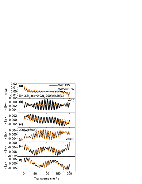
Figure 1: a), b), c) are the spin polarization(x=10) for 200$\times$20, while d), e), f)(x=300) for 200$\times$600, with the unit $\hbar/2$. The continuous line included the evanescent waves(EW). The dotted line included only the extending states.

where $A$ and $B$ are two $4\times 4$ sub-matrix, $A^{\ast}(B^{\ast})$ is the complex conjugate matrix of $A$ $(B)$.

$$A=\left(\begin{array}[]{cccc}a&b&e&f\\ 1&0&0&0\\ -e&-f&a&b\\ 0&0&1&0\end{array}\right),B=\left(\begin{array}[]{cccc}g&0&h&0\\ 0&0&0&0\\ -h^{\ast}&0&g^{\ast}&0\\ 0&0&0&0\end{array}\right)$$ (13)

where $\left\{a,b,e,f,g,h\right\}$ are the functions of the hopping constant $t_{0}$, SOC strength ($t_{so}$ in Rashba region, $0$ in lead region) and eigen energy $E$. The expressions of $\left\{a,b,e,f,g,h\right\}$ are $a=-c\left(E-w_{x,y}\right)/t_{0},b=c\left(t_{so}^{2}/t_{0}^{2}-1\right)$, $e=-ct_{so}\left(E-w_{x,y}\right)/t_{0}^{2},$ $f=-2ct_{so}$ $/t_{0}$, $g=c\left(it_{so}^{2}/t_{0}^{2}-1\right)$, $h=-c\left(1-i\right)t_{so}/t_{0},$and $c=\left(1+t_{so}^{2}/t_{0}^{2}\right)^{-1}$, where $t_{0}=\hbar^{2}/2m^{\ast}a^{2}$, $t_{so}=\alpha/2a$. $w_{x,y}$ is the on-site energy, here we have chosen it to be zero.

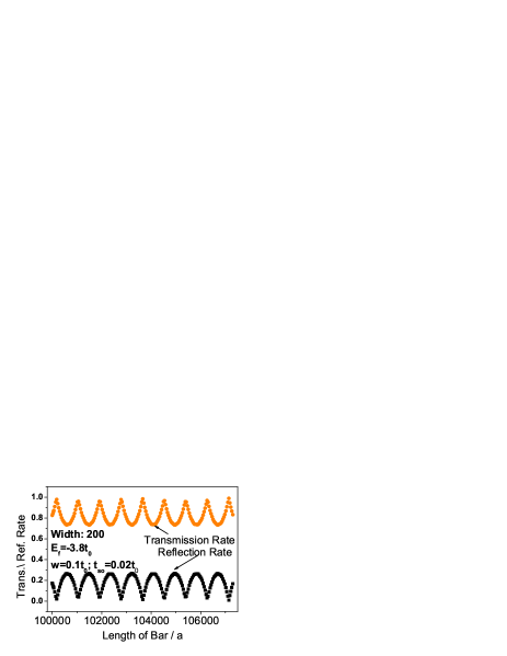
Figure 2: The upper orange line stands for transmission rate, while the lower black line is the reflection rate.

We take the $E$ to be Fermi energy $E_{F},$ and fix the other parameters in TM, then consider an electron wave injecting from one of the channels in left lead and calculate the reflection and transmission coefficients $\{r_{i},t_{i}\}$. Finally the wave functions at every site of the strip can be obtained. We compare the result of our new improved method with that of the OTMM for $2L\leq 15$ for $N=200$ system within which the calculation of OTMM is accurate and has no numerical instability. We obtain the exact same results for the transmission and reflection coefficients. However, our new method can accurately calculate the case of $2L$ as large as we want. Main cost of computer time is from the diagonalization of $800\times 800$ TM. It is clearly shown that our new method does not require more computer time when the length of middle bar increases. Figure  1 and  2 give the exact solution of the spin polarization in middle bar and resonant transmission of current as a function of bar length up to $10^{5}$ lattices, which is a size that can not be calculated by other methods. Where we have taken the average for non-polarized injection. The contribution from evanescent waves to spin polarization of Rashba SOC system based on continuous version has been studied by Li and YangLiYang . From our results of figure 1, the exact calculation shows that the contribution from evanescent wave is significant for a short bar, but it is small when the length of bar becomes long.

Comparison between our new method and previous methods (SMM and ETMT). SMM has been mostly applied for studying the wave transport and has no problem of numerical instabiltyPendry[94] . In SMM, in order to avoid the numerical instability, one has to divide the middle bar into many small sections. Then one should find the SM for each section via TMM. In the sample with $N=100,$ the longest length of such pieces should be less than $400$ lattices such that no numerical instability happens. Here we use the 300 to ensure the precision of calculation. Then a recursion approach is applied to combine every sub SM to reach the final total SMSMM . Fig. 3 shows that the CPU cost of SMM linearly increases with growing length of scattering region, but our new TMM is independent of the length of middle bar as showed in same figure. The numerical solutions obtained by SMM and our new TMM are exactly the same. In addition, when one studies the transmission of a polarized incident wave going through the middle bar, considering only a single channel injection of electron wave is not sufficient for SMM. All channels injection from left and right must be calculated individually to obtain the SM. Thus, the computing time to obtain the SM of first block near interface is almost 4N times of NITMM. Further more, computing time grows linearly for adding every block by recursive algorithm in SMM. In ETMTWan[1998] , they studied the magnetoconductance of a quantum wire with several antidots. The numerical technique used there could avoid numerical instability happened in original transfer-matrix method, and was applied to a variety of 3D systems involving complicated atomic and many-body potentials. However, due to its iterative calculations, the computing time of ETMT also increases linearly with the increase in the length of quantum wire even for the homogeneous region. Our method shows the superiority in treating long homogeneous transfer region for that it does not cost extra computing time as the length of homogeneous scattering region becomes large. The computing time is in the zeroth order of homogenous region length L, $O(L^{0}).$ For the model we calculated here, our method is much faster than SMM for long length system, and we believe that it is also faster than ETMT.

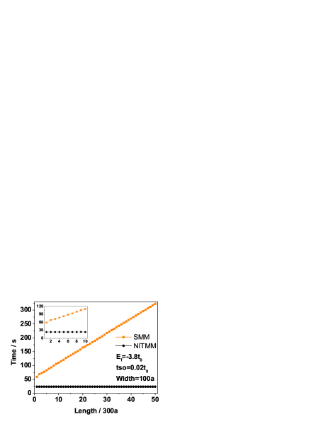
Figure 3: The time cost of SMM(orange upper) increases as the first order of lengths of scattering region, where as that of NITMM(black below) is the zeroth. The maximum length of a single block within which the SMM is applicable is less than 400a, for that there is a matrix inversion operation in the SMM formulae  SMM . Here we choose the maximum length as 300a to ensure the precision of calculation.

Our method can also be applied to the studies on the transport under uniform magnetic field. Extensions of our NITMM to other problems will be our future work.

- (1) Schultz T. D., Mattis D. C. Lieb E. H. Rev. Mod. Phys. 36, 856(1964).
- (2) Morgenstern I. Binder K. Phys.Rev.Lett. 43, 1615(1979).
- (3) Morgenstern I. Binder K. Phys.Rev.B. 22, 288(1980).
- (4) Cheung H.-F. McMillan W. L. J.Phys.C: Solid State Phys. 16, 7027(1983).
- (5) Suzuki M. Phys.Rev.B. 31, 2957(1985).
- (6) Sautet P. Joachim C. Phys.Rev.B 38, 12238(1988).
- (7) Wan C.C., T. D. Jesus and Guo H.Phys.Rev.B 57, 11907(1998).
- (8) Tao R. J.Phys.A: Math.&Gen. 27, 5069(1994).
- (9) Huang X. Gong C. Phys.Rev.B 58, 739(1998).
- (10) Chilwell J. Hodgkinson I. J.Opt.Soc.Am.A 1, 742(1984).
- (11) Wang L. Rokhlin S. I. Ultrasonics 39, 413(2001).
- (12) Li Z.-Y. Lin L.-L. Phys. Rev.E 67, 046607(2003).
- (13) Pendry J. B. Journal of Mordern Optics 41, 209(1994).
- (14) Pendry J. B. MacKinnon A. Phys. Rev. Lett. 69, 2772(1992).
- (15) Bell P. M., Pendry J. B., Moreno L. M. Ward A.J. Comp. Phys. Comm. 85, 306(1995).
- (16) Thouless D. J. Kirkpatrick S. J.Phys.C 14, 235(1981).
- (17) Wu H. Sprung D. W. L. Appl.Phys.A 58, 581(1994).
- (18) Yao J. Yang Z. Phys. Rev. B 73, 033314(2006).
- (19) Li Z. Yang Z. Phys. Rev. B 76, 033307(2007).
- (20) Rashba E. I. Sov. Phys. Solid State 2, 1109(1960).
- (21) The detail formulae of recursive SMM can be found on page 223, formulae (56), Ref.13