Distribution functions of linear combinations of lattice polynomials from the uniform distribution

Abstract

We give the distribution functions, the expected values, and the moments of linear combinations of lattice polynomials from the uniform distribution. Linear combinations of lattice polynomials, which include weighted sums, linear combinations of order statistics, and lattice polynomials, are actually those continuous functions that reduce to linear functions on each simplex of the standard triangulation of the unit cube. They are mainly used in aggregation theory, combinatorial optimization, and game theory, where they are known as discrete Choquet integrals and Lovász extensions.

1 Introduction

Let $h:[0,1]^{n}\to\mathbb{R}$ be an aggregation function and let $\mathbf{X}$ be a random vector uniformly distributed on $[0,1]^{n}$. An interesting but generally difficult problem is to provide explicit expressions for the distribution function and the moments of the aggregated random variable $Y=h(\mathbf{X})$.

This problem has been completely solved for certain aggregation functions (see for instance [21, §7.2]), especially piecewise linear functions such as weighted sums [5] (see also [19]), linear combinations of order statistics [2, 20, 25] (see also [7, §6.5] for an overview), and lattice polynomials [18], which are max-min combinations of the variables.

In this note we solve the case of linear combinations of lattice polynomials, which include the three above-mentioned cases. Actually, linear combinations of lattice polynomials are exactly those continuous functions that reduce to linear functions on each simplex of the standard triangulation of $[0,1]^{n}$. In particular, these functions are completely determined by their values at the $2^{n}$ vertices of $[0,1]^{n}$.

The concept of linear combination of lattice polynomials is known in combinatorial optimization and game theory as the Lovász extension [3, 13, 15, 23] of a pseudo-Boolean function (recall that a pseudo-Boolean function is a real-valued function of 0-1 variables). When it is nondecreasing in each variable, it is known in the area of nonlinear aggregation and integration as the discrete Choquet integral [10, 14, 16], which is an extension of the discrete Lebesgue integral (weighted mean) to non-additive measures. The equivalence between the Lovász extension and the Choquet integral is discussed in [16].

This note is set out as follows. In Section 2 we elaborate on the definition of linear combinations of lattice polynomials and we show how to concisely represent them. In Section 3 we provide formulas for the distribution function and the moments of any linear combination of lattice polynomials from the uniform distribution. Finally, in Section 4 we provide an application of our results to aggregation theory.

Throughout we will use the notation $[n]:=\{1,\ldots,n\}$. Also, for any subset $A\subseteq[n]$, $\mathbf{1}_{A}$ will denote the characteristic vector of $A$ in $\{0,1\}^{n}$. Finally, for any function $h:[0,1]^{n}\to\mathbb{R}$, we define the set function $v_{h}:2^{[n]}\to\mathbb{R}$ as $v_{h}(A):=h(\mathbf{1}_{A})$ for all $A\subseteq[n]$.

2 Linear combinations of lattice polynomials

In the present section we recall the definition of lattice polynomials and we show how an arbitrary combination of lattice polynomials can be represented.

Basically an $n$-place lattice polynomial $p:[0,1]^{n}\to[0,1]$ is a function defined from any well-formed expression involving $n$ real variables $x_{1},\ldots,x_{n}$ linked by the lattice operations $\wedge=\min$ and $\vee=\max$ in an arbitrary combination of parentheses (see e.g. Birkhoff [6, §II.2]). For instance,

$$p(x_{1},x_{2},x_{3})=(x_{1}\wedge x_{2})\vee x_{3}$$

is a 3-place lattice polynomial.

Consider the standard triangulation of $[0,1]^{n}$ into the canonical simplices

$$S_{\sigma}:=\{x\in[0,1]^{n}\mid x_{\sigma(1)}\geqslant\cdots\geqslant x_{\sigma(n)}\}\qquad(\sigma\in\mathfrak{S}_{n}),$$ (1)

where $\mathfrak{S}_{n}$ is the set of all permutations on $[n]$. Clearly, any linear combination of $n$-place lattice polynomials

$$h(\mathbf{x})=\sum_{i=1}^{m}c_{i}\,p_{i}(\mathbf{x})$$

is a continuous function whose restriction to any canonical simplex is a linear function. According to Singer [23, §2], $h$ is then the Lovász extension of the pseudo-Boolean function $h|_{\{0,1\}^{n}}$, that is, the continuous function defined on each canonical simplex $S_{\sigma}$ as the unique linear function that coincides with $h|_{\{0,1\}^{n}}$ at the $n+1$ vertices

$$\varepsilon_{i}^{\sigma}:=\mathbf{1}_{\{\sigma(1),\ldots,\sigma(i)\}}\qquad(i=0,\ldots,n)$$

of $S_{\sigma}$. It can be written as [23, §2]

$$h(\mathbf{x})=\sum_{i=1}^{n}\big{(}h_{i}^{\sigma}-h_{i-1}^{\sigma}\big{)}\,x_{\sigma(i)}\qquad(\mathbf{x}\in S_{\sigma}),$$ (2)

where $h_{i}^{\sigma}:=h\big{(}\varepsilon_{i}^{\sigma}\big{)}=v_{h}\big{(}\{\sigma(1),\ldots,\sigma(i)\}\big{)}$ for all $i=0,\ldots,n$. In particular, $h_{0}^{\sigma}=0$.

Conversely any continuous function $h:[0,1]^{n}\to\mathbb{R}$ that reduces to a linear function on each canonical simplex is a linear combination of lattice polynomials:

$$h(\mathbf{x})=\sum_{A\subseteq[n]}m_{h}(A)\,\bigwedge_{i\in A}x_{i}\qquad(\mathbf{x}\in[0,1]^{n}),$$ (3)

where $m_{h}:2^{[n]}\to\mathbb{R}$ is the Möbius transform of $v_{h}$, defined as

$$m_{h}(A):=\sum_{B\subseteq A}(-1)^{|A|-|B|}v_{h}(B).$$

Indeed, expression (3) reduces to a linear function on each canonical simplex and agrees with $h(\mathbf{1}_{B})$ at $\mathbf{1}_{B}$ for each $B\subseteq[n]$.

Eq. (2) thus provides a concise expression for linear combinations of lattice polynomials. We will use it in the next section to calculate their distribution functions and their moments.

Remark 1

As we have already mentioned, the class of linear combinations of lattice polynomials covers three interesting particular cases, namely: lattice polynomials, linear combinations of order statistics, and weighted sums. These are characterized as follows. Let $h:[0,1]^{n}\to\mathbb{R}$ be a linear combination of lattice polynomials.

1. The function $h$ reduces to a lattice polynomial if and only if the set function $v_{h}$ is monotone, $\{0,1\}$-valued, and such that $v_{h}([n])=1$.

2. As the order statistics are exactly the symmetric lattice polynomials (see [17]), the function $h$ reduces to a linear combination of order statistics if and only if the set function $v_{h}$ is cardinality-based, that is, such that $v_{h}(A)=v_{h}(A^{\prime})$ whenever $|A|=|A^{\prime}|$.

3. The function $h$ reduces to a weighted sum if and only if the set function $v_{h}$ is additive, that is, $v_{h}(A)=\sum_{i\in A}v_{h}(\{i\})$.

3 Distribution functions and moments

Before yielding the main results, let us recall some basic material related to divided differences. See for instance [8, 11, 22] for further details.

Consider the plus (resp. minus) truncated power function $x^{n}_{+}$ (resp. $x^{n}_{-}$), defined to be $x^{n}$ if $x>0$ (resp. $x<0$) and zero otherwise. Let $\mathcal{A}^{(n)}$ be the set of $n-1$ times differentiable one-place functions $g$ such that $g^{(n-1)}$ is absolutely continuous. The $n$th divided difference of a function $g\in\mathcal{A}^{(n)}$ is the symmetric function of $n+1$ arguments defined inductively by $\Delta[g:a_{0}]:=g(a_{0})$ and

$$\Delta[g:a_{0},\ldots,a_{n}]:=\begin{cases}\displaystyle{\frac{\Delta[g:a_{1},\ldots,a_{n}]-\Delta[g:a_{0},\ldots,a_{n-1}]}{a_{n}-a_{0}}},&\mbox{if $a_{0}\neq a_{n}$},\\ \displaystyle{\frac{\partial}{\partial a_{0}}\,\Delta[g:a_{0},\ldots,a_{n-1}]},&\mbox{if $a_{0}=a_{n}$.}\end{cases}$$

The Peano representation of the divided differences, which can be obtained by a Taylor expansion of $g$, is given by

$$\Delta[g:a_{0},\ldots,a_{n}]=\frac{1}{n!}\,\int_{\mathbb{R}}g^{(n)}(t)\,M(t\mid a_{0},\ldots,a_{n})\,\mathrm{d}t,$$ (4)

where $M(t\mid a_{0},\ldots,a_{n})$ is the B-spline of order $n$, with knots $\{a_{0},\ldots,a_{n}\}$, defined as

$$M(t\mid a_{0},\ldots,a_{n}):=n\,\Delta[(\boldsymbol{\cdot}-t)^{n-1}_{+}:a_{0},\ldots,a_{n}].$$ (5)

We also recall the Hermite-Genocchi formula: For any function $g\in\mathcal{A}^{(n)}$, we have

$$\Delta[g:a_{0},\ldots,a_{n}]=\int_{S_{id}}g^{(n)}\Big{[}a_{0}+\sum_{i=1}^{n}(a_{i}-a_{i-1})x_{i}\Big{]}\,\mathrm{d}\mathbf{x},$$ (6)

where $S_{id}$ is the simplex defined in (1) when $\sigma$ is the identity permutation.

For distinct arguments $a_{0},\ldots,a_{n}$, we also have the following formula, which can be verified by induction,

$$\Delta[g:a_{0},\ldots,a_{n}]=\sum_{i=0}^{n}\frac{g(a_{i})}{\prod_{j\neq i}(a_{i}-a_{j})}.$$ (7)

Now, consider a random vector $\mathbf{X}$ uniformly distributed on $[0,1]^{n}$ and set $Y_{h}:=h(\mathbf{X})$, where the function $h:[0,1]^{n}\to\mathbb{R}$ is a linear combination of lattice polynomials as given in formula (2). We then have the following result.

Theorem 2

For any function $g\in\mathcal{A}^{(n)}$, we have

$$\mathbf{E}[g^{(n)}(Y_{h})]=\sum_{\sigma\in\mathfrak{S}_{n}}\Delta[g:h_{0}^{\sigma},\ldots,h_{n}^{\sigma}].$$ (8)

Proof. Using (2), we simply have

$$\mathbf{E}[g^{(n)}(Y_{h})] = \int_{[0,1]^{n}}g^{(n)}[h(\mathbf{x})]\,{\rm d}\mathbf{x}$$

$$= \sum_{\sigma\in\mathfrak{S}_{n}}\int_{S_{\sigma}}g^{(n)}\Big{[}\sum_{i=1}^{n}\big{(}h_{i}^{\sigma}-h_{i-1}^{\sigma}\big{)}x_{\sigma(i)}\Big{]}\,{\rm d}\mathbf{x}.$$

Finally, after an elementary change of variables, we conclude by the Hermite-Genocchi formula (6).∎

Theorem 2 provides the expectation $\mathbf{E}[g^{(n)}(Y_{h})]$ in terms of the divided differences of $g$ with arguments $h_{0}^{\sigma},\ldots,h_{n}^{\sigma}$ $(\sigma\in\mathfrak{S}_{n})$. An explicit formula can be obtained by (7) whenever the arguments are distinct for every $\sigma\in\mathfrak{S}_{n}$.

Clearly, the special cases

$$g(x)=\frac{r!}{(n+r)!}\,x^{n+r},~{}\frac{r!}{(n+r)!}\,[x-\mathbf{E}(Y_{h})]^{n+r},~{}\mbox{and}~{}\frac{e^{tx}}{t^{n}}$$ (9)

give, respectively, the raw moments, the central moments, and the moment-generating function of $Y_{h}$. As far as the raw moments are concerned, we have the following result.

Proposition 3

For any integer $r\geqslant 1$, setting $A_{0}:=[n]$, we have,

$$\mathbf{E}[Y_{h}^{r}]=\frac{1}{{n+r\choose r}}\sum_{{A_{1}\subseteq[n]\atop A_{2}\subseteq A_{1}}\atop{\cdots\atop A_{r}\subseteq A_{r-1}}}\,\prod_{i=1}^{r}\frac{1}{{|A_{i-1}|\choose|A_{i}|}}\,v_{h}(A_{i}).$$

Proof. Let $r\geqslant 1$. It can be shown [4] that

$$\Delta[(\boldsymbol{\cdot})^{n+r}:a_{0},\ldots,a_{n}]=\sum_{\textstyle{r_{0},\ldots,r_{n}\geqslant 0\atop r_{0}+\cdots+r_{n}=r}}a_{0}^{r_{0}}\cdots a_{n}^{r_{n}}=\sum_{0\leqslant i_{1}\leqslant\cdots\leqslant i_{r}\leqslant n}a_{i_{1}}\cdots a_{i_{r}}.$$

Hence, from (8) and (9) it follows that

$$\mathbf{E}[Y_{h}^{r}] = \frac{r!}{(n+r)!}\,\sum_{0\leqslant i_{1}\leqslant\cdots\leqslant i_{r}\leqslant n}\,\sum_{\sigma\in\mathfrak{S}_{n}}h_{i_{1}}^{\sigma}\cdots h_{i_{r}}^{\sigma}$$

$$= \frac{r!}{(n+r)!}\,\sum_{0\leqslant i_{1}\leqslant\cdots\leqslant i_{r}\leqslant n}\,\sum_{m\in\mathcal{M}_{n}}v_{h}(m_{i_{1}})\cdots v_{h}(m_{i_{r}}),$$

where $\mathcal{M}_{n}$ is the set of the $n!$ maximal chains of the lattice $(2^{[n]},\subseteq)$, and where, for any $m\in\mathcal{M}_{n}$, $m_{i}$ is the unique element of $m$ of cardinality $i$.

For any $B_{1}\subseteq\dots\subseteq B_{r}\subseteq[n]$, let $\mathcal{M}_{n}^{B_{1},\dots,B_{r}}$ denote the subset of maximal chains of $(2^{[n]},\subseteq)$ containing $B_{1},\dots,B_{r}$. It is then easy to see that, for any fixed $0\leqslant i_{1}\leqslant\cdots\leqslant i_{r}\leqslant n$, the following identity holds:

$$\bigcup_{\textstyle{B_{1}\subseteq\dots\subseteq B_{r}\subseteq[n]\atop|B_{1}|=i_{1},\dots,|B_{r}|=i_{r}}}\mathcal{M}_{n}^{B_{1},\dots,B_{r}}=\mathcal{M}_{n}$$

and the union is disjoint. Therefore, we have

$$\mathbf{E}[Y_{h}^{r}] = \frac{r!}{(n+r)!}\,\sum_{0\leqslant i_{1}\leqslant\cdots\leqslant i_{r}\leqslant n}\,\sum_{\textstyle{B_{1}\subseteq\dots\subseteq B_{r}\subseteq[n]\atop|B_{1}|=i_{1},\dots,|B_{r}|=i_{r}}}\,\sum_{m\in\mathcal{M}_{n}^{B_{1},\dots,B_{r}}}v_{h}(B_{1})\cdots v_{h}(B_{r})$$

$$= \frac{r!}{(n+r)!}\,\sum_{B_{1}\subseteq\dots\subseteq B_{r}\subseteq[n]}|\mathcal{M}_{n}^{B_{1},\dots,B_{r}}|\,\prod_{i=1}^{r}v_{h}(B_{i}),$$

where

$$|\mathcal{M}_{n}^{B_{1},\dots,B_{r}}|=|B_{1}|!\,(|B_{2}|-|B_{1}|)!\,(|B_{3}|-|B_{2}|)!\,\cdots(n-|B_{r}|)!.$$

Finally, we get the result by setting $A_{i}:=B_{r+1-i}$ for all $i=1,\ldots,r$.∎

Proposition 3 provides an explicit expression for the $r$th raw moment of $Y_{h}$ as a sum of $(r+1)^{n}$ terms. For instance, the first two moments are

$$\mathbf{E}[Y_{h}] = \frac{1}{n+1}\,\sum_{A\subseteq[n]}\frac{1}{{n\choose|A|}}\,v_{h}(A),$$

$$\mathbf{E}[Y_{h}^{2}] = \frac{2}{(n+1)(n+2)}\,\sum_{A_{1}\subseteq[n]}\frac{1}{{n\choose|A_{1}|}}\,v_{h}(A_{1})\sum_{A_{2}\subseteq A_{1}}\frac{1}{{|A_{1}|\choose|A_{2}|}}\,v_{h}(A_{2}).$$

We now yield a formula for the distribution function $F_{h}(y):=\Pr[Y_{h}\leqslant y]$ of $Y_{h}$.

Theorem 4

There holds

$$F_{h}(y)=1-\frac{1}{n!}\,\sum_{\sigma\in\mathfrak{S}_{n}}\Delta[(\boldsymbol{\cdot}-y)^{n}_{+}:h_{0}^{\sigma},\ldots,h_{n}^{\sigma}].$$ (10)

Proof. We have

$$F_{h}(y)=1-\Pr[h(\mathbf{X})>y]=1-\mathbf{E}\big{[}(Y_{h}-y)^{0}_{+}\big{]}.$$

Then, using (8) with

$$g(x)=\frac{1}{n!}\,(x-y)^{n}_{+}$$

leads to the result.∎

It follows from (10) that the distribution function of $Y_{h}$ is absolutely continuous and hence its probability density function is simply given by

$$f_{h}(y)=\frac{1}{(n-1)!}\,\sum_{\sigma\in\mathfrak{S}_{n}}\Delta[(\boldsymbol{\cdot}-y)^{n-1}_{+}:h_{0}^{\sigma},\ldots,h_{n}^{\sigma}]$$ (11)

or, using the B-spline notation (5),

$$f_{h}(y)=\frac{1}{n!}\,\sum_{\sigma\in\mathfrak{S}_{n}}M(y\mid h_{0}^{\sigma},\ldots,h_{n}^{\sigma}).$$

Remark 5

1. It is easy to see that (10) can be rewritten by means of the minus truncated power function as

   $$F_{h}(y)=\frac{1}{n!}\,\sum_{\sigma\in\mathfrak{S}_{n}}\Delta[(\boldsymbol{\cdot}-y)^{n}_{-}:h_{0}^{\sigma},\ldots,h_{n}^{\sigma}].$$

2. When the arguments $h_{0}^{\sigma},\ldots,h_{n}^{\sigma}$ are distinct for every $\sigma\in\mathfrak{S}_{n}$, then combining (7) with (10) immediately yields the following explicit expression

   $$F_{h}(y)=1-\frac{1}{n!}\,\sum_{\sigma\in\mathfrak{S}_{n}}\sum_{i=0}^{n}\frac{(h_{i}^{\sigma}-y)^{n}_{+}}{\prod_{j\neq i}(h_{i}^{\sigma}-h_{j}^{\sigma})},$$

   or, using the minus truncated power function,

   $$F_{h}(y)=\frac{1}{n!}\,\sum_{\sigma\in\mathfrak{S}_{n}}\sum_{i=0}^{n}\frac{(h_{i}^{\sigma}-y)^{n}_{-}}{\prod_{j\neq i}(h_{i}^{\sigma}-h_{j}^{\sigma})}.$$

3. The knowledge of $f_{h}(y)$ immediately gives an alternative proof of (8). Indeed, using Peano’s representation (4), we simply have

   $$\mathbf{E}[g^{(n)}(Y_{h})] = \int_{\mathbb{R}}g^{(n)}(y)\,f_{h}(y)\,\mathrm{d}y$$

   $$= \frac{1}{n!}\sum_{\sigma\in\mathfrak{S}_{n}}\int_{\mathbb{R}}g^{(n)}(y)\,M(y\mid h_{0}^{\sigma},\ldots,h_{n}^{\sigma})\,\mathrm{d}y$$

   $$= \sum_{\sigma\in\mathfrak{S}_{n}}\Delta[g:h_{0}^{\sigma},\ldots,h_{n}^{\sigma}].$$

4. The case of linear combinations of order statistics is of particular interest. In this case, each $h_{i}^{\sigma}$ is independent of $\sigma$ (see Remark 1), so that we can write $h_{i}:=h_{i}^{\sigma}$. The main formulas then reduce to (see for instance [1] and [2])

   $$\mathbf{E}[g^{(n)}(Y_{h})] = n!\,\Delta[g:h_{0},\ldots,h_{n}],$$

   $$F_{h}(y) = \Delta[(\boldsymbol{\cdot}-y)^{n}_{-}:h_{0},\ldots,h_{n}],$$

   $$f_{h}(y) = M(y\mid h_{0},\ldots,h_{n}).$$

   We also note that the Hermite-Genocchi formula (6) provides nice geometric interpretations of $F_{h}(y)$ and $f_{h}(y)$ in terms of volumes of slices and sections of canonical simplices (see also [4] and [12]).

Both functions $F_{h}(y)$ and $f_{h}(y)$ require the computation of divided differences of truncated power functions. On this issue, we recall a recurrence equation, due to de Boor [9] and rediscovered independently by Varsi [24] (see also [4]), which allows to compute $\Delta[(\boldsymbol{\cdot}-y)^{n-1}_{+}:a_{0},\ldots,a_{n}]$ in $O(n^{2})$ time.

Rename as $b_{1},\dots,b_{r}$ the elements $a_{i}$ such that $a_{i}<y$ and as $c_{1},\dots,c_{s}$ the elements $a_{i}$ such that $a_{i}\geqslant y$ so that $r+s=n+1$. Then, the unique solution of the recurrence equation

$$\alpha_{k,l}=\frac{(c_{l}-y)\alpha_{k-1,l}+(y-b_{k})\alpha_{k,l-1}}{c_{l}-b_{k}}\qquad(k\leqslant r,\,l\leqslant s),$$ (12)

with initial values $\alpha_{1,1}=(c_{1}-b_{1})^{-1}$ and $\alpha_{0,l}=\alpha_{k,0}=0$ for all $l,k\geqslant 2$, is given by

$$\alpha_{k,l}:=\Delta[(\boldsymbol{\cdot}-y)_{+}^{k+l-2}:b_{1},\dots,b_{k},c_{1},\dots,c_{l}]\qquad(k+l\geqslant 2).$$

In order to compute $\Delta[(\boldsymbol{\cdot}-y)^{n-1}_{+}:a_{0},\ldots,a_{n}]=\alpha_{r,s}$, it suffices therefore to compute the sequence $\alpha_{k,l}$ for $k+l\geqslant 2$, $k\leqslant r$, $l\leqslant s$, by means of two nested loops, one on $k$, the other on $l$.

We can compute $\Delta[(\boldsymbol{\cdot}-y)^{n}_{-}:a_{0},\ldots,a_{n}]$ similarly. Indeed, the same recurrence equation applied to the initial values $\alpha_{0,l}=0$ for all $l\geqslant 1$ and $\alpha_{k,0}=1$ for all $k\geqslant 1$, produces the solution

$$\alpha_{k,l}:=\Delta[(\boldsymbol{\cdot}-y)_{-}^{k+l-1}:b_{1},\dots,b_{k},c_{1},\dots,c_{l}]\qquad(k+l\geqslant 1).$$

See for instance [4] and [24] for further details.

4 Application to aggregation theory

As we have already mentioned, the concept of linear combination of lattice polynomials, when it is nondecreasing in each variable, is known in aggregation theory as the discrete Choquet integral, which is extensively used in non-additive expected utility theory, cooperative game theory, complexity analysis, measure theory, etc. (see [14] for an overview.) For instance, when a discrete Choquet integral is used as an aggregation tool in a given decision making problem, it is then very informative for the decision maker to know its distribution. In that context, the most natural a priori density on $[0,1]^{n}$ is the uniform one, which makes the results derived here of particular interest.

Example 6

Let $h:[0,1]^{3}\to\mathbb{R}$ be a discrete Choquet integral defined by $v_{h}(\{1\})=0.1$, $v_{h}(\{2\})=0.6$, $v_{h}(\{3\})=v_{h}(\{1,2\})=v_{h}(\{1,3\})=v_{h}(\{2,3\})=0.9$, and $v_{h}(\{1,2,3\})=1$. According to (3), it can be written as

$$h(\mathbf{x}) = 0.1\,x_{1}+0.6\,x_{2}+0.9\,x_{3}$$

$$\hbox{}+0.2(x_{1}\wedge x_{2})-0.1(x_{1}\wedge x_{3})-0.6(x_{2}\wedge x_{3})$$

$$\hbox{}-0.1(x_{1}\wedge x_{2}\wedge x_{3}).$$

Its density, which can be computed through (11) and the recurrence equation (12), is represented in Figure 1 by the solid line. The dotted line represents the density estimated by the kernel method from 10 000 randomly generated realizations. The typical value and standard deviation can also be calculated through the raw moments: we have

$$\mathbf{E}[Y_{h}]\approx 0.608\quad\mbox{and}\quad\sqrt{\mathbf{E}[Y_{h}^{2}]-\mathbf{E}[Y_{h}]^{2}}\approx 0.204.$$

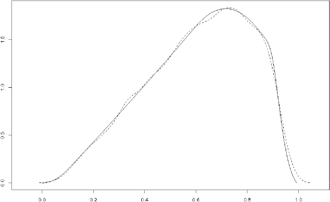
Figure 1: Density of a discrete Choquet integral (solid line).

References

• [1] J. A. Adell and C. Sangüesa. Error bounds in divided difference expansions. A probabilistic perspective. J. Math. Anal. Appl., 318(1):352–364, 2006.
• [2] G. G. Agarwal, R. J. Dalpatadu, and A. K. Singh. Linear functions of uniform order statistics and B-splines. Commun. Stat., Theory Methods, 31(2):181–192, 2002.
• [3] E. Algaba, J. Bilbao, J. Fernández, and A. Jiménez. The Lovász extension of market games. Theory Decis., 56(1-2):229–238, 2004.
• [4] M. M. Ali. Content of the frustum of a simplex. Pac. J. Math., 48:313–322, 1973.
• [5] D. Barrow and P. Smith. Spline notation applied to a volume problem. Am. Math. Mon., 86:50–51, 1979.
• [6] G. Birkhoff. Lattice theory. Third edition. American Mathematical Society Colloquium Publications, Vol. XXV. American Mathematical Society, Providence, R.I., 1967.
• [7] H. David and H. Nagaraja. Order statistics. 3rd ed. Wiley Series in Probability and Statistics. Chichester: John Wiley & Sons., 2003.
• [8] P. J. Davis. Interpolation and approximation. 2nd ed. Dover Books on Advanced Mathematics. New York: Dover Publications, 1975.
• [9] C. de Boor. On calculating with B-splines. J. Approximation Theory, 6:50–62, 1972.
• [10] D. Denneberg. Non-additive measure and integral. Theory and Decision Library. Series B: Mathematical and Statistical Methods. 27. Dordrecht: Kluwer Academic Publishers, 1994.
• [11] R. A. DeVore and G. G. Lorentz. Constructive approximation. Berlin: Springer-Verlag, 1993.
• [12] L. Gerber. The volume cut off a simplex by a half-space. Pac. J. Math., 94:311–314, 1981.
• [13] M. Grabisch, J.-L. Marichal, and M. Roubens. Equivalent representations of set functions. Math. Oper. Res., 25(2):157–178, 2000.
• [14] M. Grabisch, T. Murofushi, and M. Sugeno, editors. Fuzzy measures and integrals, volume 40 of Studies in Fuzziness and Soft Computing. Physica-Verlag, Heidelberg, 2000. Theory and applications.
• [15] L. Lovász. Submodular functions and convexity. In Mathematical programming, 11th int. Symp., Bonn 1982, 235–257. 1983.
• [16] J.-L. Marichal. Aggregation of interacting criteria by means of the discrete Choquet integral. In Aggregation operators: new trends and applications, pages 224–244. Physica, Heidelberg, 2002.
• [17] J.-L. Marichal. On order invariant synthesizing functions. J. Math. Psych., 46(6):661–676, 2002.
• [18] J.-L. Marichal. Cumulative distribution functions and moments of lattice polynomials. Statistics & Probability Letters, 76(12):1273–1279, 2006.
• [19] J.-L. Marichal and M. Mossinghoff. Slices, slabs, and sections of the unit hypercube. Submitted for publication. http://arxiv.org/abs/math/0607715
• [20] T. Matsunawa. The exact and approximate distributions of linear combinations of selected order statistics from a uniform distribution. Ann. Inst. Stat. Math., 37:1–16, 1985.
• [21] J. H. McColl. Multivariate probability. Arnold Texts in Statistics. London: Arnold, 2004.
• [22] M. Powell. Approximation theory and methods. Cambridge University Press, 1981.
• [23] I. Singer. Extensions of functions of 0-1 variables and applications to combinatorial optimization. Numer. Funct. Anal. Optimization, 7:23–62, 1984.
• [24] G. Varsi. The multidimensional content of the frustum of the simplex. Pac. J. Math., 46:303–314, 1973.
• [25] H. Weisberg. The distribution of linear combinations of order statistics from the uniform distribution. Ann. Math. Statist., 42:704–709, 1971.