A fast simulator for polycrystalline processes with application to phase change alloys

Abstract

We present a stochastic simulator for polycrystalline phase-change materials capable of spatio-temporal modelling of complex anneals. This is based on consideration of bulk and surface energies to generate rates of growth and decay of crystallites built up of ‘monomers’ that themselves may be quite complex molecules. We perform a number of simulations of this model using a Gillespie algorithm. The simulations are performed at molecular scale and using an approximation of local free energy changes that depend only on immediate neighbours. The sites are on a lattice chosen to have a lengthscale of the individual monomers, where each site gives information about a two-state local phase $r$ ($r=0$ corresponds to amorphous and $1$ corresponds to crystalline) and a continuous crystal orientation $\phi$ at each site.

As an example we use this to model crystallisation in chalcogenide GST ($GeSbTe$) alloys used for example in phase-change memory devices, where reversible changes between amorphous and crystalline regimes are used to store and process information. We use our model to simulate anneals of GST including ones with non-trivial spatial and temporal variation of temperature; this gives good agreement to experimental incubation times at low temperatures while modelling non-trivial crystal size distributions and melting dynamics at higher temperatures.

I Introduction

This paper considers a model for phase change materials, i.e. alloys that can undergo reversible phase changes in response to anneals. Possible modelling techniques for polycrystalline processes in reversible phase-change alloys such as GST ($GeSbTe$) range from molecular dynamic simulations at one end of the spectrum to empirical models at the other. The former are thermodynamically realistic but highly computer-intensive; the latter are fast, but hard to relate to material properties. Hence models used in practise tend to lie somewhere between the two, for example, Monte Carlo simulations MC_sims , JMAK and master equation based models Ka1 ; KGT ; SW_2004 ; WAB_APL or probabilistic cellular automata pcaref ; YONA ; Hyot&al .

We describe the material as a 2D lattice of discrete ‘sites’ where each site is either crystalline or amorphous and there is an underlying orientation that varies continuously; these sites are on the lengthscale of monomers, though they do not correspond directly to individual monomers. As such our method for generating complex anneals, combines elements of probabilistic cellular automata (PCA) models pcaref ; YONA ; Hyot&al , polycrystalline phase field models KarRap ; CX ; VP_2006 and uses thermodynamics from master equation models Ka1 ; KGT . As we use a Gillespie algorithm for time-stepping we refer to it as a ‘Phase Field Gillespie’ model. In particular we retain a high level of simplicity because of discrete time and lattice space model, while retaining thermodynamic realism and hence keep fitting parameters to a minimum.

Recall that crystallisation can be thought of as a two-stage process; nucleation (where a small crystallite needs to overcome an energy barrier dominated by interfacial energy) and growth (where the crystallite grows according to the availability of neighboring monomers and dominated by bulk energy). We assume each site has a set of locally-determined rate constants for transitions into a new state. These rates depend only on the current state of the site and that of its immediate neighbours. For the rates of growth and dissociation for GST we use thermodynamics from SW_2004 ; WAB_APL .

The Gillespie algorithm GIL_1977 can be used to simulate the evolution under the assumption that the events are independent, instantaneous and never simultaneous. Each step of the algorithm has two parts; firstly it determines a random time to next event and secondly it determines which event occurs. This enables one to perform fast and physically plausible simulations of a number of crystallisation-related phenomena, including incomplete crystallisation, melting and complex spatio-temporal anneals. As there are many possible events, one must efficiently use data-structures to ensure that the simulations run at a high speed and hence perform simulation of complex anneals in 2D on a standard desktop computer.

After the algorithm for the Phase Field Gillespie simulator is described in Section  II, Section III presents the results of some bulk anneals of GST using this simulator, showing that the simulator can model nucleation effects, non-trivial anneals and melting. We include examples where the temperature depends on space and/or time; one can see a variety of effects and a good quantitative agreement with experimental temperature-dependent incubation times for GST. Finally Section IV discusses some possible extensions and limitations of the method.

II A Phase Field Gillespie (PFG) crystallisation simulator

We consider a homogeneous (though not necessarily isotropic) material in 2D. The state of the material is described on a discrete regular lattice of grid points $G$ on the length scale of the individual monomers. Each site is assumed to be either ‘crystalline’ or ‘amorphous’. More precisely, at each grid point, $(i,j)\in G$, the state is described by two quantities:

• $r_{ij}$ – a discrete ‘phase’ variable that is either $0$ (amorphous) or $1$ (crystalline).

• $\phi_{ij}$ – a continuous ‘orientation’ variable that varies over some range $[0,\pi)$ and gives a notional representation for the local orientation of the material.

In particular we can determine that two adjacent crystalline sites are within the same crystal if and only if $r_{ij}=r_{kl}=1$ and $\phi_{ij}=\phi_{kl}$.

The model we describe is a stochastic model that estimates rates of possible local changes to the state of the system (i.e. changes that affect only one site) and uses a Gillespie algorithm GIL_1977 to evolve the system in time. A Gillespie algorithm is optimal in that it will generate timesteps at a rate corresponding to the fastest rate that requires updating, though it is typically more complex to implement than Monte Carlo simulations MC_sims . Although there are adaptations of the algorithm to other contexts Gil_2001 we use the original version of Gillespie.

We consider the following possible instantaneous events at a site $(i,j)\in G$:

• Nucleation – The site $(i,j)$ and an adjacent site, originally both amorphous, become a crystallite at a rate $C^{\rm nu}_{ij}$.

• Growth – The site $(i,j)$, originally amorphous, becomes attached to an adjacent crystal of orientation $\psi$ at a rate $C^{\rm gr}_{ij\psi}$.

• Dissociation – The site $(i,j)$, originally crystalline, detaches or dissociates from the crystal of which it is a part to become amorphous at a rate $C^{\rm di}_{ij}$, and assumes a random orientation.

II.1 The rate coefficients

We approximate the rate coefficients for nucleation, growth and dissociation ($C^{\rm nu}$, $C^{\rm gr}$ and $C^{\rm di}$) at each grid point by considering the change in bulk and surface energies of crystallites adjacent to that site. We define the set of neighbours of $(i,j)\in G$

$$N_{ij}=\{(k,l)\in G:(k,l)\mbox{ is a neighbour of }(i,j)\},\mbox{ and }n_{ij}=|N_{ij}|,$$

the set of amorphous neighbours of $(i,j)$

$$N^{am}_{ij}=\{(k,l)\in N_{ij}:r_{kl}=0\},\mbox{ and }n^{am}_{ij}=|N^{am}_{ij}|,$$

and finally the set of crystalline neighbours of $(i,j)$ with a given orientation $\psi$

$$N^{or}_{ij\psi}=\{(k,l)\in N_{ij}:\phi_{kl}=\psi~{}{\rm and}~{}r_{kl}=1\},\mbox{ and }n^{or}_{ij\psi}=|N^{or}_{ij\psi}|.$$

Note that $n^{am}_{ij},n^{or}_{ij\psi}\in\{0,\cdots,n_{ij}\}$.

The rates are considered in a similar way to the derivation of master equation rates as in SW_2004 and outlined below. We assume that ‘interactions’ between neighbours occur at a temperature-dependent rate

$$R(T)=k_{0}e^{\left(-\frac{E_{a}}{k_{B}T}\right)}$$

where $E_{a}$ is the activation energy and $k_{B}$ is the Boltzmann constant. The prefactor $k_{0}$ is used as a fitting parameter to normalise the results; see SW_2004 .

If adjacent sites have an ‘interaction’ we define

$$\xi(T,A)=\left\{\begin{array}[]{l}\mbox{rate at which a site transforms form amorphous to crystalline,}\\ \mbox{resulting in a change A in surface area of the crystallite}.\end{array}\right\}$$

We assume local thermal equilibrium, meaning that the rate of the reverse transformation at an interaction is $\xi^{-1}(T,A)$. This rate varies with temperature as the bulk and surface energy vary.

We compute the change in surface area of the crystallites on adding site $(i,j)$ to a neighbouring crystal of orientation $\psi$ by a linear approximation

$$A=S_{m}\left[\frac{n_{ij}-2n_{ij\psi}}{n_{ij}}\right]$$

where $S_{m}$ is the surface area of a single site. This means that changing an isolated site in the middle of a crystal of orientation $\psi$ will result in a change $A=-S_{m}$ (as $n_{ij\psi}=n_{ij}$), while creating a new crystal in the middle of a field of amorphous material will result in a change $A=S_{m}$ (as $n_{ij\psi}=0$).

Putting this together (and noting that only by interaction with amorphous neighbours can a site nucleate) we get rate for nucleation that is

$$C^{\rm nu}_{ij}=\left\{\begin{array}[]{ll}k_{0}~{}e^{\left(-\frac{E_{a}}{k_{B}T}\right)}~{}\frac{n^{am}_{ij}}{n_{ij}}\xi(T,S_{m})&\mbox{if}~{}r_{ij}=0\\ 0&\mbox{if}~{}r_{ij}=1.\end{array}\right.$$ (1)

The growth rate for an amorphous site to join a crystalline neighbour with orientation $\psi$ is:

$$C^{\rm gr}_{ij\psi}=\left\{\begin{array}[]{ll}k_{0}~{}e^{\left(-\frac{E_{a}}{k_{B}T}\right)}~{}\xi(T,S_{m}\frac{n_{ij}-2n_{ij\psi}^{or}}{n_{ij}}){}&\mbox{if}~{}r_{ij}=0\\ 0&\mbox{if}~{}r_{ij}=1.\end{array}\right.$$ (2)

Finally, the dissociation rate for a crystalline site to become amorphous is:

$$C^{\rm di}_{ij}=\left\{\begin{array}[]{ll}0&\mbox{if}~{}r_{ij}=0\\ k_{0}~{}e^{\left(-\frac{E_{a}}{k_{B}T}\right)}~{}{\xi(T,S_{m}\frac{n_{ij}-2n_{ij\psi}^{or}}{n_{ij}})^{-1}{}}&\mbox{if}~{}r_{ij}=1.\end{array}\right.$$ (3)

II.2 The PFG Algorithm

We now detail the operation of the PFG algorithm using the rates above. Initially, the whole domain is assumed to be an ‘as deposited’ amorphous state with a random distribution of $\phi_{ij}$ values and $r_{ij}=0$, though one can restart the algorithm from any given state.

For a square lattice we use eight neighbors, $n_{ij}=8$, weighted according to their distance from the site. The new state of the site is then given by $r^{\prime}_{ij}$ and $\phi^{\prime}_{ij}$, using the stochastic simulation algorithm of Gillespie GIL_1977 as follows. This simulates up to a time $T_{\max}$.

1. Start at time $T=0$ with given $r_{ij}$ and $\phi_{ij}$.

2. Generate rate coefficients for all grid points $C_{ij}^{\rm nu}$ $C_{ij\psi}^{\rm gr}$ $C_{ij}^{\rm di}$ for nucleation, growth and dissociation respectively. We refer to these using a single index $\nu=(i,j,{\rm a})$ where ${\rm a}\in\{{\rm nu,(\rm gr,\psi),\rm di}\}$.

3. Compute the sum

   $$a_{0}=\sum C^{\rm nu}_{ij}+\sum_{ij}\left[\sum_{\psi\in\Psi_{ij}}C^{\rm gr}_{ij\psi}\right]+\sum C^{\rm di}_{ij}$$

   where $\Psi_{ij}=\{\phi_{kl}~{}:~{}(k,l)\in N_{ij}\}$ is the set of orientations of neighbours to $(i,j)$.

4. Generate two independent random numbers $\eta_{1},\eta_{2}$ uniformly distributed on $(0,1)$ and compute

   $$d\tau=\frac{1}{a_{0}}\log_{e}\left(\frac{1}{\eta_{1}}\right).$$ (4)

   Increment time to $T=T+d\tau$. If $T\geq T_{\max}$ then stop.

5. Identify the event $\nu=(i,j,{\rm a})$ corresponding to $(i,j)$, ${\rm a}\in{\rm(nu,gr,di)}$ and $(k,l)$ with $\phi_{kl}=\psi$ such that

   $$\sum_{\nu=1}^{\mu-1}{a_{\nu}}<\eta_{2}a_{0}\leq\sum_{\nu=1}^{\mu}{a_{\nu}}$$ (5)

6. Update the value of $\phi_{ij}$ and $r_{ij}$. More precisely, perform the following updates according to corresponding reactions (nucleation, growth or dissociation) that occur:

   1. Nucleation at $(i,j)$; pick a $(k,l)\in N_{ij}^{am}$ at random and set

      $$\phi^{\prime}_{ij}=\phi^{\prime}_{kl}=\phi_{ij},~{}~{}r^{\prime}_{ij}=r^{\prime}_{kl}=1.$$

   2. Growth from neighboring crystal with $\psi=\phi_{kl},(k,l)\in N_{ij}$ into the amorphous site $(i,j)$; set

      $$\phi^{\prime}_{ij}=\phi_{kl},~{}~{}r^{\prime}_{ij}=1.$$

   3. Dissociation at $(i,j)$; set

      $$r^{\prime}_{ij}=0~{}~{}\phi^{\prime}_{ij}=W,$$

      where $W$ is an independent random number uniformly distributed in the range of possible orientations $[0,\pi)$.

7. For the next iteration, copy $\phi_{ij}=\phi^{\prime}_{ij}$ and $r_{ij}=r^{\prime}_{ij}$ and update the values of $C_{ij}^{\rm nu}$ $C_{ij\psi}^{\rm gr}$ $C_{ij}^{\rm di}$.

8. Return to step 3 and recompute $a_{0}$.

Note that the main computational effort is the selection of the event (Step 5) based on $\eta_{2}$; to minimize the number of operations needed to determine this we use a recursive bisection search and an efficient sorting of possible events. Also in the recomputation of rates (Step 7) one can limit the updates to those sites that have changed and their neighbours. Finally, the computation of $a_{0}$ (Step 3) in subsequent steps can considerably be accelerated by using only addition and subtraction of those rates that have changed.

III Simulations of phase change for GST

For the remainder of this paper we model the phase change material GST used for read/write optical and electrical data storage devices, as in SW_2004 . Such a material has a fine balance between bulk and surface energies of crystals, meaning that one can find non-trivial nucleation and growth dynamics that varies with $T$.

Let $T_{m}$ be the melting temperature; if we assume that the free energy change associated with crystallisation of a single site varies linearly with $T-T_{m}$ and the energy change associated with change in surface $A$ is $\sigma A$ with $\sigma$ constant, then the rate $\xi(T,A)$ can be written as

$$\xi(T,A)~{}=\exp\left[L\left(1.0-\frac{T}{T_{m}}\right)-\left(\frac{\sigma A}{k_{B}T_{m}}\right)\right].$$ (6)

Following SW_2004 , we assume that

$$L=\frac{\Delta H_{f}~{}v_{m}}{2k_{B}{T_{m}}}$$ (7)

where constants are $\sigma=2.2\times 10^{-6}\,Jcm^{-2}$, the interfacial energy density between amorphous and crystalline phases $S_{m}=2.1187\times 10^{-14}\,cm^{2}$ the molecular surface area of the material. We use $E_{a}=2.1\,eV$ and $k_{0}=10^{16}\mu s^{-1}$ where we use time units of microseconds for convenience. The other constants are as follows:

• $\Delta H_{f}=625~{}Jcm^{-3}$ is the enthalpy of fusion from the data obtained from differential scanning calorimeter experiments on GST.

• $v_{m}=2.9\times 10^{-22}cm^{3}$ is the molecular volume of GST and $S_{m}=2.1\times 10^{-14}cm^{2}$ assuming approximately spherical shape.

• $T_{m}$=$889^{o}K$ is the melting temperature

• $k_{B}=1.381\times 10^{-23}J/^{o}K$ is Boltzmann’s constant.

Using these values we obtain $L=7.3816$. In our simulations we assume we have $N^{2}$ sites with periodic boundary conditions applied in both directions; i.e. $r_{i+Nj}=r_{ij+N}=r_{ij}$. The parameters for the Phase Field Gillespie algorithm outlined above give realistic quantitative agreement with crystal growth in GST over a range of temperatures.

III.1 Nucleation and crystal growth

We simulate using an $N^{2}$ grid with $N=256$. Note that the crystalline fraction $X$ for such a grid can be calculated as

$$X=\frac{1}{N^{2}}\sum_{(i,j)\in G}r_{ij}$$

where clearly $0\leq X\leq 1$ and $X=1$ corresponds to a fully crystalline state.

We show in Figure 1 the increase in the crystalline fraction $X$ as a function of time starting at fully amorphous for $T=131^{o}C$; after an initial incubation the fraction quickly increases to saturate near $X=1$. The insets show that the growth occurs subject to random fluctuations from the algorithm. Near $X=1$ there is still a nontrivial process of detachment and reattachment of sites from crystals that leads to grain coarsening over a long timescale. Figure 2 shows the progress of this anneal at three stages; soon after inception, at approximately 20% progress and in a polycrystalline state, while Figure 3 shows the development of the distribution of crystal sizes as the anneal progresses.

The incubation time (defined here as the time to 20% crystallinity from fully amorphous) is shown against temperature in Figure 4 and for comparison the results from data from experiments WFZW as well as for the master equation model BABW_2005 are plotted. We note that the Phase Field Gillespie simulations show a temperature dependence that is close to experimental results of WFZW both in form and value. As with the master equation model, there is effectively only one fitting parameter in the model, the prefactor $k_{0}$ and this is fixed independent of temperature.

III.2 Spatio-temporal anneals

One can easily adapt the algorithm to the case where the temperature, and therefore the rates of the reactions, depends on the spatial location; the algorithm is exactly as presented before except that $T$ now depends $T_{ij}$ on site and time. As an example, in Figure 5 shows the development of a band of GST material that is held at $227^{o}C$ on the left boundary and $477^{o}C$ on the right boundary for a period of time. On the left hand side the growth is very slow while on the right the nucleation energy is more difficult to overcome, meaning that initial growth is fastest in the intermediate region. A final example is given in Figure 6 where a sample is subjected to a complex sequence of spatio-temporal anneals; see caption for details.

IV Discussion

The Phase Field Gillespie algorithm introduced in the paper incorporates features from a few different models of crystallisation, and can be thought of as a thermodynamically motivated caricature of a molecular simulation. We highlight a few features that could be investigated to make more physically realistic models:

• The current model is based on a 2D grid meaning that the interpretation of the volume and surface area of the monomers at each site should depend on interfacial energies, or alternatively this could be adapted to a 3D grid with suitable boundary conditions.

• We assume the energies of the crystallites do not depend on orientation. It would be relatively easy to include anisotropy, meaning that crystallites should grow depending on their orientation.

• We have so far only considered the behavior of the crystallisation by imposing a temperature that may be uniform, or may have spatial non-uniformities. It would be of interest to investigate the coupling of this to phase, for example as occurs in electrical heating of GST. In this case onset of percolation results in lower resistance and hence increase heating.

Nonetheless the current model can evidently produce reasonably realistic and numerically efficient simulations of crystallisation behaviour even for complex spatio-temporal anneals and as such we believe the model is worthy of further investigation. We also suggest that these techniques will be useful for modelling phase change devices that use reversible transitions in GST alloys to perform computations and for multi-state storage WAB_APL ; Ovshinsky_2004 .

Acknowledgements

We thank Konstantin Blyuss, Andrew Bassom and Alexei Zaikin for discussions related to this project. We also thank the EPSRC (via grant GR/S31662/01) and the Leverhulme Trust for their support.

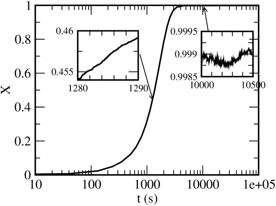
Figure 1: Crystalline fraction $X$ as a function of time during low temperature anneals at $131^{o}C$. Detail of the progress of the anneal is shown during the growth phase and when the crystalline fraction has saturated near $X=1$.

   

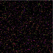
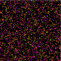
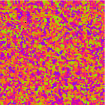
(a)                                   (b)                                   (c)

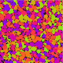
(d)

Figure 2: Images showing progress in crystallisation (a-c) for $T=131^{o}C$ (as shown in Figure 1); and (d) for $T=407^{o}C$, starting with pure amorphous material. The colours are assigned arbitrarily to different oriented crystal grains. (a) shows after 2000 steps of the algorithm a number of nuclei with $X=0.0507$ after time $248s$, (b) shows after $10000$ steps with $X=0.204$ after time $743s$, (c) shows after $10^{5}$ steps with $X=0.999115$ after time $68930s$. Similarly, (d) shows the state after $10^{6}$ steps corresponding to $4.347\mu s$ at the higher temperature. Observe the faster progress and larger crystals that result at the higher temperature.

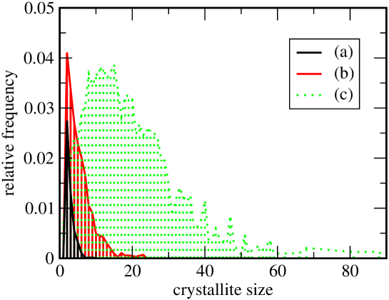
Figure 3: The relative frequency of crystallites of different sizes corresponding to the (a), (b) and (c) of Figure 2. Observe the peak in crystal size distribution at size 15-20 for the developed crystal structure (c).

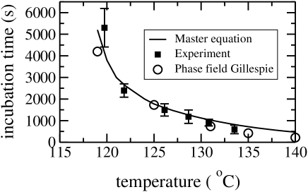
Figure 4: Incubation times given by Phase Field Gillespie simulations, with master equation simulations of GST crystallisation from BABW_2005 and experimental data from WFZW shown for comparison. Note that the Phase Field Gillespie simulation produces an excellent agreement with experiment.

 

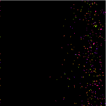
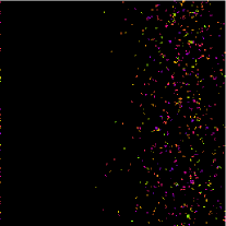
(a)                                   (b)

 

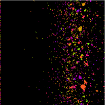
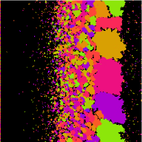
(c)                                   (d)

Figure 5: Images showing progress in crystallisation for a sample held in a temperature gradient where the left boundary is $227^{o}C$ and the right is $477^{o}C$. Observe the appearence of a band of higher crystallinity as time progresses from (a) after $17.6ns$, (b) after $70ns$, (c) after $554ns$ and (d) after $22.9\mu s$. Observe that the effective nucleation size is larger on the right (hotter) side of the sample.

 

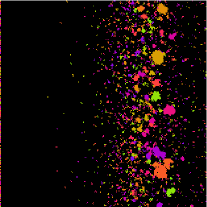
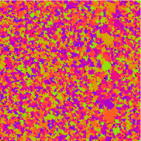
(a)                                   (b)

 

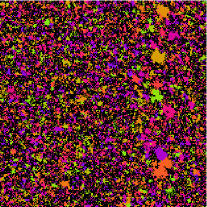
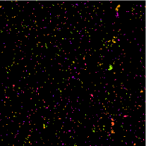
(c)                                   (d)

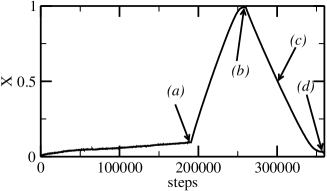
(e)

Figure 6: Progress of a multi-step anneal, demonstrating both spatial and temporal variation in temperatures. Starting from amorphous, a sample is first subjected $1\mu s$ of a linear spatial temperature gradient, the left at $227^{o}C$ and the right at $477^{o}C$; (a) shows resulting the crystal structure. For the next $0.1s$ it is maintained at $227^{o}C$ and in doing so progresses towards almost complete crystallisation but with a clear banded structure shown in (b). Finally the sample is raised to $477^{o}C$ for $15ns$ which is enough for the crystals to almost entirely dissociate; the structure at $X=0.5$ is shown in (c) and the final state is (d). Although below melting temperature, the critical nucleus size is too large for crystals of this size to survive. (e) Shows the crystalline fraction X as a function of algorithm step; the timesteps vary by many orders of magnitude as the anneal progresses.

References

- (1) K.B. Blyuss, P. Ashwin, A.P. Bassom and C.D. Wright. Master equation approach to the study of phase change processes in data storage media. Phys. Rev. E 72, 011607 (2005).
- (2) K.B. Blyuss, P. Ashwin, C.D. Wright and A.P. Bassom, Front propagation in a phase field model with phase-dependent heat absorption, Physica D 215, 127-136 (2006).
- (3) G. Caginalp and W. Xie, Phase-field and sharp-interface alloy models, Phys. Rev. E 48, 1897-1909 (1993).
- (4) D.T. Gillespie, Exact stochastic simulation of coupled chemical reactions, J. Phy. Chem., 81(25), 2340-2361 (1977).
- (5) D.T. Gillespie, Approximate accelerated stochastic simulation of chemically reacting systems J. Chem. Phys., 115, 1716-1733, (2001).
- (6) B. Hyot, V. Gehanno, B. Rolland, A. Fargeix, C. Vannufel, F. Charlet, B. Béchevet, J.M. Bruneau and P.J. Desre, Amorphization and Crystallization Mechanisms in GeSbTe-Based Phase Change Optical Disks J. Magn. Soc. Japan 25, 414 (2001).
- (7) A. Karma and W.-J. Rappel, Qualitative phase-field modeling of dendritic growth in two and three dimensions, Phys. Rev. E 57, 4323-4349 (1998).
- (8) D. Kashchiev, Nucleation (Butterworth-Heinemann, Oxford, 2000).
- (9) K.F. Kelton, A.L. Greer and C.V. Thompson, Transient nucleation in condensed systems J. Chem. Phys. 79, 6261 (1983).
- (10) Sung Soon Kim, Seong Min Jeong, Keun Ho Lee, Young Kwan Park, Young Tae Kim, Jeong Taek Kong and Hong Lim Lee, Simulation for Reset Operation of Phase-Change Random Access Memory Japanese J. Applied Physics 44, 5943-5948 (2005).
- (11) A.V. Kolobov, P. Fons, A.I. Frenkel, A.L. Ankudinov, J. Tominaga and T. Uruga, Understanding the phase-change mechanism of rewriteable optical media, Nature Mat., 3, 703-708 (2004).
- (12) S.R. Ovshinsky, Optical Cognitive Information Processing A New Field, Jap. J. App. Phys. 43, 4695 (2004).
- (13) S. Senkader and C.D. Wright, Models for phase-change in optical and electrical memory devices, J. App. Phy., 95, 504-511 (2004).
- (14) S. Vendantam and B.S.V.Patnaik, Efficient numerical algorithm for multiphase field simulations, Phy. Rev. E 73, E016703 (2006).
- (15) V. Weidenhof, I. Friedrich, S. Ziegler, M. Wuttig, Laser induced crystallization of amorphous film, J. Appl. Phys. 89, 3168-3176 (2001).
- (16) C. D. Wright, P. Ashwin and K. Blyuss. Master equation approach to understanding multi-state phase-change memories and processors, Applied Physics Letters 90, 063113 (2007).
- (17) N. Yamada, E. Ohno, K. Nishiuchi, N. Akahira and M. Takao, Rapid-phase transitions of pseudobinary amorphous thin films for an optical disk memory J. Appl. Phys. 69, 2849 (1991).
- (18) W. Yu, C.D. Wright, S.P. Banks and E.P. Palmiere, Cellular automata method for simulating microstructure evolution Science, Measurement and Technology, IEE Proceedings 150, 211 - 213 (2003).
(a) (b) (c)
(d)
(a) (b)
(c) (d)
(a) (b)
(c) (d)
(e)