Exact Solution of Semi-Flexible and Super-Flexible Interacting Partially Directed Walks

Abstract

We provide the exact generating function for semi-flexible and super-flexible interacting partially directed walks and also analyse the solution in detail. We demonstrate that while fully flexible walks have a collapse transition that is second order and obeys tricritical scaling, once positive stiffness is introduced the collapse transition becomes first order. This confirms a recent conjecture based on numerical results. We note that the addition of an horizontal force in either case does not affect the order of the transition. In the opposite case where stiffness is discouraged by the energy potential introduced, which we denote the super-flexible case, the transition also changes, though more subtly, with the crossover exponent remaining unmoved from the neutral case but the entropic exponents changing.

1 Introduction

The collapse transition of an isolated polymer has continued to attract both theoretical and experimental attention. The canonical lattice model of single polymer collapse has been the self-avoiding walk with the addition of attractive potentials between non-bonded nearest-neighbour sites of the walk. This is known as the Interacting Self-avoiding Walk (ISAW). This model has yielded many important theoretical aspects of the physical problem though it is not exactly solved in the sense that the generating function of partition functions has not been explicitly calculated, in two or three dimensions. An exactly solved version of the model does exist however when the restriction of partial directness is imposed on the configurations of the self-avoiding walk in two dimensions. The model has been shown to display a tricritical-like collapse transition [1] as is predicted for the unrestricted model, though with different exponents.

The Interacting Partially Directed Self-avoiding Walk (IPDSAW) model, and a closely related semi-continuous variant, on the square lattice was studied extensively in the early 1990’s [2, 3, 4, 5, 1, 6]. It was noticed that this problem is in a family of related problems including lattice models of vesicles [7, 8] whose solution can be written in terms of $q$-Bessel functions: moreover, direct correspondences occur between various models. Importantly, key work associated with the asymptotic analysis of the functions that arise in this class of problems was also completed [9]. Taken together these works completely solve and analyse the generating function, and free energy, of the IPDSAW model. In particular, the location of the collapse transition was found by Binder et al. [2] while the exact generating function was found by Brak et al. [3] in terms of $q$–Bessel functions. The tricritical nature of the collapse transition was elucidated by Owczarek et al. [1] and the full asymptotics of the generating function can be deduced from the work of Prellberg [9].

The addition of a stiffness parameter to mimic the effects of persistence length [10] and a stretching parameter to model the pulling of a polymer by an external force has more recently been studied in the context of the ISAW model [11]. While a parameter called a pulling force was not explicitly mentioned in the work on the IPDSAW it was implicitly part of the set up of the model, as we shall see below, since the horizontal and vertical steps of the walk were given separate fugacities. It was shown [1, 9] that differentiating the horizontal and vertical fugacities does not affect the nature of the collapse transition. Separate analysis of the IPDSAW model with the force interpretation being explicit confirms this [12]. On the other hand, the addition of a stiffness parameter so that the polymer is now semi-flexible was not included in the original definition of the model. The IPDSAW has recently been reconsidered by Zhou et al. [13]. Interestingly, they conjectured, on the basis of Monte Carlo simulation, and an approximation scheme allowing precise numerical estimates of thermodynamic quantities, of semi-stiff IPDSAW, that positive stiffness changes the order of the collapse transition to first-order. The three-dimensional semi-stiff ISAW model has been studied by Grassberger and Hegger [10] some time ago and they showed that the collapse transition does indeed become first order though only for a finite amount of applied stiffness. That is, small stiffness parameter values do not change the nature of the collapse transition. A related model shows similar behaviour [14]. In this paper we solve exactly the IPDSAW with stiffness parameter, which we shall now refer to as the Variably-Flexible Interacting Partially Directed Walk (VFIPDSAW) and analyse the model in the full parameter space. We show that not only does the collapse transition become first order when the stiffness parameter is positive (semi-flexible case) but it is also modified, though still tricritical, when the stiffness parameter is negative (super-flexible case).

1.1 The model

Consider the square lattice and a self-avoiding walk that has one end fixed at the origin on that lattice. Now restrict the configurations considered to self-avoiding walks such that starting at the origin only steps in the $(1,0)$, $(0,1)$ and $(0,-1)$ are permitted: such a walk is known as a Partially Directed Self-avoiding Walk (PDSAW). For convenience, we consider walks that have at least one horizontal step. Let the total number of steps in the walk be $L$ and the number of horizontal steps be $N$. Hence, we have $L\geq N\geq 1$. An example configuration along with the associated variables of our model are illustrated in Figure 1.

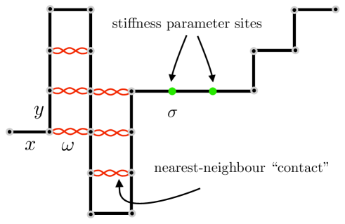
Figure 1: An example of a Partially Directed Walk of length $L=21$ and horizontal length $N=8$ (the bold black path) with the four parameters $x$ associated with horizontal steps, $y$ associated with vertical steps, $\omega$ associated with nearest-neighbour ‘contacts’ (shown as (red) intertwined curves) and the stiffness parameter $\sigma$ associated with the sites (highlighted in grey (green)) between two consecutive horizontal steps . The weight of the configuration shown is $x^{8}y^{13}\omega^{6}\sigma^{2}$.

We begin by recalling the definition of the IPDSAW model and then add the “stiffness parameter”, the addition of which defines our model.

IPDSAW

To define the IPDSAW model we add various energies to properties of this walk and hence Boltzmann weights to the walk. Firstly, any two occupied sites of the walk not adjacent in the walk though adjacent on the lattice are denoted “nearest-neighbour contacts”: see Figure 1. An energy $-J$ is added for each such contact. We define a Boltzmann weight $\omega=e^{\beta J}$ associated with these contacts, where $\beta=1/k_{B}T$ and $T$ is the absolute temperature. An external horizontal force $f$ pulling at the other end of the walk adds a Boltzmann weight $p^{N}$ and $p=e^{\beta fa_{0}}$, with $a_{0}$ being the length of a lattice bond. The partition function $Z^{\mathrm{IPDSAW}}_{L}(\omega,p)$ of the IPDSAW model is

$$Z^{\mathrm{IPDSAW}}_{L}(\omega,p)=\sum_{\mathrm{PDSAW\;of\;length\;}L}\omega^{m}p^{N}\,,$$ (1.1)

where $m$ is the number of nearest-neighbour contacts in the PDSAW. The generating function $\hat{G}^{\mathrm{IPDSAW}}(z,\omega,p)$

$$\hat{G}^{\mathrm{IPDSAW}}(z,\omega,p)=\sum_{L=1}^{\infty}Z^{IPDSAW}_{L}(\omega,p)z^{L}\,,$$ (1.2)

so $z$ can be considered as fugacity for the steps of the walk and the generating function a “generalised partition function” [1]. In previous work [1] an alternate generating function $G^{IPDSAW}(x,y,\omega)$ was considered, where instead of a force parameter $p$ horizontal steps were weighted with a fugacity $x$ while vertical steps were given a fugacity $y$: see Figure 1. Hence we have

$$\hat{G}^{\mathrm{IPDSAW}}(z,\omega,p)=G^{\mathrm{IPDSAW}}(pz,z,\omega)\,.$$ (1.3)

Clearly considering a separate horizontal fugacity is equivalent to considering a horizontal pulling force at the level of generating functions.

VFIPDSAW

To define the VFIPDSAW we now add an energy $-\Delta$ to each site between consecutive horizontal steps of the walk: see figure 1. Note that for $\Delta>0$ consecutive horizontal steps are favoured and so this is the positive stiffness, or semi-flexible, regime while for $\Delta<0$ consecutive horizontal steps are discouraged so this is the negative stiffness, or super-flexible regime. If $\ell$ is the number of such “stiffness” sites in a particular IPDSAW then such a configuration is associated with an additional Boltzmann factor $\sigma^{\ell}$ where $\sigma=e^{\beta\Delta}$. That is, each configuration has weight $\omega^{m}p^{N}\sigma^{\ell}$. Note that one could have equivalently chosen to weight every bend, or change of direction of the walk, with a weight $b$ say. That is, each configuration has weight $\omega^{m}p^{N}b^{k}$. However, since the number of such bends $k$ is related to the number of horizontal straight segments, $\ell$, assuming for convenience at least one vertical step in the walk, as

$$\ell=\frac{(2N-k-1)}{2}\,,$$ (1.4)

then substituting $\sigma=1/b^{2}$ and setting $p$ to $pb^{2}$ gives the same weight for each configuration (barring an overall factor of $b$).

The partition function for VFIPDSAW is defined as

$$Z^{\mathrm{VFIPDSAW}}_{L}(\omega,p,\sigma)=\sum_{\mathrm{PDSAW\;of\;length\;}L}\omega^{m}p^{N}\sigma^{\ell}\,,$$ (1.5)

while the generating function, analogously to the fully-flexible case above, $G^{\mathrm{VFIPDSAW}}(x,y,\omega,\sigma)$, is given as

$$G^{\mathrm{VFIPDSAW}}(pz,z,\omega,\sigma)=\sum_{L=1}^{\infty}Z^{\mathrm{VFIPDSAW}}_{L}(\omega,p,\sigma)z^{L}\,.$$ (1.6)

Clearly one can recover the fully flexible case by setting $\sigma=1$:

$$G^{\mathrm{IPDSAW}}(pz,z,\omega)=G^{\mathrm{VFIPDSAW}}(pz,z,\omega,1)\,.$$ (1.7)

Setup

As we consider the VFIPDSAW model from now on we shall drop the superscript VFIPDSAW. The singularity structure of the generating function as function of $z$ determines the free energy. The reduced free energy is defined as

$$\kappa(\omega,p,\sigma)=-\lim_{L\rightarrow\infty}\frac{1}{L}\log\left[Z_{L}(\omega,p,\sigma)\right]$$ (1.8)

and is given by

$$\kappa(\omega,p,\sigma)=\log z_{s}(\omega,p,\sigma)\,,$$ (1.9)

where $z_{s}(\omega,p,\sigma)$ is the closest singularity (on the positive real axis) of the generating function $G(pz,z,\omega,\sigma)$ in the variable $z$ to the origin. Note also that

$$Z_{L}(\omega,p,\sigma)=[z^{L}]G(pz,z,\omega,\sigma)={\frac{1}{2}\pi i}\oint G(pz,z,\omega,\sigma){\frac{dz}{z^{L+1}}}.$$ (1.10)

In order to find the generating function it is advantageous to rewrite it in the following way. We can describe the PDSAW configurations in a natural way through the length $r_{i}$ of vertical segments between two horizontal steps, measured in the positive $y$–direction. Each PDSAW begins with a vertical segment of height $r_{1}$ followed by an horizontal step. Thus, we associate to each configuration an $N$–tuple $(r_{1},r_{2},\ldots,r_{N})$ corresponding to a configuration of total length $L=\sum_{i=1}^{N}|r_{i}|+N$. The energy due to the nearest–neighbour contacts for each of these configurations is then

$$-J\;u(r_{1},r_{2},\ldots,r_{N})\,,$$ (1.11)

where

$$u(r_{1},r_{2},\ldots,r_{N})=\sum_{i=1}^{N-1}\min(|r_{i}|,|r_{i+1}|){\Theta}(-r_{i}r_{i+1})\,,$$ (1.12)

where $\Theta(r)$ is the Heaviside step function:

$${\Theta}(r)=\left\{\begin{array}[]{cl}0&r<0,\\ 1/2&r=0,\\ 1&r>0.\end{array}\right.\\$$ (1.13)

The number of “stiffness sites” $\ell$ is then given by the number of times $r_{i}=0$ for any $1<i\leq N$.

We get the generating function by summing over all possible lengths as

$$G(x,y,\omega,\sigma)=\sum_{L=1}^{\infty}\sum_{N=1}^{L}x^{N}\sum_{|r_{1}|+|r_{2}|+\ldots+|r_{N}|=L-N}y^{L-N}\omega^{u(r_{1},r_{2},\ldots,r_{N})}\sigma^{\ell}\,,$$ (1.14)

that is,

$$G(x,y,\omega,\sigma)=\sum_{N=1}^{\infty}x^{N}\sum_{M=0}^{\infty}y^{M}\sum_{|r_{1}|+|r_{2}|+\ldots+|r_{N}|=M}\omega^{u(r_{1},r_{2},\ldots,r_{N})}\sigma^{\ell}\,.$$ (1.15)

2 Exact solution of the generating function

In order to derive an expression for $G(x,y,\omega,\sigma)$, consider the generalised partition functions $G_{r}=G_{r}(x,y,\omega,\sigma)$ for walks that start with a vertical segment of height $r$, so that

$$G(x,y,\omega,\sigma)=\sum_{r\in\mathbb{Z}}G_{r}.$$ (2.1)

Then we can concatenate these walks to get a recursion relation for $G_{r}$ as follows:

$$G_{r}=xy^{|r|}\left\{1+\sigma^{\delta_{r,0}}G_{0}+\sum_{s\in\mathbb{Z}\setminus\{0\}}\omega^{u(r,s)}G_{s}\right\}\,.$$ (2.2)

It follows that

$$G_{0}=x\left\{1+(\sigma-1)G_{0}+G\right\}\,,$$ (2.3)

so that

$$G_{0}=xu\left\{1+G\right\}\,,$$ (2.4)

where

$$u=\frac{1}{1-x(\sigma-1)}.$$ (2.5)

Using the symmetry $G_{r}=G_{-r}$ and then restricting to $r\geq 0$, we can further simplify to

$$G_{r}=xy^{r}\left\{1+\sigma^{\delta_{r,0}}G_{0}+\sum_{s=1}^{\infty}(1+\omega^{\min(r,s)})G_{s}\right\}\,,$$ (2.6)

which will be the starting point of our investigation. Since $r=0$ is now special we will need to consider $r=1$ separately also:

$$G_{1}=xy\left\{1+G_{0}+(1+\omega)\sum_{s=1}^{\infty}G_{s}\right\}\,.$$ (2.7)

Now using

$$\sum_{s=1}^{\infty}G_{s}=\frac{1}{2}(G-G_{0})$$ (2.8)

gives

$$G_{1}=xy\left\{1+\frac{(1-\omega)}{2}G_{0}+\frac{(1+\omega)}{2}G\right\}\,.$$ (2.9)

Now using equation (2.4) we obtain

$$G_{1}=xy\left\{\frac{(1-\omega)}{2}+\left(\frac{(1+\omega)}{2}+\frac{(1-\omega)}{2}xu\right)(1+G)\right\}\,.$$ (2.10)

Hence the ratio $G_{1}/G_{0}$ can be written in terms of $1+G$. By solving for $(1+G)$ one finds

$$1+G=\frac{(1-\omega)}{2}\left[\frac{uG_{1}}{yG_{0}}-\left(\frac{(1+\omega)}{2}+\frac{(1-\omega)}{2}xu\right)\right]^{-1}\,.$$ (2.11)

We will now derive a homogeneous second order difference equation which we can solve using the same ansatz used previously [1]. Using the scaling behaviour of the solutions, we can eliminate one of the two linearly independent solutions. We then write the general solution of (2.6) as an expression involving the quotient of two $q$–hypergeometric functions.

Taking differences in (2.6), we first eliminate the inhomogeneous term,

$$G_{r+1}-yG_{r}=\delta_{r,0}xy(1-\sigma)G_{0}+xq^{r+1}(1-\frac{1}{\omega})\sum_{s=r+1}^{\infty}G_{s}.$$ (2.12)

Here, we introduced for convenience the new variable $q=y\omega$. Upon taking differences a second time, we are left with

$$(G_{r+2}-yG_{r+1})-q(G_{r+1}-yG_{r})=-\delta_{r,0}qxy(1-\sigma)G_{0}-xq^{r+2}(1-\frac{1}{\omega})G_{r+1}.$$ (2.13)

We now solve this equation for $r\geq 1$ and subsequently solve for $r=0$. In the case of no interaction ($\omega=1$), the right hand side of this equation is zero (for $r\geq 1$) and we have a simple homogeneous difference equation with constant coefficients. Its characteristic polynomial $P(\lambda)$ is

$$P(\lambda)=(\lambda-y)(\lambda-q)$$ (2.14)

and the solution is given by $G_{r}=A_{1}y^{r}+A_{2}q^{r}$.

This motivates the ansatz [15]

$$G_{r}=\lambda^{r}\sum_{n=0}^{\infty}q^{nr}c_{n}\,,$$ (2.15)

with $c_{n}=c_{n}(x,q,\omega)$ independent of $r\geq 1$, which inserted into (2.13) gives

$$P(\lambda)c_{0}+\sum_{n=1}^{\infty}q^{nr}\left(P(\lambda q^{n})c_{n}+xq(1-\frac{1}{\omega})\lambda q^{n}c_{n-1}\right)=0.$$ (2.16)

This equation is solved by

$$P(\lambda)=0,\quad\mbox{i.e.}\quad\lambda_{1}=y\quad\mbox{and}\quad\lambda_{2}=q,$$ (2.17)

and, choosing $c_{0}=1$,

$$c_{n}=\prod_{m=1}^{n}\frac{-xq(1-\frac{1}{\omega})\lambda q^{m}}{P(\lambda q^{m})}=\frac{\left(-x\omega(1-\frac{1}{\omega})\lambda\right)^{n}q^{\binom{n}{2}}}{(\lambda\omega;q)_{n}(\lambda;q)_{n}}.$$ (2.18)

Here we have used the standard notation

$$(x;q)_{n}=\prod_{m=1}^{n}(1-xq^{m-1}).$$ (2.19)

Defining

$$H(y,q,t)=\sum_{n=0}^{\infty}\frac{q^{\binom{n}{2}}(-t)^{n}}{(y;q)_{n}(q;q)_{n}}\,,$$ (2.20)

we now can write the general solution of (2.13), for $r\geq 1$, as

$$G_{r}=A_{1}y^{r}H(y,q,x(1-\frac{1}{\omega})q^{1+r})+A_{2}q^{r}H(q\omega,q,x\omega(1-\frac{1}{\omega})q^{1+r}).$$ (2.21)

We remark that the function $H$ is directly related to a basic hypergeometric function [16]

$$H(y,q,t)={}_{1}\phi_{1}(0,y;q,t)\,,$$ (2.22)

which can be seen to be a limiting function of ${}_{2}\phi_{1}$ and that is the $q$–deformation of the more familiar hypergeometric function ${}_{2}F_{1}$. Analogously, the function $H$ can be understood (apart from some normalising factors and seen by taking the limit $q\rightarrow 1$) as a $q$–generalisation of Bessel functions. One can easily verify that $H(y,q,t)$ satisfies the following recurrence

$$qH(y,q,t)+(tq-(y+q))H(y,q,qt)+yH(y,q,q^{2}t)=0\,.$$ (2.23)

Returning to the analysis we see that, for $|q|<1$, $H(y,q,tq^{r})$ is uniformly bounded in $r$, so that we can write

$$|G_{r}|\leq\mbox{const\ }(q^{r}+y^{r}).$$ (2.24)

This we insert into (2.6) and, assuming $0<\omega^{2}y<1<\omega$ we get

$$|G_{r}| \leq \mbox{const\ }y^{r}\left(1+\sum_{s=0}^{r-1}(\omega q)^{s}+\omega^{r}\sum_{s=r}^{\infty}q^{s}\right)$$ (2.26)

$$\leq \mbox{const\ }y^{r}(1+(\omega q)^{r})\leq\mbox{const\ }y^{r}.$$

As $H(y,q,tq^{r})\rightarrow 1$ for $r\rightarrow\infty$, we see that in fact $A_{2}=0$. The reason for this is that we obtained the homogeneous difference equation (2.13) by taking differences from (2.6), thus introducing additional solutions.

We now note that the ratios $G_{r+1}/G_{r}$ contain no unknown constants. In fact, defining

$${\cal H}(y,q,t)=\frac{H(y,q,qt)}{H(y,q,t)}\,,$$ (2.27)

we find

$$\frac{G_{r+1}}{yG_{r}}={\cal H}(y,q,x(1-\frac{1}{\omega})q^{1+r})\qquad\text{for $r\geq 1$.}$$ (2.28)

Note in passing that successive ratios are related via the following recurrence for ${\cal H}(y,q,t)$ derived from equation (2.23),

$${\cal H}(y,q,t)=q\left[y+q-tq-y{\cal H}(y,q,qt)\right]^{-1}\;.$$ (2.29)

In fact, the ratio $G_{1}/G_{0}$ is given by a very similar expression. For $r=0$, the recursion (2.13) can be rewritten as

$$(G_{2}-yG_{1})-q(G_{1}-\frac{y}{u}G_{0})=-xq^{2}(1-\frac{1}{\omega})G_{1}\;,$$ (2.30)

from whence one can conclude that

$$\frac{uG_{1}}{yG_{0}}={\cal H}(y,q,x(1-\frac{1}{\omega})q)\;.$$ (2.31)

Inserting this ratio into equation (2.11) and substituting $q=y\omega$, we have

$$1+G=\frac{(1-\omega)}{2}\left[{\cal H}(y,y\omega,x(\omega-1)y)-\left(\frac{(1+\omega)}{2}+\frac{(1-\omega)}{2}xu\right)\right]^{-1}\,.$$ (2.32)

We note immediately that the stiffness parameter $\sigma$ only enters (via $u$) in one term of this expression. For $\sigma=1$ (i.e. $u=1$), this is exactly equation (4.27) in [1].

Our final expression for the solution of the generating function for the Variably Flexible Interacting Partially Directed Walk in the variables $z,\omega,p,\sigma$ is therefore

$$1+G=\frac{(1-\omega)}{2}\left[{\cal H}(z,z\omega,pz^{2}(\omega-1))-\left(\frac{(1+\omega)}{2}+\frac{(1-\omega)}{2}\frac{pz}{1-pz(\sigma-1)}\right)\right]^{-1}\,.$$ (2.33)

As we will see below the case $q=1$ is important. From (2.29) it follows that ${\cal H}(y,1,t)$ is the root of a quadratic equation, and so

$${\cal H}(y,1,t)=\frac{1}{2y}\left[1+y-t-\sqrt{(1+y-t)^{2}-4y}\right]\;,$$ (2.34)

where the branch has been chosen such that ${\cal H}(y,1,t)=1+O(t)$. There is an algebraic singularity at $(1+t-y)^{2}=4y$ and the solution is real-valued as long as $(1+t-y)^{2}\geq 4y$.

One can therefore solve for the generating function along the curve $y\omega=1$ as

$$1+G=\frac{(1-\omega)}{2}\left[{\cal H}(\frac{1}{\omega},1,x(1-\frac{1}{\omega}))-\left(\frac{(1+\omega)}{2}+\frac{(1-\omega)}{2}xu\right)\right]^{-1}\,.$$ (2.35)

which is now algebraic.

3 Analysis of the Phase diagram

3.1 General considerations

One can immediately observe that the generating function $G$ has singularities at the singularities of ${\cal H}(y,y\omega,x(\omega-1)y)$ and when the denominator is zero, that is, at solutions $\omega_{c}(x,y,u)$ of

$${\cal H}(y,y\omega,x(\omega-1)y)=\left(\frac{(1+\omega)}{2}+\frac{(1-\omega)}{2}xu\right)\,.$$ (3.1)

There is an essential singularity of ${\cal H}(y,y\omega,x(1-\omega)y)$ when $y\omega=1$. On the other hand, when the denominator is zero, $G$ has a pole, and the locus $\omega_{c}(x,y,u)$ of this pole depends analytically on the parameters as long as $y\omega<1$. If there is no zero of the denominator for $y\omega<1$, then the closest singularity is given by the essential singularity of ${\cal H}(y,y\omega,x(1-\omega)y)$ at $y\omega=1$ where the generating function converges. On this curve, we obtain from (2.35) that there is an algebraic singularity at

$$\omega_{a}(x)=\left(\frac{1+x}{1-x}\right)^{2}$$ (3.2)

and for $u>1$ a simple pole at

$$\omega_{p}(x,u)=\frac{(1+ux)(1+2x-ux)}{(1-ux)(1-2x+ux)}\;.$$ (3.3)

These singularities coincide when $u=1$, at which value the nature of the algebraic singularity changes. Note that for $u<1$ the pole disappears.

As stated above for any fixed $\omega$ the generating function as a function of $y$ either has a pole given by the solution of $\omega=\omega_{c}(x,y,u)$ or has a singularity on the curve $y=1/\omega$. Therefore, for $u\leq 1$, $\omega_{c}(x,y,u)$ meets the algebraic singularity $\omega_{a}(x)$ as the curve $y\omega=1$ is approached, whereas for $u>1$, $\omega_{c}(x,y,u)$ meets the pole $\omega_{p}(x,u)$ as the curve $y\omega=1$ is approached. To investigate the behaviour of $G$ near the curve $y\omega=1$ more closely, we need the asymptotic behaviour of ${\cal H}(y,q,t)$ as $q\rightarrow 1$. Away from the algebraic singularity, i.e. for $(1+t-y)^{2}>4y$, we can use (2.29) to derive an asymptotic expansion in $\epsilon=1-q$,

$${\cal H}(y,1-\epsilon,t)\sim\sum_{n=0}^{\infty}{\cal H}^{(n)}(y,t)\epsilon^{n}$$ (3.4)

with the first terms given by ${\cal H}^{(0)}(y,t)={\cal H}(y,1,t)$ and

$${\cal H}^{(1)}(y,t)= \frac{{\cal H}^{(0)}(y,t)}{y{\cal H}^{(0)}(y,t)^{2}-1}\left[1+yt{\cal H}^{(0)}(y,t)\frac{\partial}{\partial t}{\cal H}^{(0)}(y,t)+(t-1){\cal H}^{(0)}(y,t)\right]$$ (3.5)

$$= -\frac{1}{2y}\left(1+\frac{y+t-1}{\sqrt{(1+y-t)^{2}-4y}}+\frac{2yt}{(1+y-t)^{2}-4y}\right)\;.$$ (3.6)

Close to the algebraic singularity at $q=1$, the singularity structure is significantly more complicated, but has been thoroughly elucidated in [9]. Using Lemma 4.3 from [9], a result completely analogous to Theorem 5.3 in [9] can be obtained for ${\cal H}(x,q,t)$, i.e. an asymptotic expansion in $q=1-\epsilon$ uniformly valid for all values of $t$ and $x$, which reads

$${\cal H}(y,1-\epsilon,t)=\frac{1}{2y}\left[1+y-t-\left(-\frac{\operatorname{Ai}^{\prime}(\alpha\epsilon^{-2/3})}{\alpha^{1/2}\epsilon^{-1/3}\operatorname{Ai}(\alpha\epsilon^{-2/3})}\right)\sqrt{(1+y-t)^{2}-4y}\right](1+O(\epsilon))\;.$$ (3.7)

Note that for $\epsilon\rightarrow 0$ the expression multiplying the square root in (3.7) tends to $1$ as is necessary. Here, $\alpha=\alpha(y,t)$ is a function of $y$ and $t$ which is known exactly [9]. While the precise form of $\alpha$ is rather cumbersome, it simplifies considerably near the critical point, and we find

$$\alpha(y,t)\sim\left(\frac{4}{1-(t-y)^{2}}\right)^{4/3}\frac{(1+y-t)^{2}-4y}{4}$$ (3.8)

for small $(1+y-t)^{2}-4y$. This implies that here

$${\cal H}(y,1-\epsilon,t)\sim\frac{1}{2y}\left[1+y-t+\epsilon^{1/3}\frac{\operatorname{Ai}^{\prime}(\alpha\epsilon^{-2/3})}{\operatorname{Ai}(\alpha\epsilon^{-2/3})}\frac{(1-(t-y)^{2})^{2/3}}{2^{1/3}}\right]\;.$$ (3.9)

The behaviour of this expression is determined by the function $f(z)=-\operatorname{Ai}^{\prime}(z)/\operatorname{Ai}(z)$, the graph of which is shown in figure 2. The large-$z$ asymptotics allows for matching for $\epsilon\rightarrow 0$ and positive $\alpha$. For negative $\alpha$, the argument of $f$ is negative. As $f(z)$ has a simple pole at $z=-2.3381\ldots$, for any fixed $\alpha<0$ we have a pole at a finite value of $\epsilon$. As $\alpha$ tends to zero, the locus of this pole scales as $\epsilon^{2/3}$.

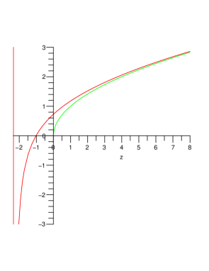
Figure 2: The graph of $f(z)=-\operatorname{Ai}^{\prime}(z)/\operatorname{Ai}(z)$. The function $f$ has a simple pole at $z=-2.3381\ldots$, a zero at $z=-1.0187\ldots$, and is asymptotic to $\sqrt{z}$ for large $z$, which is plotted for comparison.

3.2 Fully flexible case ($\Delta=0$)

This case is the one considered in our earlier work [1]. Here $u=1$, and the simple pole at $\omega_{c}(x,y,1)$ approaches an algebraic singularity at $\omega_{t}=\left(\frac{1+x}{1-x}\right)^{2}>1$, at which the generating function diverges. In particular, we find

$$1+G\sim\left(-\frac{\operatorname{Ai}^{\prime}(\alpha\epsilon^{-2/3})}{\alpha^{1/2}\epsilon^{-1/3}\operatorname{Ai}(\alpha\epsilon^{-2/3})}\right)^{-1}\frac{\omega-1}{\sqrt{(1+\omega+x(1-\omega))^{2}-4\omega}}$$ (3.10)

as $\epsilon=1-y\omega\rightarrow 0$, with $\alpha=\alpha(\frac{1}{\omega},x(1-\frac{1}{\omega}))$ given by (3.8). Near the transition, $\alpha$ is small and we can write

$$1+G\sim -A\epsilon^{-1/3}\frac{\operatorname{Ai}(\alpha\epsilon^{-2/3})}{\operatorname{Ai}^{\prime}(\alpha\epsilon^{-2/3})}$$ (3.11)

with $A=(\omega-1)/[\omega^{2}-(x(\omega-1)-1)^{2}]^{2/3}(2\omega)^{1/3}$. For $\omega=\omega_{t}$, $\alpha=0$ and $G$ diverges as $\epsilon^{-1/3}$. For $\omega>\omega_{t}$, $\alpha>0$ and $G$ tends to a finite value given by (2.35). For $\omega<\omega_{t}$, $\alpha<0$ and $G$ has a simple pole at $\alpha\epsilon^{2/3}\approx-1.0187\ldots$. We accordingly have a second-order phase transition characterised by

$$\gamma_{u}=\frac{1}{2}\qquad\gamma_{t}=\frac{1}{3}\qquad\phi=\frac{2}{3}\;,$$ (3.12)

with the exponents as defined by Owczarek et al. [1].

Changing to the variables $z,\omega,p,\sigma$ this can be formulated as follows. This is the case $\sigma=1$, and there is a curve of simple poles given by $\omega_{c}(pz,z,1)$ approaching the curve $\omega z=1$ at $\omega_{t}$ given by $\omega_{t}=\left(\frac{p+\omega_{t}}{p-\omega_{t}}\right)^{2}$. For $p=1$, the solution is $\omega_{t}=3.3829\ldots$. Near the transition, (3.10) holds with the appropriate substitution $x=pz$ and $y=z$. While the location $\omega_{c}(pz,z,1)$ of the poles, as well as $\omega_{t}$ change as a function of $p$, the character of the phase transition does not.

3.3 Super-flexible case ($\Delta<0$)

Now $u<1$, and the simple pole at $\omega_{c}(x,y,u)$ approaches an algebraic singularity at $\omega_{t}=\left(\frac{1+x}{1-x}\right)^{2}>1$, at which the generating function converges. In particular, we find

$$1+G\sim \frac{\omega-1}{x(\omega-1)(1-u)+\left(-\frac{\operatorname{Ai}^{\prime}(\alpha\epsilon^{-2/3})}{\alpha^{1/2}\epsilon^{-1/3}\operatorname{Ai}(\alpha\epsilon^{-2/3})}\right)\sqrt{(1+\omega+x(1-\omega))^{2}-4\omega}}$$ (3.13)

as $\epsilon=1-y\omega\rightarrow 0$, with $\alpha=\alpha(\frac{1}{\omega},x(1-\frac{1}{\omega}))$ given by (3.8). Near the transition, $\alpha$ is small and we can write

$$1+G\sim \frac{1}{x(1-u)-A^{-1}\epsilon^{1/3}\frac{\operatorname{Ai}^{\prime}(\alpha\epsilon^{-2/3})}{\operatorname{Ai}(\alpha\epsilon^{-2/3})}}$$ (3.14)

with $A$ as above. For $\omega=\omega_{t}$, $\alpha=0$ and $G$ converges with the singular part scaling as $\epsilon^{1/3}$. For $\omega>\omega_{t}$, $\alpha>0$ and $G$ tends to a finite value given by (2.35). For $\omega<\omega_{t}$, $\alpha<0$ and $G$ has a simple pole at some value of $\epsilon$ where $-\operatorname{Ai}^{\prime}(z)/\operatorname{Ai}(z)<0$, i.e. $-2.3381\ldots<\alpha\epsilon^{2/3}<-1.0187\ldots$. We now find a second-order phase transition with

$$\gamma_{u}=-\frac{1}{2}\qquad\gamma_{t}=-\frac{1}{3}\qquad\phi=\frac{2}{3}\;.$$ (3.15)

As $u\rightarrow 1$, we recover the fully flexible case discussed above.

Changing to the variables $z,\omega,p,\sigma$ this can be formulated as follows. This is the case $\sigma<1$, and there is a curve of simple poles given by $\omega_{c}(pz,z,(1-pz(\sigma-1))^{-1})$ approaching the curve $\omega z=1$ at $\omega_{t}$ given by $\omega_{t}=\left(\frac{p+\omega_{t}}{p-\omega_{t}}\right)^{2}$. This transition point therefore is independent of the value of $\sigma$, and is identical to the one obtained in the fully flexible case. Near the transition, (3.13) holds with the appropriate substitution $x=pz$, $y=z$, and $u=1/(1-pz(\sigma-1))$. While the location $\omega_{c}(pz,z,(1-pz(\sigma-1))^{-1})$ of the poles, as well as $\omega_{t}$ change as a function of $p$, the character of the phase transition does not.

3.4 Semi-flexible case ($\Delta>0$)

Now $u>1$, and the simple pole at $\omega_{c}(x,y,u)$ approaches a simple pole at $\omega_{t}=\frac{(1+ux)(1+2x-ux)}{(1-ux)(1-2x+ux)}>1$. In particular, we find near the transition that

$$1+G\sim\frac{\omega-1}{x(\omega-1)(1-u)+\sqrt{(1+\omega+x(1-\omega))^{2}-4\omega}-2\epsilon{\cal H}^{(1)}(\frac{1}{\omega},x(\omega-1)\frac{1}{\omega})}$$ (3.16)

as $\epsilon=1-y\omega\rightarrow 0$, with ${\cal H}^{(1)}$ given by (3.5). Note that $x(\omega-1)(1-u)+\sqrt{(1+\omega+x(1-\omega))^{2}-4\omega}$ is asymptotically linear in $\omega-\omega_{t}$ and is negative for $\omega<\omega_{t}$. Note further that ${\cal H}^{(1)}<0$. For $\omega>\omega_{t}$, $G$ tends to a finite value as $\epsilon\rightarrow 0$. This expression diverges with a simple pole as $\omega$ approaches $\omega_{t}$. Similarly, for $\omega=\omega_{t}$, $G$ diverges as $\epsilon^{-1}$. For $\omega<\omega_{t}$, $G$ has a simple pole at

$$\epsilon=\frac{x(\omega-1)(1-u)+\sqrt{(1+\omega+x(1-\omega))^{2}-4\omega}}{2{\cal H}^{(1)}(\frac{1}{\omega},x(\omega-1)\frac{1}{\omega})}\;.$$ (3.17)

We accordingly find a first-order phase transition with

$$\gamma_{u}=1\qquad\gamma_{t}=1\qquad\phi=1\;.$$ (3.18)

As $u\rightarrow 1$, ${\cal H}^{(1)}$ diverges, and the character of the phase transition changes as characterised above.

Changing to the variables $z,\omega,p,\sigma$ this can be formulated as follows. This is the case $\sigma>1$, and there is a curve of simple poles given by $\omega_{c}(pz,z,(1-pz(\sigma-1))^{-1})$ approaching the curve $\omega z=1$ at $\omega_{t}$ given by

$$\omega_{t}=\frac{(2(1-\sigma)p^{2}+(2-\sigma)\omega_{t}p+\omega_{t}^{2})((2-\sigma)p+\omega_{t})}{(2(\sigma-1)p^{2}-\omega_{t}p\sigma+\omega_{t}^{2})(\omega_{t}-p\sigma)}\;.$$ (3.19)

While this is quite cumbersome in general, some special values have simple solutions. For example, at $p=1$ and $\sigma=2$ we find $\omega_{t}=2+\sqrt{2}=3.4142\ldots$. Near the transition, (3.16) holds with the appropriate substitution $x=pz$, $y=z$, and $u=1/(1-pz(\sigma-1))$. While the location $\omega_{c}(pz,z,(1-pz(\sigma-1))^{-1})$ of the poles, as well as $\omega_{t}$ change as a function of $p$, the character of the phase transition does not.

4 Conclusion

We have analysed the exact solution of a two-dimensional lattice model of a single polymer in solution containing parameters that vary the intra-polymer attraction, the amount of horizontal stretching force applied and the amount of stiffness. The restriction of partial directness is required to ensure solvability. We find that a tricritical collapse transition takes place for no stiffness or negative stiffness, and that this is unaffected by an horizontal force. The entropic exponents are different in the negative stiffness regime to those in the zero stiffness regime. On the other hand, when the polymer becomes semi-stiff the collapse transition immediately becomes first-order.

References

• [1] A.ย L. Owczarek, T.ย Prellberg, and R.ย Brak, J. Stat. Phys. 72, 737 (1993).
• [2] P.ย M. Binder, A.ย L. Owczarek, A.ย R. Veal, and J.ย M. Yeomans, J. Phys. A 23, L975 (1990).
• [3] R.ย Brak, A.ย J. Guttmann, and S.ย G. Whittington, J. Phys. A 25, 2437 (1992).
• [4] T.ย Prellberg, A.ย L. Owczarek, R.ย Brak, and A.ย J. Guttmann, Phys. Rev. E. 48, 2386 (1993).
• [5] A.ย L. Owczarek, J. Phys. A. 26, L647 (1993).
• [6] A.ย L. Owczarek and T.ย Prellberg, Physica A 205, 203 (1994).
• [7] R.ย Brak, A.ย L. Owczarek, and T.ย Prellberg, J. Stat. Phys. 76, 1101 (1994).
• [8] T.ย Prellberg and R.ย Brak, J. Stat. Phys. 78, 701 (1995).
• [9] T.ย Prellberg, J. Phys. A 28, 1289 (1995).
• [10] P.ย Grassberger and R.ย Hegger, J. Chem. Phys. 102, 6881 (1995).
• [11] P.ย Grassberger and H.ย Hsu, Phys. Rev. E 65, 031807 (2002).
• [12] A.ย Rosa, D.ย Marenduzzo, A.ย Maritan, and F.ย Seno, Phys. Rev. E. 67, 041802 (2003).
• [13] H.ย Zhou, J.ย Zhou, Z.-C. Ou-Yang, and S.ย Kumar, Phys. Rev. Lett. 97, 158302 (2006).
• [14] J.ย Krawczyk, A.ย L. Owczarek, T.ย Prellberg, and A.ย Rechnitzer, The competition of hydrogen-like and isotropic interactions in polymer collapse, Stat. Mech.: Theor. Exp., 2007, In press.
• [15] V.ย Privman and N.ย M. ล vrakiฤ‡, Directed Models of Polymers, Interfaces, and Clusters: Scaling and Finiteโ€“Size Properties, volume 338 of Lecture Notes in Physics, Springerโ€“Verlag, Berlin, 1989.
• [16] G.ย Gasper and M.ย Rahman, Basic Hypergeometric Series, Camb. Univ., 1990.