Excitation and photoionization processes involving the bound $ns$ electrons

Abstract

We have considered the processes of excitation and ionization of light multicharged ions by impact of high-energy particles, which proceed with participation of the $ns$ electrons. The screening corrections to the energy levels and photoionization cross sections are evaluated analytically within the framework of the non-relativistic perturbation theory with respect to the electron-electron interaction. The universal scalings for the excitation and ionization cross sections are studied for arbitrary principal quantum numbers $n$.

1. Since decades the fundamental processes of excitation and ionization of few-electron atomic ions have been persistently investigated within the framework of different sophisticated approaches, due to necessity of the accurate account of all interactions in the colliding system (see, for example, the works 1 ; 2 ; 3 ; 4 ; 5 ; 6 ; 7 and references there). The deduction of the universal scaling behavior for differential and total cross sections is of particular importance, because it allows one to establish generic features of various processes for a wide family of targets 8 ; 9 ; 10 ; 11 . In this Letter, we study the excitation and photoionization of light multicharged ions, which proceed with participation of the $ns$ electrons. As a method, the consistent non-relativistic perturbation theory in the Furry picture is employed 12 . The calculations are performed analytically, taking into account the one-photon exchange diagrams.

The characteristic quantities for the theoretical description of collision processes on multicharged ions are the Coulomb potential $I=\eta^{2}/(2m)$ for single ionization from the K shell, the average momentum $\eta=m\alpha Z$ of the K-shell electron, the Bohr radius $a_{0}=1/(m\alpha)$, the electron mass $m$, and the fine-structure constant $\alpha$ ($\hbar=1$, $c=1$). The parameter $\alpha Z$ is supposed to be sufficiently small ($\alpha Z\ll 1$), although we assume nuclear charges with $Z\gg 1$.

2. In the non-relativistic theory, the stationary states of hydrogen-like atomic system are characterized by the principal quantum number $n$, the value of angular momentum $l$, and projection of the orbital angular momentum $m$ 13 . The corresponding eigenfunctions, which are solutions of the Schrödinger equation for a bound electron in the external Coulomb field of a point nucleus, read 14 ; 15

$$\psi_{nlm}(\bm{r}) = R_{nl}(r)Y_{lm}(\theta,\varphi)\,,$$ (1)

$$R_{nl}(r) = -2\eta_{n}^{3/2}\frac{\sqrt{(n-l-1)!}}{\sqrt{[(n+l)!]^{3}n}}\,e^{-\eta_{n}r}(2\eta_{n}r)^{l}L_{n+l}^{2l+1}(2\eta_{n}r)\,,$$ (2)

$$E_{nl} = -I_{n}=-\frac{I}{n^{2}}\,.$$ (3)

Here $\eta_{n}=\eta/n$ and $Y_{lm}$ are the spherical harmonics. The wave functions are normalized in the standard fashion

$$\int d\bm{r}\,\psi^{*}_{nlm}(\bm{r})\psi_{n^{\prime}l^{\prime}m^{\prime}}(\bm{r})=\delta_{nn^{\prime}}\delta_{ll^{\prime}}\delta_{mm^{\prime}}\,,$$ (4)

$$\int\limits^{\infty}_{0}drr^{2}R_{nl}(r)R_{n^{\prime}l}(r)=\delta_{nn^{\prime}}\,.$$ (5)

According to works 16 ; 17 ; 18 , it is convenient to represent the associated Laguerre polynomials in Eq. (2) via the contour integral

$$L_{n+l}^{2l+1}(\zeta)=-\frac{(n+l)!}{2\pi i}\oint\limits^{(0^{+})}\!dt\frac{\exp[-\zeta t/(1-t)]}{(1-t)^{2l+2}t^{n-l}}\,,$$ (6)

where the closed path encircles counter-clockwise the origin $t=0$, but not the point $t=1$.

In the following, we shall focus on the bound $ns$ states ($l=0$). In the momentum representation, the corresponding eigenfunctions (1) can be written as

$$\psi_{ns}(\bm{f}) = \frac{1}{\sqrt{4\pi}}\,R_{n0}(f)\,,$$ (7)

$$R_{n0}(f) = \frac{\sqrt{\eta_{n}}}{n}\frac{1}{2\pi i}\oint\limits^{(\eta_{n}^{+})}\!dy\frac{(y+\eta_{n})^{n}}{(y-\eta_{n})^{n}}\Bigl{(}-\frac{\partial}{\partial\lambda}\Bigr{)}\langle\bm{f}|V_{i\lambda}|0\rangle_{\left|\vphantom{\bigl{(}}\,\lambda=y\right.}\,,$$ (8)

$$\langle\bm{f}^{\prime}|V_{i\lambda}|\bm{f}\rangle = \frac{4\pi}{(\bm{f}^{\prime}-\bm{f})^{2}+\lambda^{2}}\,.$$ (9)

In Eq. (8), after taking the derivative with respect to $\lambda$, one should set $\lambda=y$ and then perform the contour integration enclosing the pole at $y=\eta_{n}$.

3. Let us consider a helium-like ion in the pure $ns^{2}\,({}^{1}\!S)$ state. Within the framework of non-relativistic perturbation theory with respect to the electron-electron interaction, the energy levels $E$ are given as a series in powers of the reversed nuclear charge $Z^{-1}$

$$E=E^{(0)}+\sum\limits_{k\geqslant 1}\Delta E^{(k)}\equiv I\sum\limits_{k\geqslant 0}\epsilon_{k}Z^{-k}\,,$$ (10)

where $\epsilon_{0}=-2n^{-2}$. The dimensionless coefficients $\epsilon_{k}$ depend on the principal quantum number $n$. The first-order correlation correction $\Delta E^{(1)}$ can be written as

$$\Delta E^{(1)}=4\pi\alpha\int\frac{d\bm{f}}{(2\pi)^{3}}\frac{d\bm{f}_{1}}{(2\pi)^{3}}\frac{d\bm{f}_{2}}{(2\pi)^{3}}\langle\psi_{ns}|\bm{f}_{1}\rangle\langle\bm{f}_{1}+\bm{f}|\psi_{ns}\rangle\frac{1}{f^{2}}\langle\psi_{ns}|\bm{f}_{2}\rangle\langle\bm{f}_{2}-\bm{f}|\psi_{ns}\rangle\,.$$ (11)

Performing integrations over the intermediate momenta yields

$$\Delta E^{(1)} = \alpha N_{ns}\frac{1}{2n^{3}}\frac{1}{(2\pi i)^{3}}\oint\limits^{(\eta_{n}^{+})}\!\prod\limits_{k=1}^{3}\biggl{[}dy_{k}\frac{(y_{k}+\eta_{n})^{n}}{(y_{k}-\eta_{n})^{n}}\biggr{]}$$ (12)

$$\times\Bigl{(}-\frac{\partial}{\partial\lambda}\Bigr{)}\frac{1}{\lambda^{2}}\langle\psi_{ns}|\left(V_{iy_{3}}-V_{i(\lambda+y_{3})}\right)|0\rangle_{\left|\vphantom{\bigl{(}}\,\lambda=y_{1}+y_{2}\right.}\,,$$

where $N^{2}_{ns}=\eta_{n}^{3}/\pi$ and $\eta_{n}=\eta/n$. The matrix element evaluated with the Coulomb wave function (1) reads 19

$$\langle\psi_{nlm}|V_{i\lambda}|0\rangle=4\pi N_{ns}\frac{(\lambda-\eta_{n})^{n-1}}{(\lambda+\eta_{n})^{n+1}}\,\delta_{l0}\delta_{m0}\,.$$ (13)

The integrals in the expression (12) are given by residues of the integrand at the poles $y_{k}=\eta_{n}$, $(k=1,2,3)$. For the ground state ($n=1$), $\epsilon_{1}=5/4$ 15 , while for the $2s^{2}$ configuration, $\epsilon_{1}=77/256$ 20 . In Table 1, we present the coefficients $\epsilon_{1}=Z\Delta E^{(1)}/I$ calculated for the principal quantum numbers $n\leqslant 16$. In the asymptotic limit $n\gg 1$, $n^{2}\epsilon_{1}$ tends to the constant $1.189$.

As another example, we shall also evaluate the correlation correction $\Delta E^{(1)}$ for helium-like ion in the $1sns\,({}^{1,3}\!S)$ states. The energy levels $E$ can be again presented as an expansion (10). However, in this case, for $k\geqslant 1$, the coefficients $\epsilon_{k}$ differ for the singlet and triplet states, while $\epsilon_{0}=-(1+n^{-2})$. The first-order correction $\Delta E^{(1)}$ contains contributions of the Coulomb direct and exchange integrals

$$\Delta E^{(1)} = J\pm K\,,$$ (14)

$$J = 2\pi\alpha\,\eta^{-1}N_{1s}^{2}N^{\vphantom{2}}_{ns}\frac{1}{2\pi i}\oint\limits^{(\eta_{n}^{+})}\!dy\frac{(y+\eta_{n})^{n}}{(y-\eta_{n})^{n}}$$ (15)

$$\times\Bigl{(}-\frac{\partial}{\partial\lambda}\Bigr{)}\frac{1}{\lambda^{2}}\langle\psi_{ns}|\left(V_{iy}-V_{i(\lambda+y)}\right)|0\rangle_{\left|\vphantom{\bigl{(}}\,\lambda=2\eta\right.}\,,$$

$$K = 2\pi\alpha\,\eta^{-1}N_{1s}^{2}N^{\vphantom{2}}_{ns}\frac{1}{2\pi i}\oint\limits^{(\eta_{n}^{+})}\!dy\frac{(y+\eta_{n})^{n}}{(y-\eta_{n})^{n}}$$ (16)

$$\times\Bigl{(}-\frac{\partial}{\partial\lambda}\Bigr{)}\frac{1}{\lambda^{2}}\langle\psi_{ns}|\left(V_{i\eta}-V_{i(\lambda+\eta)}\right)|0\rangle_{\left|\vphantom{\bigl{(}}\,\lambda=y+\eta\right.}\,.$$

In Eq. (14), the plus and minus signs correspond to the singlet and triplet states, respectively. The matrix elements with the Coulomb wave functions are given by Eq. (13). The splitting between the energy levels with different multiplicities is just $2K$. In Tables 2 and 3, we present the coefficients $\epsilon_{1}=Z\Delta E^{(1)}/I$ calculated for the $n\,{}^{1,3}\!S$ terms with $n\leqslant 15$. In the asymptotic limit $n\gg 1$, both coefficients $\epsilon_{1}$ exhibit a similar behavior as $2n^{-2}$, because the contribution due to the exchange interaction vanishes.

4. Let us now consider the high-energy electron scattering on a hydrogen-like ion being in the ground state, which results in excitation of a K-shell electron into the bound $ns$ state ($n\geqslant 2$). We shall derive formulas for differential and total cross sections of the process in the leading order of non-relativistic perturbation theory. The particular case of $n=2$ has been studied in Refs. 20 ; 21 . The incident electron is characterized by the energy $E_{p}=\bm{p}^{2}/(2m)$ and the momentum $\bm{p}$ at infinitely large distances from the nucleus, while the scattered electron possesses the energy $E_{p_{1}}=\bm{p}_{1}^{2}/(2m)$ and the asymptotic momentum $\bm{p}_{1}$. The energy-conservation law implies $E_{p}+E_{1s}=E_{p_{1}}+E_{ns}$.

On the example of the $1s$-$2s$ excitation 21 , we have seen that the calculations of total cross sections performed within the framework of the Born approximation are worthwhile even in the near-threshold domain, where the expansion with respect to the powers of the reversed energy $E_{p}^{-1}$ appears to be an asymptotic series. The best agreement with the exact calculations is achieved, if one truncates the expansion with taking into account only the leading high-energy term.

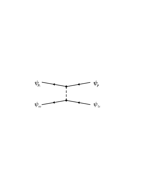
Figure 1: Feynman diagram for excitation of a K-shell electron into the bound $ns$ state by electron impact. Solid lines denote electrons in the external Coulomb field of the nucleus, while the dashed line denotes the electron-electron Coulomb interaction.

For non-relativistic energies $E_{p}$ within the asymptotic range $I(1-n^{-2})\ll E_{p}\ll m$, $E_{p_{1}}\sim E_{p}$ and the absolute value of the asymptotic momentum of the scattered electron is estimated as $p_{1}\sim p\gg\eta$. Accordingly, one needs to calculate only the Feynman diagram depicted in Fig. 1. The wave functions of both the incident and scattered high-energy electrons can be approximated by plane waves (Born approximation). The contribution of the exchange diagram turns out to be significantly suppressed and thus negligible. Using the expressions (7)–(9), the amplitude of the process can be represented as follows

$${\mathcal{A}} = 4\pi\alpha\,N_{1s}\frac{1}{q^{2}}\Bigl{(}-\frac{\partial}{\partial\lambda}\Bigr{)}\langle\psi_{{ns}}|V_{i\lambda}|\bm{q}\rangle_{\left|\vphantom{\bigl{(}}\,\lambda=\eta\right.}\,,$$ (17)

$$\langle\psi_{{ns}}|V_{i\lambda}|\bm{q}\rangle = N_{ns}\frac{\pi}{i\eta q}\biggl{\{}\frac{(\nu^{*}+\eta_{n})^{n}}{(\nu^{*}-\eta_{n})^{n}}-\frac{(\nu+\eta_{n})^{n}}{(\nu-\eta_{n})^{n}}\biggr{\}}\,,$$ (18)

where $N^{2}_{ns}=\eta_{n}^{3}/\pi$, $\nu=iq-\lambda$, and $\bm{q}=\bm{p}-\bm{p}_{1}$ is the momentum transfer. Although Eq. (18) is written in the complex form, it is a real function of the square of the momentum transfer $q^{2}$. In the limit $q^{2}\to 0$, Eq. (18) is in agreement with the expression (13). Taking the derivative with respect to $\lambda$ in Eq. (17) yields

$${\mathcal{A}} = 4\pi\alpha\,\eta^{-5}N_{1s}N_{ns}T_{n}(x)\,,$$ (19)

$$T_{n}(x) = \frac{2\pi}{ix^{3}}\biggl{\{}\frac{(ix-\tau_{-})^{n-1}}{(ix-\tau_{+})^{n+1}}-\frac{(ix+\tau_{-})^{n-1}}{(ix+\tau_{+})^{n+1}}\biggr{\}}\,,$$ (20)

where $x=q/\eta$ and $\tau_{\pm}=1\pm n^{-1}$. Note, that $T_{n}(x)$ is a real function depending actually on $x^{2}$.

The differential cross section for the $1s$-$ns$ excitation is related to the dimensionless function (20) via

$$d\sigma^{*}_{1s}(ns)=\frac{\sigma_{0}}{Z^{4}}\frac{4\,T_{n}^{2}(x)}{\pi^{2}n^{3}\varepsilon}\,dx^{2}\,,$$ (21)

where $\sigma_{0}=\pi a_{0}^{2}=87.974$ Mb. Here we have also introduced the dimensionless energy $\varepsilon=E_{p}/I$ of the incident electron. The energy-conservation law implies $\varepsilon=\varepsilon_{1}+1-n^{-2}$, where $\varepsilon_{1}=E_{p_{1}}/I$ denotes the dimensionless energy of the scattered electron. The asymptotic non-relativistic energy domain is characterized by $1-n^{-2}\ll\varepsilon\ll 2(\alpha Z)^{-2}$.

The leading high-energy contribution to the total cross section for the excitation process is given by

$$\sigma^{*}_{1s}(ns) = \frac{\sigma_{0}}{Z^{4}}\,Q_{n}(\varepsilon)\,,\quad(n\geqslant 2)\,,$$ (22)

$$Q_{n}(\varepsilon) = \frac{\varkappa_{n}}{n^{3}\varepsilon}\,,$$ (23)

$$\varkappa_{n} = \frac{8}{\pi^{2}}\int\limits_{0}^{\infty}dx\,x\,T_{n}^{2}(x)$$ (24)

$$= \frac{2^{6}}{(2n+1)!}\frac{d^{2n+1}}{dx^{2n+1}}\biggl{[}\frac{\ln x}{x^{5}}(x-i\tau_{-})^{2n-2}\biggr{]}_{\left|\vphantom{\bigl{(}}\,x=i\tau_{+}\right.}$$

$$-\frac{2^{7}}{n!}\frac{d^{n}}{dx^{n}}\biggl{[}\frac{\ln x}{x^{5}}\frac{(x^{2}+\tau^{2}_{-})^{n-1}}{(x+i\tau_{+})^{n+1}}\biggr{]}_{\left|\vphantom{\bigl{(}}\,x=i\tau_{+}\right.}\,.$$

In Eq. (24), we have chosen the regular branch of the logarithm, which assumes real values on the upper edge of the cut made along the positive semi-axis. The universal function $Q_{n}(\varepsilon)$ does not depend on the nuclear charge $Z$ and describes the excitation of states with the zeroth-order matrix element of the dipole transition 15 . The dimensionless quantity $\varkappa_{n}$, which is a function of the principal quantum number $n$, is presented for particular values of $n\leqslant 12$ in Table 4. In the limit $n\gg 1$, the coefficients $\varkappa_{n}$ tend to the asymptotic value $\varkappa_{n}\simeq 1.798$.

Let us make a few comments:

• Due to the crossing symmetry 12 , the Feynman graph depicted in Fig. 1 describes also the $1s$-$ns$ excitation by the high-energy positron impact. The exchange effect is absent at all. To get the amplitude for the process, one needs to make the following substitutions: $\bm{p}\rightleftharpoons-\bm{p}_{1}$, which do not alter expressions for the ionization cross section. Accordingly, Eqs. (22)–(24) are also valid for the case of the positron impact.

• Although we have considered the excitation process by the high-energy electron impact, Eqs. (22)–(24) are also valid for the case of fast projectiles with another mass $M$. The corresponding energy-conservation law still reads $E_{p}-I=E_{p_{1}}-I_{n}$, where $E_{p}=Mv^{2}/2$ and $I_{n}$ is given by Eq. (3). However, now it is convenient to calibrate the energies of the incident and scattered particle by the characteristic binding energy $\tilde{I}=M(\alpha Z)^{2}/2$, namely, $\varepsilon=E_{p}/\tilde{I}$ and $\varepsilon_{1}=E_{p_{1}}/\tilde{I}$. The dimensionless energy $\varepsilon=v^{2}/(\alpha Z)^{2}$ does not depend on the mass of the incident particle, while the energy-conservation law now implies $\varepsilon=\varepsilon_{1}+\mu(1-n^{-2})$, where $\mu=m/M$. The asymptotic energy range is characterized by $\mu(1-n^{-2})\ll\varepsilon\ll 2(\alpha Z)^{-2}$.

• To leading order of non-relativistic perturbation theory, the total cross section for impact excitation of helium-like ions from the ground state into the $1sns$ configuration is by a factor 2 as large as that $\sigma^{*}_{1s}(ns)$ for hydrogen-like ions, taking into account the number of target electrons.

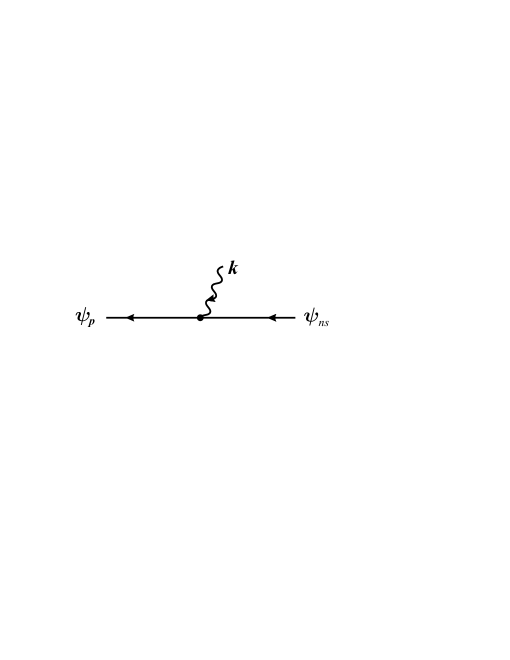
Figure 2: Feynman diagram for ionization of the bound $ns$ electron by photon impact.

5. The process of the single photoionization of a hydrogen-like ion in the $ns$ state is described by the diagram depicted in Fig. 2. The incident photon is characterized by the momentum $\bm{k}$, the energy $\omega=|\bm{k}|=k$, and the polarization vector $\bm{\mathrm{e}}$. The energy-conservation law reads $E_{p}=\omega-I_{n}$, where $E_{p}=\bm{p}^{2}/(2m)$ is the energy of the outgoing electron and $I_{n}$ is given by Eq. (3). Accordingly, the non-relativistic photoeffect can proceed at photon energies $I_{n}\leqslant\omega\ll m$. In the dipole approximation, the non-relativistic problem can be solved analytically 22 ; 23 ; 24 ; 25 ; 26 . Using the integral representation (8) for the Coulomb wave functions (7) yields the amplitude of the process under consideration in the closed form

$$\mathcal{A}_{ns} = 4\pi\eta^{-3}N_{\gamma}N_{ns}N_{p}(1-i\xi)(\bm{\mathrm{e}}\cdot\bm{p})\,\Phi_{n}(\xi)\,,$$ (25)

$$\Phi_{n}(\xi) = \frac{1}{(n-1)!}\frac{d^{n-1}}{dy^{n-1}}\biggl{[}\frac{y(y+n^{-1})^{n}}{(y^{2}+\xi^{-2})^{2}}\,e^{-2\xi\cot^{-1}(y\xi)}\biggr{]}_{\left|\vphantom{\bigl{(}}\,y=1/n\right.}\,,$$ (26)

$$N_{\gamma} = \frac{1}{m}\frac{\sqrt{4\pi\alpha}}{\sqrt{2\omega}}\,,\quad N^{2}_{ns}=\frac{\eta_{n}^{3}}{\pi}\,,\quad N^{2}_{p}=\frac{2\pi\xi}{1-e^{-2\pi\xi}}\,,$$ (27)

where $\xi=\eta/p$. Here we employ the Coulomb gauge, in which $(\bm{\mathrm{e}}\cdot\bm{k})=0$ and $(\bm{\mathrm{e}}^{*}\cdot\bm{\mathrm{e}})=1$. The dimensionless function (26) can be written as

$$\Phi_{n}(\xi)=\frac{e^{-2\xi\cot^{-1}(\xi/n)}}{(n^{2}+\xi^{2})^{n}}\,\xi^{4}f_{n}(\xi)\,,$$ (28)

where $f_{n}(\xi)$ for particular values of $1\leqslant n\leqslant 9$ are presented in Table 5. For large values of $n$, it is convenient to employ the recurrence relations between the matrix elements 22 ; 23 ; 24 ; 25 ; 26 .

The total cross section reads 23 ; 25

$$\sigma^{+}_{ns} = \frac{\sigma_{0}}{Z^{2}}F_{n}(\xi)\,,\quad n^{-2}\leqslant\varepsilon_{\gamma}\ll 2(\alpha Z)^{-2}\,,$$ (29)

$$F_{n}(\xi) = \frac{2^{7}\pi}{3n}\frac{(1+\xi^{2})\xi^{8}}{(1-e^{-2\pi\xi})}\frac{e^{-4\xi\cot^{-1}(\xi/n)}}{(n^{2}+\xi^{2})^{2n+1}}f^{2}_{n}(\xi)\,,$$ (30)

where $\sigma_{0}=\alpha\pi a_{0}^{2}=0.642$ Mb. Due to the energy-conservation law, the parameter $\xi=\eta/p$ corresponds to the dimensionless energy of the photon $\varepsilon_{\gamma}=\omega/I$ according to $\varepsilon_{\gamma}=\xi^{-2}+n^{-2}$. The universal function $F_{n}(\xi)$ does not depend on the nuclear charge number $Z$.

In the high-energy non-relativistic domain, which is characterized by $n^{-2}\ll\varepsilon_{\gamma}\ll 2(\alpha Z)^{-2}$, the amplitude (25) simplifies and appears as

$$\mathcal{A}_{ns}=N_{\gamma}N_{ns}\left(\bm{\mathrm{e}}\cdot\bm{p}\right)\frac{8\pi\eta}{q^{4}}=n^{-3/2}\mathcal{A}_{1s}\,.$$ (31)

Here $\bm{q}=\bm{p}-\bm{k}\simeq\bm{p}$, because the process proceeds with a large momentum transfer $q\gg\eta$. The total cross section reads 14

$$\sigma^{+}_{ns}=\frac{\sigma_{0}}{Z^{2}}\frac{2^{8}}{3n^{3}}\,\xi^{7}=\frac{\sigma^{+}_{1s}}{n^{3}}\,,$$ (32)

where $\xi\simeq\varepsilon_{\gamma}^{-1/2}$. The formula (32), which provides just the leading term in the expansion of Eq. (29) with respect to the parameter $\xi\ll 1$, can be obtained within the Born approximation. Since the function (30) involves also the parameter $\pi\xi$, which originates from the normalization factor of the Coulomb wave function of the continuous spectrum, the convergence of the $\xi$ expansion is sufficiently slow. Note also that, since the electron-nucleus binding for the excited $ns$ electron is weaker than that for the K-shell electron, the cross section $\sigma^{+}_{ns}$ is suppressed by the factor of $n^{-3}$ with respect to the cross section $\sigma^{+}_{1s}$. In the limiting case of a free electron, the cross section for single photoeffect tends to zero 12 .

6. Let us consider the single ionization of helium-like ions in the $1sns\,({}^{1,3}\!S)$ states by high-energy photon impact, which is not followed by excitation of the target. The principal quantum number $n$ is assumed to be $n\geqslant 2$. For the ground state, the problem has been studied in Ref. 27 . The process can proceed by two different channels. We shall start with ionization of the K-shell electron. Neglecting the electron-electron interaction, the amplitude of the process reads

$$\mathcal{A}^{(0)}_{\mathrm{I}}=\mathcal{A}_{1s}\,,$$ (33)

where $\mathcal{A}_{1s}$ is given by Eq. (31). The total cross section is just $\sigma_{1s}^{+}$ given by Eq. (32), that is, it keeps the same form for both the singlet and triplet states. The spin dependence appears, when one takes into account the electron-electron interaction.

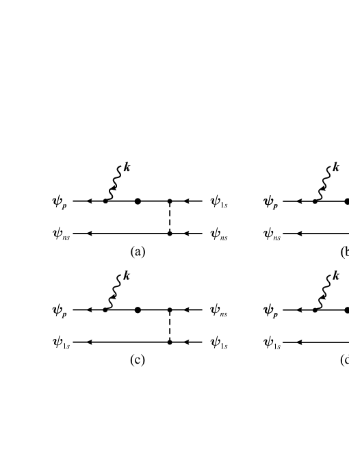
Figure 3: Feynman diagrams for single ionization of helium-like ion in the $1sns$ configurations following by the absorption of a high-energy photon. The lines with a heavy dot correspond to the reduced Coulomb Green’s functions. The diagrams (a) and (b) describe ionization of the K-shell electron, while diagrams (c) and (d) describe ionization of the $ns$ electron.

In first-order perturbation theory, the amplitude for the first ionization channel is $\mathcal{A}^{\vphantom{()}}_{\mathrm{I}}=\mathcal{A}^{(0)}_{\mathrm{I}}+\mathcal{A}^{(1)}_{\mathrm{I}}$. Within the high-energy asymptotic domain, the dominant contribution to the correlation correction $\mathcal{A}^{(1)}_{\mathrm{I}}$ arises only from the diagrams depicted in Figs. 3(a) and (b), while the other diagrams can be neglected. In explicit terms, one can write

$$\mathcal{A}^{(1)}_{\mathrm{I}} = \mathcal{A}^{(1)}_{\mathrm{a}}\pm\mathcal{A}^{(1)}_{\mathrm{b}}\,,$$ (34)

$$\mathcal{A}^{(1)}_{\mathrm{a}} = \alpha N_{\gamma}N_{1s}\left(\bm{\mathrm{e}}\cdot\bm{p}\right)\frac{\eta_{n}}{n^{2}}\frac{1}{(2\pi i)^{2}}\oint\limits^{(\eta_{n}^{+})}\!\prod\limits_{k=1}^{2}\biggl{[}dy_{k}\frac{(y_{k}+\eta_{n})^{n}}{(y_{k}-\eta_{n})^{n}}\biggr{]}$$ (35)

$$\times\Bigl{(}-\frac{\partial}{\partial\lambda}\Bigr{)}\frac{1}{\lambda^{2}}\langle\bm{q}|G_{\mathrm{R}}(E_{1s})\left(V_{i\eta}-V_{i(\lambda+\eta)}\right)|0\rangle_{\left|\vphantom{\bigl{(}}\,\lambda=y_{1}+y_{2}\right.}\,,$$

$$\mathcal{A}^{(1)}_{\mathrm{b}} = \alpha N_{\gamma}N_{1s}\left(\bm{\mathrm{e}}\cdot\bm{p}\right)\frac{\eta_{n}}{n^{2}}\frac{1}{(2\pi i)^{2}}\oint\limits^{(\eta_{n}^{+})}\!\prod\limits_{k=1}^{2}\biggl{[}dy_{k}\frac{(y_{k}+\eta_{n})^{n}}{(y_{k}-\eta_{n})^{n}}\biggr{]}$$ (36)

$$\times\Bigl{(}-\frac{\partial}{\partial\lambda}\Bigr{)}\frac{1}{\lambda^{2}}\langle\bm{q}|G_{\mathrm{R}}(E_{1s})\left(V_{iy_{2}}-V_{i(\lambda+y_{2})}\right)|0\rangle_{\left|\vphantom{\bigl{(}}\,\lambda=y_{1}+\eta\right.}\,.$$

Here again the momentum transfer is $\bm{q}=\bm{p}-\bm{k}\simeq\bm{p}$. In the derivation, we have used the Born approximation for the wave function of the ejected high-energy electron. In Eq. (34), the plus and minus signs correspond to the singlet and triplet states, respectively. For $q\gg\eta$, the matrix element involving the reduced Coulomb Green’s function $G_{\mathrm{R}}(E_{1s})$ was evaluated in the work 27 .

The correlation corrections for the amplitude can be cast into the following form

$$\mathcal{A}^{(1)}_{\mathrm{I}}=N_{\gamma}N_{1s}\dfrac{4\pi\eta}{Zq^{4}}\left(\bm{\mathrm{e}}\cdot\bm{p}\right)a^{\pm}_{1}\,.$$ (37)

The coefficients $a^{\pm}_{1}$, which correspond to the singlet and triplet states, are presented in Tables 6 and 7. In the limit $n\gg 1$, the product $n^{3}a^{+}_{1}$ tends to the asymptotic constant $-1.031$, while $n^{3}a^{-}_{1}$ approaches the value $0.087$. Employing Eqs. (33) and (37) yields the total amplitude for the single K-shell photoeffect

$$\mathcal{A}^{\vphantom{()}}_{\mathrm{I}}=\mathcal{A}^{(0)}_{\mathrm{I}}+\mathcal{A}^{(1)}_{\mathrm{I}}=\mathcal{A}^{(0)}_{\mathrm{I}}\Bigl{(}1+\dfrac{a^{\pm}_{1}}{2Z}\Bigr{)}\,,$$ (38)

which takes into account the electron correlations. The ionization cross section reads

$$\sigma^{+}_{\mathrm{I}}=\sigma_{1s}^{+}\left(1+a^{\pm}_{1}Z^{-1}\right)\,,$$ (39)

where $\sigma^{+}_{1s}$ is given by Eq. (32). As it is seen, account of the electron-electron interaction gives rise to the significant dependence of ionization cross sections on the spin multiplicity of atomic states. Indeed, the characteristic orbits of the $1s$ and $ns$ electrons are somewhat different. However, in the singlet state, both electrons are allowed to be at the same spatial point, while, in the triplet state, it is forbidden by the Pauli principle. Accordingly, in the $n\,{}^{1}\!S$ state, the account of the dominant correlation corrections attenuates the binding of the K-shell electron with the nucleus. As a result, the cross section decreases in comparison with the single-particle prediction (32). In the $n\,{}^{3}\!S$ state, the correlation corrections amplify the electron-nucleus binding for the K-shell electron, what makes the ionization cross section $\sigma^{+}_{\mathrm{I}}$ even a bit larger than $\sigma_{1s}^{+}$.

Another channel for the single photoeffect on helium-like ions in the $1sns\,({}^{1,3}\!S)$ states is ionization of the $ns$ electron. To leading order, the amplitude of the process reads

$$\mathcal{A}^{(0)}_{\mathrm{II}}=\mathcal{A}_{ns}\,,$$ (40)

where $\mathcal{A}_{ns}$ is given by Eq. (31). The total cross section coincides with the formula (32), being independent of the spin multiplicity of the wave functions.

To first order of the perturbation theory with respect to the electron-electron interaction, one needs to take into account the diagrams drawn in Figs. 3(c) and (d). The corresponding contributions can be represented as

$$\mathcal{A}^{(1)}_{\mathrm{c}} = 2\alpha\,\eta^{2}N_{\gamma}N_{ns}\left(\bm{\mathrm{e}}\cdot\bm{p}\right)\frac{1}{2\pi i}\oint\limits^{(\eta_{n}^{+})}\!dy\frac{(y+\eta_{n})^{n}}{(y-\eta_{n})^{n}}$$ (41)

$$\times\Bigl{(}-\frac{\partial}{\partial\lambda}\Bigr{)}\frac{1}{\lambda^{2}}\langle\bm{q}|G_{\mathrm{R}}(E_{ns})\left(V_{iy}-V_{i(\lambda+y)}\right)|0\rangle_{\left|\vphantom{\bigl{(}}\,\lambda=2\eta\right.}\,,$$

$$\mathcal{A}^{(1)}_{\mathrm{d}} = 2\alpha\,\eta^{2}N_{\gamma}N_{ns}\left(\bm{\mathrm{e}}\cdot\bm{p}\right)\frac{1}{2\pi i}\oint\limits^{(\eta_{n}^{+})}\!dy\frac{(y+\eta_{n})^{n}}{(y-\eta_{n})^{n}}$$ (42)

$$\times\Bigl{(}-\frac{\partial}{\partial\lambda}\Bigr{)}\frac{1}{\lambda^{2}}\langle\bm{q}|G_{\mathrm{R}}(E_{ns})\left(V_{i\eta}-V_{i(\lambda+\eta)}\right)|0\rangle_{\left|\vphantom{\bigl{(}}\,\lambda=y+\eta\right.}\,.$$

Here the matrix elements should be evaluated with the reduced Green’s function $G_{\mathrm{R}}(E_{ns})$ at the energy point $E_{ns}=-\eta^{2}_{n}/(2m)$, which is related to the usual non-relativistic Green’s function $G(E)$ via

$$G_{\mathrm{R}}(E_{ns})=\lim_{E\to E_{ns}}\biggl{\{}G(E)-\frac{|\psi_{ns}\rangle\langle\psi_{ns}|}{E-E_{ns}}\biggr{\}}\,.$$ (43)

For $q\gg\eta$, the Coulomb matrix element has the following integral representation 19

$$\langle\bm{q}|G(E)V_{i\lambda}|0\rangle\simeq 2^{5}\pi m\eta\frac{ip_{1}}{q^{4}}\int_{0}^{1}\frac{t^{-i\zeta}\,dt}{[\lambda-ip_{1}-(\lambda+ip_{1})t]^{2}}\,,$$ (44)

where $\zeta=\eta/p_{1}$ and $p_{1}=\sqrt{2mE}$ is the intermediate momentum. Performing the analytical continuation of Eq. (44) and canceling the pole terms according to the definition (43) yield

$$\langle\bm{q}|G_{\mathrm{R}}(E_{ns})V_{i\lambda}|0\rangle = 2^{5}\pi m\frac{\eta^{2}}{q^{4}}\biggl{\{}P_{n}(\lambda)+\biggr{.}$$ (45)

$$+(n+1)(\lambda-\eta_{n})^{n}\biggl{.}\int_{0}^{1}\frac{\ln t\,dt}{[\lambda(1-t)+\eta_{n}(1+t)]^{n+2}}\biggr{\}}\,.$$

The explicit expressions of the function $P_{n}(\lambda)$ for particular values of $n\leqslant 9$ are given in Table 8.

In the case of ionization of the $ns$ electron, it is convenient to introduce the correlation coefficients $b^{\pm}_{1}$ according to

$$\mathcal{A}^{(1)}_{\mathrm{II}}=\mathcal{A}^{(1)}_{\mathrm{c}}\pm\mathcal{A}^{(1)}_{\mathrm{d}}=N_{\gamma}N_{ns}\dfrac{4\pi\eta}{Zq^{4}}\left(\bm{\mathrm{e}}\cdot\bm{p}\right)b^{\pm}_{1}\,,$$ (46)

where plus and minus correspond to the singlet and triplet states, respectively. The coefficients $b^{\pm}_{1}$ are evaluated in Tables 9 and 10. In the asymptotic limit $n\gg 1$, $b^{+}_{1}$ tends to the constant $-1.47$, while $b^{-}_{1}$ approaches to the value $-2.44$. The total amplitude for ionization of the $ns$ electron is $\mathcal{A}^{\vphantom{()}}_{\mathrm{II}}=\mathcal{A}^{(0)}_{\mathrm{II}}+\mathcal{A}^{(1)}_{\mathrm{II}}$. The partial cross section for the second channel reads

$$\sigma^{+}_{\mathrm{II}}=\sigma_{ns}^{+}\left(1+b^{\pm}_{1}Z^{-1}\right)\,,$$ (47)

where $\sigma^{+}_{ns}$ is given by Eq. (32). As it is seen, account of the electron-electron interaction turns out to be crucial for describing the high-energy photoeffect on the $ns$ electron. Especially, it concerns the triplet states, where the screening corrections $b^{-}_{1}$ are very large. Due to the Pauli exclusion principle, the transfer of a large momentum from the nucleus to the $ns$ electron appears to be hardly probable. Accordingly, the ionization cross section strongly decreases in comparison with the single-particle approximation (32). Note that, for a neutral helium atom in the $n\,{}^{3}\!S$ state, Eq. (47) predicts negative values for $\sigma^{+}_{\mathrm{II}}$, if $n\geqslant 3$. In this case, one needs to take into account higher-order correlation corrections, which have not been considered in the present paper. For two-electron ions with $Z\geqslant 3$, the cross section (47) is always positive.

Taking into account both ionization channels, the total cross section for the single photoeffect on helium-like ions in the $1sns\,({}^{1,3}\!S)$ states reads

$$\sigma^{+} = \sigma^{+}_{\mathrm{I}}+\sigma^{+}_{\mathrm{II}}$$ (48)

$$= \sigma_{1s}^{+}\left(1+a^{\pm}_{1}Z^{-1}\right)+\sigma_{ns}^{+}\left(1+b^{\pm}_{1}Z^{-1}\right)\,.$$ (49)

In view of the relation (32), Eq. (49) can be also cast into the following form

$$\sigma^{+}=\sigma_{1s}^{+}\bigl{\{}1+n^{-3}+\left(a^{\pm}_{1}+n^{-3}b^{\pm}_{1}\right)Z^{-1}\bigl{\}}\,.$$ (50)

The coefficients $a^{\pm}_{1}$ and $b^{\pm}_{1}$ describe the dominant contribution to the correlation effect at high photon energies.

Although the expressions (49) and (50) have been derived within the Born approximation, Eq. (49) can be employed for a sufficiently wide energy domain, provided the single-particle cross sections are described by Eq. (29) 27 ; 28 . Indeed, the expression (29) keeps the same form to first order of the perturbation theory, taking into account the correlation corrections to the binding energy. However, for the high-energy domain characterized by $\varepsilon_{\gamma}^{-1}\ll\xi\ll 1$, the binding energy corrections are negligibly small with respect to the photon energy. Since the function (30) involves the correct dependence on the parameter $\xi$, Eq. (49) turns out to be also correct, neglecting terms of the order of about $(\xi/Z)^{2}=(m\alpha/p)^{2}$ (see also extensive discussions on this topic in Refs. 29 ; 30 ; 31 ; 32 ). In this paper, we have omitted some correlation corrections to the amplitude, which are of about $m\alpha/p$ (in particular, those, which arise due to the final-state interaction). However, the neglected terms are purely imaginary and do not contribute to the ionization cross section.

Concluding, we have investigated the processes of excitation and ionization of light multicharged ions by impact of high-energy particles, which proceed with participation of the $ns$ electrons. The dominant correlation corrections to the energy levels and photoionization cross sections are calculated analytically within the framework of non-relativistic perturbation theory. As major result, the universal scalings for the excitation and ionization cross sections are deduced.

Table 1: For the pure $ns^{2}\,({}^{1}\!S)$ states of helium-like ions, the dimensionless coefficients $\epsilon_{1}$ are tabulated according to Eq. (12).

$n$	$n^{2}\epsilon_{1}$		$n$	$n^{2}\epsilon_{1}$
	analytical	numerical		analytical	numerical
1	$5/4$	1.25	9	$2555635959/2147483648$	1.19006
2	$77/64$	1.20313	10	$40886039491/34359738368$	1.18994
3	$153/128$	1.19531	11	$81765970991/68719476736$	1.18985
4	$19541/16384$	1.19269	12	$10465450564505/8796093022208$	1.18978
5	$39043/32768$	1.19150	13	$20929978151879/17592186044416$	1.18973
6	$624353/524288$	1.19086	14	$334867944396713/281474976710656$	1.18969
7	$1248305/1048576$	1.19048	15	$669717016529889/562949953421312$	1.18966
8	$1277999141/1073741824$	1.19023	16	$5486195355159701189/4611686018427387904$	1.18963

Table 2: For the $1sns\,({}^{1}\!S)$ terms of helium-like ions, the dimensionless coefficients $\epsilon_{1}$ are tabulated according to Eqs. (14)–(16).

$n$	$n^{2}\epsilon_{1}$
	analytical	numerical
2	$1352/729$	1.8546
3	$31041/16384$	1.8946
4	$18741536/9765625$	1.9191
5	$87737225/45349632$	1.9347
6	$1319346413640/678223072849$	1.9453
7	$137428433691773/70368744177664$	1.9530
8	$294001828174792832/150094635296999121$	1.9588
9	$12270688433717907483/6250000000000000000$	1.9633
10	$160115079305309345784200/81402749386839761113321$	1.9669
11	$19575441723611998332463421/9937105900423855516680192$	1.9699
12	$180937160122853564881284932640/91733330193268616658399616009$	1.9724
13	$7619039446472988471652076553139/3858646740351497994569680683008$	1.9745
14	$8421485561700554490032347126878248/4261134649619646370410919189453125$	1.9763
15	$168262776200010701611816602447746396925/85070591730234615865843651857942052864$	1.9779

Table 3: For the $1sns\,({}^{3}\!S)$ terms of helium-like ions, the dimensionless coefficients $\epsilon_{1}$ are tabulated according to Eqs. (14)–(16).

$n$	$n^{2}\epsilon_{1}$
	analytical	numerical
2	$1096/729$	1.5034
3	$27639/16384$	1.6869
4	$17279264/9765625$	1.7694
5	$41200175/22674816$	1.8170
6	$1253464471368/678223072849$	1.8482
7	$131602743884003/70368744177664$	1.8702
8	$283169102583793792/150094635296999121$	1.8866
9	$1483842517395327999/781250000000000000$	1.8993
10	$155435328837703659864200/81402749386839761113321$	1.9095
11	$19056793993685438861087899/9937105900423855516680192$	1.9177
12	$176552744806540188413776122912/91733330193268616658399616009$	1.9246
13	$3724467497547548854690865614181/1929323370175748997284840341504$	1.9304
14	$8247164359458263840860888961901352/4261134649619646370410919189453125$	1.9354
15	$165016222122028120626234494334313260675/85070591730234615865843651857942052864$	1.9398

Table 4: For various values of the principal quantum number $n$, the dimensionless coefficients $\varkappa_{n}$ are calculated according to Eq. (24).

$n$	$\varkappa_{n}$
	analytical	numerical
2	$1048576/295245$	3.5515
3	$85293/35840$	2.3798
4	$806380109824/384521484375$	2.0971
5	$2815390625/1420541793$	1.9819
6	$2238980830283169792/1164315722505971035$	1.9230
7	$835179111639733/442209832796160$	1.8886
8	$156418330091764719082799104/83789232212292561749679885$	1.8668
9	$10197593930567041902351/5506157875061035156250$	1.8520
10	$580608990927250169145671680000000/315279866676074279955576140196657$	1.8416
11	$28550108411751156734369151319/15568186626467172764709027840$	1.8339
12	$9784817930963041730702096023760230416384/5352585600085746305433457063492098280775$	1.8280

Table 5: For various values of the principal quantum number $n$, the dimensionless functions $f_{n}(\xi)$ are tabulated according to Eqs. (26) and (28).

$n$		$f_{n}(\xi)$
1		$2/\left(1+{\xi}^{2}\right)$
2		$32$
3		$54\left(27+7{\xi}^{2}\right)$
4		$\left(512/3\right)\left(768+288{\xi}^{2}+23{\xi}^{4}\right)$
5		$\left(1250/3\right)\left(46875+20625{\xi}^{2}+2545{\xi}^{4}+91{\xi}^{6}\right)$
6		$\left(864/5\right)\left(25194240+12130560{\xi}^{2}+1827360{\xi}^{4}+105552{\xi}^{6}+2023{\xi}^{8}\right)$
7		$\left(4802/45\right)\left(12711386205+6485401125{\xi}^{2}+1097665170{\xi}^{4}+79704282{\xi}^{6}+2547265{\xi}^{8}+29233{\xi}^{10}\right)$
8		$\left(8192/315\right)\left(21646635171840+11499774935040{\xi}^{2}+2101597962240{\xi}^{4}+175037743104{\xi}^{6}+\right.$
		$\left.+7190401024{\xi}^{8}+140890496{\xi}^{10}+1044871{\xi}^{12}\right)$
9		$\left(4374/35\right)\left(2402063207770905+1314709492319055{\xi}^{2}+253715866938765{\xi}^{4}+23169940624971{\xi}^{6}+\right.$
		$\left.+1109810543211{\xi}^{8}+28441442925{\xi}^{10}+366767919{\xi}^{12}+1859129{\xi}^{14}\right)$

Table 6: For the $1sns\,({}^{1}\!S)$ terms of helium-like ions, the dimensionless coefficients $a^{+}_{1}$ are tabulated according to Eqs. (34)–(37).

$n$	$n^{3}a^{+}_{1}$
	analytical	numerical
2	$\left(8/2187\right)\left(-1679+3360\ln(3/2)\right)$	$-1.1582$
3	$\left(81/131072\right)\left(-24245+78184\ln(4/3)\right)$	$-1.0832$
4	$\left(192/48828125\right)\left(-7097629+30599840\ln(5/4)\right)$	$-1.0596$
5	$\left(125/3265173504\right)\left(-1171956731+6277663800\ln(6/5)\right)$	$-1.0491$
6	$\left(648/23737807549715\right)\left(-2411780852069+15397639065760\ln(7/6)\right)$	$-1.0435$
7	$\left(1029/5629499534213120\right)\left(-496846568524997+3678208705153360\ln(8/7)\right)$	$-1.0401$
8	$\left(512/47279810118554723115\right)\left(-11062929106398468157+93112579989061637760\ln(9/8)\right)$	$-1.0379$
9	$\left(729/3500000000000000000000\right)\left(-733561568265485829193+6915165610828616935920\ln(10/9)\right)$	$-1.0365$

Table 7: For the $1sns\,({}^{3}\!S)$ terms of helium-like ions, the dimensionless coefficients $a^{-}_{1}$ are tabulated according to Eqs. (34)–(37).

$n$	$n^{3}a^{-}_{1}$
	analytical	numerical
2	$\left(8/2187\right)\left(-1399+3552\ln(3/2)\right)$	$0.1507$
3	$\left(27/131072\right)\left(-67801+237576\ln(4/3)\right)$	$0.1123$
4	$\left(64/48828125\right)\left(-20509663+92256480\ln(5/4)\right)$	$0.1006$
5	$\left(125/1632586752\right)\left(-572430899+3146517000\ln(6/5)\right)$	$0.0955$
6	$\left(216/4747561509943\right)\left(-1424070240731+9251393817120\ln(7/6)\right)$	$0.0927$
7	$\left(2401/5629499534213120\right)\left(-210463375781159+1577733920822640\ln(8/7)\right)$	$0.0911$
8	$\left(512/6754258588364960445\right)\left(-1566435008617827011+13309413901475690880\ln(9/8)\right)$	$0.0901$
9	$\left(729/437500000000000000000\right)\left(-91055968618569041179+864741335682205139760\ln(10/9)\right)$	$0.0893$

Table 8: For various values of the principal quantum number $n$, the functions $P_{n}(\lambda)$ are tabulated according to Eq. (45).

$n$		$P_{n}(\lambda)$
1		$\dfrac{2\eta}{\left(\eta+\lambda\right)^{3}}-\dfrac{5}{2\left(\eta+\lambda\right)^{2}}$ $\frac{\vphantom{\Bigl{(}}}{\vphantom{\Bigl{(}}}$
2		$\dfrac{1}{8\eta_{2}^{2}}-\dfrac{3\lambda^{2}}{\left(\lambda+{\eta_{2}}\right)^{4}}-\dfrac{\lambda}{2\left(\lambda+{\eta_{2}}\right)^{3}}+\dfrac{5}{4\left(\lambda+{\eta_{2}}\right)^{2}}$ $\frac{\vphantom{\bigl{(}}}{\vphantom{\Bigl{(}}}$
3		$\dfrac{\lambda}{24\eta_{3}^{3}}-\dfrac{16\lambda^{3}}{3\left(\lambda+{\eta_{3}}\right)^{5}}+\dfrac{14\lambda}{3\left(\lambda+{\eta_{3}}\right)^{3}}-\dfrac{5}{3\left(\lambda+{\eta_{3}}\right)^{2}}$ $\frac{\vphantom{\bigl{(}}}{\vphantom{\Bigl{(}}}$
4		$\dfrac{\lambda^{2}}{64\eta_{4}^{4}}-\dfrac{\lambda}{48\eta_{4}^{3}}+\dfrac{5}{192\eta_{4}^{2}}-\dfrac{10\lambda^{4}}{\left(\lambda+\eta_{4}\right)^{6}}+\dfrac{7\lambda^{3}}{3\left(\lambda+\eta_{4}\right)^{5}}+\dfrac{13\lambda^{2}}{\left(\lambda+\eta_{4}\right)^{4}}-\dfrac{39\lambda}{4\left(\lambda+\eta_{4}\right)^{3}}+\dfrac{47}{24\left(\lambda+\eta_{4}\right)^{2}}$ $\frac{\vphantom{\bigl{(}}}{\vphantom{\Bigl{(}}}$
5		$\dfrac{\lambda^{3}}{160\eta_{5}^{5}}-\dfrac{\lambda^{2}}{64\eta_{5}^{4}}+\dfrac{\lambda}{60\eta_{5}^{3}}+\dfrac{1}{192\eta_{5}^{2}}-\dfrac{96\lambda^{5}}{5\left(\lambda+\eta_{5}\right)^{7}}+\dfrac{148\lambda^{4}}{15\left(\lambda+\eta_{5}\right)^{6}}+\dfrac{472\lambda^{3}}{15\left(\lambda+\eta_{5}\right)^{5}}-\dfrac{38\lambda^{2}}{\left(\lambda+\eta_{5}\right)^{4}}+\dfrac{232\lambda}{15\left(\lambda+\eta_{5}\right)^{3}}-$ $\frac{\vphantom{\bigl{(}}}{\vphantom{\bigl{(}}}$
		$-\dfrac{131}{60\left(\lambda+\eta_{5}\right)^{2}}$ $\frac{\vphantom{\bigl{(}}}{\vphantom{\Bigl{(}}}$
6		$\dfrac{\lambda^{4}}{384\eta_{6}^{6}}-\dfrac{3\lambda^{3}}{320\eta_{6}^{5}}+\dfrac{13\lambda^{2}}{960\eta_{6}^{4}}-\dfrac{7\lambda}{960\eta_{6}^{3}}+\dfrac{17}{1920\eta_{6}^{2}}-\dfrac{112\lambda^{6}}{3\left(\lambda+\eta_{6}\right)^{8}}+\dfrac{464\lambda^{5}}{15\left(\lambda+{\eta_{6}}\right)^{7}}+\dfrac{208\lambda^{4}}{3\left(\lambda+{\eta_{6}}\right)^{6}}-\dfrac{368\lambda^{3}}{3\left(\lambda+{\eta_{6}}\right)^{5}}+$ $\frac{\vphantom{\bigl{(}}}{\vphantom{\bigl{(}}}$
		$+\dfrac{229\lambda^{2}}{3\left(\lambda+{\eta_{6}}\right)^{4}}-\dfrac{65\lambda}{3\left(\lambda+{\eta_{6}}\right)^{3}}+\dfrac{71}{30\left(\lambda+{\eta_{6}}\right)^{2}}$ $\frac{\vphantom{\bigl{(}}}{\vphantom{\Bigl{(}}}$
7		$\dfrac{\lambda^{5}}{896\eta_{7}^{7}}-\dfrac{\lambda^{4}}{192\eta_{7}^{6}}+\dfrac{67\lambda^{3}}{6720\eta_{7}^{5}}-\dfrac{3\lambda^{2}}{320\eta_{7}^{4}}+\dfrac{71\lambda}{13440\eta_{7}^{3}}+\dfrac{1}{240\eta_{7}^{2}}-\dfrac{512\lambda^{7}}{7\left(\lambda+{\eta_{7}}\right)^{9}}+\dfrac{2992\lambda^{6}}{35\left(\lambda+{\eta_{7}}\right)^{8}}+\dfrac{4944\lambda^{5}}{35\left(\lambda+{\eta_{7}}\right)^{7}}-$ $\frac{\vphantom{\bigl{(}}}{\vphantom{\bigl{(}}}$
		$-\dfrac{2476\lambda^{4}}{7\left(\lambda+{\eta_{7}}\right)^{6}}+\dfrac{2104\lambda^{3}}{7\left(\lambda+{\eta_{7}}\right)^{5}}-\dfrac{129\lambda^{2}}{\left(\lambda+\eta_{7}\right)^{4}}+\dfrac{989\lambda}{35\left(\lambda+\eta_{7}\right)^{3}}-\dfrac{353}{140\left(\lambda+{\eta_{7}}\right)^{2}}$ $\frac{\vphantom{\bigl{(}}}{\vphantom{\Bigl{(}}}$
8		$\dfrac{\lambda^{6}}{2048\eta_{8}^{8}}-\dfrac{5{\lambda}^{5}}{1792\eta_{8}^{7}}+\dfrac{289\lambda^{4}}{43008\eta_{8}^{6}}-\dfrac{29\lambda^{3}}{3360\eta_{8}^{5}}+\dfrac{457\lambda^{2}}{71680\eta_{8}^{4}}-\dfrac{53\lambda}{26880\eta_{8}^{3}}+\dfrac{919}{215040\eta_{8}^{2}}-\dfrac{144\lambda^{8}}{\left(\lambda+\eta_{8}\right)^{10}}+\dfrac{7704\lambda^{7}}{35\left(\lambda+{\eta_{8}}\right)^{9}}+$ $\frac{\vphantom{\bigl{(}}}{\vphantom{\bigl{(}}}$
		$+\dfrac{1328\lambda^{6}}{5\left(\lambda+\eta_{8}\right)^{8}}-\dfrac{4722\lambda^{5}}{5\left(\lambda+\eta_{8}\right)^{7}}+\dfrac{1032\lambda^{4}}{\left(\lambda+\eta_{8}\right)^{6}}-\dfrac{1193\lambda^{3}}{2\left(\lambda+\eta_{8}\right)^{5}}+\dfrac{984\lambda^{2}}{5\left(\lambda+\eta_{8}\right)^{4}}-\dfrac{1407\lambda}{40\left(\lambda+\eta_{8}\right)^{3}}+\dfrac{1487}{560\left(\lambda+\eta_{8}\right)^{2}}$ $\frac{\vphantom{\bigl{(}}}{\vphantom{\Bigl{(}}}$
9		$\dfrac{\lambda^{7}}{4608\eta_{9}^{9}}-\dfrac{3\lambda^{6}}{2048\eta_{9}^{8}}+\dfrac{275\lambda^{5}}{64512\eta_{9}^{7}}-\dfrac{99\lambda^{4}}{14336\eta_{9}^{6}}+\dfrac{17\lambda^{3}}{2520\eta_{9}^{5}}-\dfrac{279\lambda^{2}}{71680\eta_{9}^{4}}+\dfrac{523\lambda}{322560\eta_{9}^{3}}+\dfrac{207}{71680\eta_{9}^{2}}-\dfrac{2560\lambda^{9}}{9\left(\lambda+\eta_{9}\right)^{11}}+$ $\frac{\vphantom{\bigl{(}}}{\vphantom{\bigl{(}}}$
		$+\dfrac{56864\lambda^{8}}{105\left(\lambda+\eta_{9}\right)^{10}}+\dfrac{141952\lambda^{7}}{315\left(\lambda+\eta_{9}\right)^{9}}-\dfrac{107168\lambda^{6}}{45\left(\lambda+\eta_{9}\right)^{8}}+\dfrac{48416\lambda^{5}}{15\left(\lambda+\eta_{9}\right)^{7}}-\dfrac{21236\lambda^{4}}{9\left(\lambda+\eta_{9}\right)^{6}}+\dfrac{46952\lambda^{3}}{45\left(\lambda+\eta_{9}\right)^{5}}-$ $\frac{\vphantom{\bigl{(}}}{\vphantom{\bigl{(}}}$
		$-\dfrac{1402\lambda^{2}}{5\left(\lambda+\eta_{9}\right)^{4}}+\dfrac{13348\lambda}{315\left(\lambda+\eta_{9}\right)^{3}}-\dfrac{6989}{2520\left(\lambda+\eta_{9}\right)^{2}}$ $\frac{\vphantom{\bigl{(}}}{\vphantom{\Bigl{(}}}$

Table 9: For the $1sns\,({}^{1}\!S)$ terms of helium-like ions, the dimensionless coefficients $b^{+}_{1}$ are tabulated according to Eqs. (41), (42), and (46).

$n$	$b^{+}_{1}$
	analytical	numerical
2	$\left(4/2187\right)\left(-772+159\ln 3\right)$	$-1.0925$
3	$\left(3/131072\right)\left(-73875+13816\ln 4\right)$	$-1.2525$
4	$\left(72/48828125\right)\left(-1248684+219365\ln 5\right)$	$-1.3207$
5	$\left(5/3265173504\right)\left(-1268946065+213266808\ln 6\right)$	$-1.3580$
6	$\left(12/23737807549715\right)\left(-3996048740304+649245311015\ln 7\right)$	$-1.3814$
7	$\left(7/5629499534213120\right)\left(-1674319803898931+264724373084400\ln 8\right)$	$-1.3974$
8	$\left(16/47279810118554723115\right)\left(-6304966995252184568+974522181024852075\ln 9\right)$	$-1.4090$
9	$\left(9/3500000000000000000000\right)\left(-847067488481686729599+128414477117971809520\ln 10\right)$	$-1.4178$

Table 10: For the $1sns\,({}^{3}\!S)$ terms of helium-like ions, the dimensionless coefficients $b^{-}_{1}$ are tabulated according to Eqs. (41), (42), and (46).

$n$	$b^{-}_{1}$
	analytical	numerical
2	$\left(4/2187\right)\left(-1604+543\ln 3\right)$	$-1.8426$
3	$\left(3/131072\right)\left(-146181+41032\ln 4\right)$	$-2.0439$
4	$\left(8/48828125\right)\left(-22143244+5629965\ln 5\right)$	$-2.1434$
5	$\left(5/1632586752\right)\left(-1254848345+298760904\ln 6\right)$	$-2.2037$
6	$\left(12/4747561509943\right)\left(-1589311619664+360435860155\ln 7\right)$	$-2.2444$
7	$\left(21/5629499534213120\right)\left(-1116056979027599+243593185902000\ln 8\right)$	$-2.2737$
8	$\left(16/6754258588364960445\right)\left(-1810645396585286728+382953780229600125\ln 9\right)$	$-2.2959$
9	$\left(9/437500000000000000000\right)\left(-213879211569028496997+44048190258616320560\ln 10\right)$	$-2.3133$

References

• (1) B.H. Bransden, M.R.C. McDowell, Phys. Rep. 46 (1978) 249.
• (2) R.J.W. Henry, Phys. Rep. 68 (1981) 1.
• (3) Y. Itikawa, Phys. Rep. 143 (1986) 69.
• (4) H. Knudsen, J.F. Reading, Phys. Rep. 212 (1992) 107.
• (5) Y. Itikawa, Atomic Data Nucl. Data Tables 63 (1996) 315.
• (6) V.I. Fisher, Y.V. Ralchenko, V.A. Bernshtam, A. Goldgirsh, Y. Maron, L.A. Vainshtein, I. Bray, H. Golten, Phys. Rev. A 55 (1997) 329.
• (7) J. Eichler, Th. Stöhlker, Phys. Rep. 439 (2007) 1.
• (8) A.I. Mikhailov, I.A. Mikhailov, A.V. Nefiodov, G. Plunien, G. Soff, Pis’ma Zh. Eksp. Teor. Fiz. 78 (2003) 141, JETP Lett. 78 (2003) 110.
• (9) A.I. Mikhailov, I.A. Mikhailov, A.V. Nefiodov, G. Plunien, Phys. Lett. A 355 (2006) 363.
• (10) A.I. Mikhailov, A.V. Nefiodov, G. Plunien, Phys. Rev. Lett. 97 (2006) 233003.
• (11) A.V. Nefiodov, G. Plunien, Phys. Lett. A 363 (2007) 115.
• (12) V.B. Berestetskii, E.M. Lifshits, L.P. Pitaevskii, Quantum Electrodynamics (2nd ed.), Pergamon Press, London, 1982.
• (13) The use of the same notations for the electron mass and projection of the orbital angular momentum is not confusing, because the latter is related with the angular dependence of wave functions only.
• (14) H.A. Bethe, E.E. Salpeter, Quantum Mechanics of One- and Two-Electron Atoms, Plenum, New York, 1977.
• (15) L.D. Landau, E.M. Lifshits, Quantum Mechanics: Non-relativistic Theory, third ed., Pergamon Press, London, 1977.
• (16) C. Sinha, N. Roy, N.C. Sil, J. Phys. B 11 (1978) 1807.
• (17) C. Sinha, N.C. Sil, J. Phys. B 12 (1979) 1711.
• (18) A.K. Das, N.C. Sil, J. Phys. B 17 (1984) 3987.
• (19) M.Ya. Amusia, A.I. Mikhailov, Zh. Eksp. Teor. Fiz. 111 (1997) 862, JETP 84 (1997) 474.
• (20) V.M. Galitskii, B.M. Karnakov, V.I. Kogan, Problems in quantum mechanics, Nauka, Moscow, 1992.
• (21) A.V. Nefiodov, G. Plunien, Phys. Lett. A (2007), doi:10.1016/j.physleta.2007.06.053.
• (22) W. Gordon, Ann. Phys. (Leipzig) 2 (1929) 1031.
• (23) M. Stobbe, Ann. Phys. (Leipzig) 7 (1930) 661.
• (24) L.C. Biedenharn, J.L. McHale, R.M. Thaler, Phys. Rev. 100 (1955) 376.
• (25) A. Burgess, Mem. Roy. Astron. Soc. 69 (1965) 1.
• (26) G. Soff, J. Rafelski, Z. Phys. D 14 (1989) 187.
• (27) A.I. Mikhailov, A.V. Nefiodov, G. Plunien, Phys. Lett. A 358 (2006) 211.
• (28) A.I. Mikhailov, A.V. Nefiodov, G. Plunien, Phys. Lett. A 368 (2007) 391.
• (29) T. Surić, E.G. Drukarev, R.H. Pratt, Zh. Eksp. Teor. Fiz. 124 (2003) 243, JETP 97 (2003) 217.
• (30) T. Surić, E.G. Drukarev, R.H. Pratt, Phys. Rev. A 67 (2003) 022709; ibid. 67 (2003) 059902, Erratum.
• (31) T. Surić, R.H. Pratt, J. Phys. B 37 (2004) L93.
• (32) T. Surić, Rad. Phys. Chem. 70 (2004) 253.
Refer to caption