A Macroscopic Description of Coherent Geo-Magnetic Radiation from Cosmic Ray Air Showers

Abstract

We have developed a macroscopic description of coherent electro-magnetic radiation from air showers initiated by ultra-high energy cosmic rays due to the presence of the geo-magnetic field. This description offers a simple and direct insight in the relation between the properties of the air shower and the time-structure of the radio pulse.

I Introduction

In recent years the interest in the use of radio detection for cosmic ray air showers is increasing with the promising results obtained from recent LOPES Fal05 ; Ape06 and CODALEMA Ard06 experiments. These experiments have in turn triggered plans to install an extensive array of radio detectors at the Pierre Auger Observatory Ber07 . There is thus a growing interest the link between the properties of the air shower and the time structure of the emitted pulse. Already in the earliest works on radio emission from air showers Jel65 ; Por65 ; Kah66 ; All71 , the importance of coherent emission was stressed. Two mechanisms, Cherenkov radiation and geo-magnetic radiation were proposed as possibilities. In more recent work Fal03 ; Sup03 ; Hue03 , the picture of coherent synchrotron radiation from secondary shower electrons and positrons gyrating in the Earth’s magnetic field was proposed. Extensive results on geo-synchrotron emission, based on realistic Monte-Carlo simulations of the shower development, are given in Hue05 ; Hue07 .

The primary motivation of this work is to improve on the understanding of the relation between the measured pulse shape using radio receivers and the properties of the air shower induced by a cosmic ray. Therefore, we performed macroscopic calculations which allow, under simplifying conditions, to obtain a simple analytic expression for the pulse shape. This analytic expression shows a clear relation between the pulse shape and the shower profile.

The picture we use is very similar to that used in Ref. Kah66 which we refine by using a more realistic shower profile and where we calculate the time-dependence of the pulse. The magnetic field of the Earth induces, by pulling with the Lorentz force the electrons and positrons in opposite directions, a net electric current in the electron-positron plasma. This plasma moves with almost the velocity of light towards the Earth at the front end of the cosmic-ray air shower. In our approach the collective aspect is emphasized by treating this induced current as macroscopic. This differs from the approach of Refs. Hue05 ; Hue07 where the motion of individual particles is stressed (microscopic approach). In both the macroscopic and the microscopic approach the emission of the electromagnetic pulse is caused by moving charges in the Earth’s magnetic field. Therefore these two pictures should be regarded as presenting a complementary view of the same physical phenomenon. There are however differences in the predicted pulse shapes and we hope that by presenting this complementary picture the understanding of radio emission from extensive air showers can be improved.

In the introduction of Section II the basic outline of our approach is presented and the various aspects are detailed in the different subsections. Starting from a very basic picture we present our results in Section III. Subsequently the effects on the pulse shape are investigated of finite lateral extend, finite pancake thickness, and a realistic energy distribution of the electrons and positrons in the air shower.

II The Formalism

When an UHE cosmic-ray particle enters the upper layers of the atmosphere, a cascade of high-energy particles – called a cosmic-ray air shower – develops. Due to the high velocities, most of the particles are concentrated in the relatively thin shower front, which, for obvious reasons, is called the ’pancake’. The pancake, which for the present discussion is assumed to be charge neutral, contains extremely large numbers of electrons and positrons. Near the core of the shower this pancake has a typical thickness of a few meters and is moving to the surface of the Earth with (almost) the velocity of light through the magnetic field of the Earth. The Lorentz force on the charged particles induces an acceleration of the particles in the $\hat{x}$ direction, which is perpendicular to the magnetic field and the shower axis. However, due to the frequent collision with the air-molecules, where the relatively small transverse velocity is randomized, this acceleration, when averaged over all electrons, rather translates into a drift velocity and thus an electric current in the $\hat{x}$ direction. This picture is similar to what happens to electrons in a copper wire. When a voltage is applied over the wire, the electrons undergo a constant acceleration due to the electric force which is however compensated by collisions with the copper atoms, resulting in a constant drift velocity and thus a constant electric current. At the surface of the Earth, electromagnetic radiation can be detected, which is due to this relatively constant electric current moving with high velocity towards the Earth. The shape of the electromagnetic pulse is principally determined by the (relatively slow) variation in time of the magnitude of the current, combined with time retardation effects.

To emphasize the basic principles, we confine ourselves to a rather simple geometry where the cosmic shower moves straight towards the Earth’s surface (the $-\hat{z}$ direction, see Fig. 1) with velocity $\vec{v}_{s}=-\beta_{s}c\hat{z}$ where $\beta_{s}\approx 1$. The position of the shower front above the Earth’s surface is given by $z=-\beta_{s}ct$, where the front of the shower reaches Earth at time $t=0$. The Earth’s magnetic field (with magnitude $B_{E}$) is parallel to the surface (in the $\hat{y}$ direction), $\vec{B}=B_{E}\hat{y}$. The strength of the induced electric current depends on the distance $h$ from the front of the shower and on the time $t$ in the shower development. The direction of the current is in the $\hat{x}$ direction. All quantities are measured in the rest system of the observer who is at rest at the surface of the Earth.

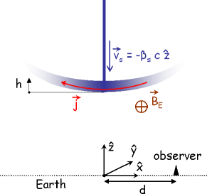
Figure 1: [color online] The basic geometry as used in this paper. The pancake is shown as the shaded area, moving with velocity $\vec{v}_{s}$. The observer is at a distance $d$ from the point of impact. The curvature of the pancake has not been included in the present calculations.

In the calculation of the current density we will initially assume a finite extent in the horizontal directions (x and y). However, soon we will integrate over these variables, knowing that the charged-particle density is strongly peaked near the center of the shower. To emphasize the importance of the distance $h$ behind the shower front, we will write the electron/positron density as

$$\rho_{e}(x,y,z,t)=\int\tilde{\rho}_{e}(x,y,z,t,h)dh\;,$$ (1)

where we assume a simple factorized form,

$$\tilde{\rho}_{e}(x,y,z,t,h) = N_{e}\delta(z+\beta_{s}ct+h)$$ (2)

$$\times f_{t}(t)\rho_{\mbox{\tiny NKG}}(x,y)\rho_{p}(h)\;.$$

The total number of charged particles at the time of maximum shower development is denoted as $N_{e}$. The velocity of the shower front is given by $\vec{v}_{s}=-\beta_{s}c\hat{z}$. The lateral distribution function is normalized according to $\int\rho_{\mbox{\tiny NKG}}(x,y)\,dx\,dy=1$, the pancake distribution obeys a similar normalization, $\int\rho_{p}(h)\,dh=1$, and the maximum of the temporal (or longitudinal) distribution $f_{t}(t)$ is normalized to unity. A detailed discussion of the parameterizations for these shower functions is given in the appendix. In Section A.4 also the effects of an energy spread of the electrons and positrons are considered.

To emphasize the collective aspects of the model the calculation of the drift velocity of the electrons and positrons is treated as a separate topic. The magnitude of the induced current is calculated as the number of electrons (and positrons) multiplied by an average drift velocity. In the following stage this is combined with the shower profile to calculate the emitted electromagnetic pulse.

II.1 Magnitude of the Current

For the present estimate it is assumed that there are equal numbers of positive and negative charges moving towards the Earth with a large velocity. Due to the Earth’s magnetic field a net electrical current in the $\hat{x}$-direction is induced with magnitude

$$j(x,y,z,t)=\int\langle v_{d}q\rangle\,e\,\tilde{\rho}_{e}(x,y,z,t,h)dh\;,$$ (3)

where $\tilde{\rho_{e}}$ is the density of electrons and positrons, Eq. (2). To take into account that the electrons and positrons ($q=-1,+1$ respectively) drift in opposite directions under the influence of the magnetic field, the average sidewards drift velocity is weighted with the charge, denoted as $\langle v_{d}q\rangle$.

The radius of curvature of orbits of the electrons with an energy $\epsilon_{e}=\gamma mc^{2}$ in the Earth’s magnetic field is $R_{B}=\beta\gamma mc/(eB_{E})$. A realistic magnitude of the magnetic field ($B_{E}=0.3\times 10^{-4}$ T) yields a curvature radius $R_{B}=\beta\gamma\times 50$ m. The angular deflection is thus $\theta=L/R_{B}$ where $L$ is the mean free path, i.e. the length over which the electrons scatter over a large angle due to multiple soft scattering or a hard scattering. The transverse component of the velocity is $v_{t}=c\theta=cLeB_{E}/(\beta\gamma mc)$, assuming that $\sin{\theta}\ll 1$ or a transverse velocity much smaller than the longitudinal component. The drift velocity, being the average over the complete trajectory, is half this value remark1 ,

$$v_{d}=c\theta/2={cLeB_{E}\over 2\beta\gamma mc}.$$ (4)

The problem is thus now reduced to the calculation of the mean path length $L$.

At high energies, $\epsilon_{e}>10$ MeV, the electron cross section is dominated by hard collisions and the mean path length is given by $L_{R}=X_{0}/\rho_{air}$, where the electronic radiation length is $X_{0}=36.7$ g cm^-2 and the density of air is $\rho_{air}=10^{-3}$ g cm^-3 at sea level. The density is of course lower at higher altitudes.

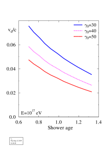
Figure 2: [color online] The drift velocity as function of shower age for different values of $\gamma_{0}$ in the multiple Compton scattering contribution, Eq. (6). The range in shower age corresponds to an elevation from 10 km up to sea level.

For smaller energies the above considerations do not apply since Coulomb scattering becomes the dominant scattering mechanism with a mean free path between successive collisions of 1 g cm^-2 (which can be determined directly from the corresponding cross sections). Since Coulomb scattering is strongly forward peaked, several collisions are necessary to randomize the momentum. As argued in Ref. Gai90 the scattering angle due to multiple Coulomb scattering after traversing a distance $d$, is $\delta\langle\theta^{2}\rangle=d(\gamma_{0}/\gamma)^{2}\rho_{air}/X_{0}$ with $\gamma_{0}=40$. When $\delta\langle\theta^{2}\rangle\approx 1$, the original direction is lost, giving an effective path length $L_{C}=(\gamma/\gamma_{0})^{2}X_{0}/\rho_{air}$. Over the whole energy range, the average path length $L$ may be written as $1/L=1/L_{C}+1/L_{R}$ or

$$L={\gamma^{2}\over\gamma^{2}+\gamma_{0}^{2}}{X_{0}\over\rho_{air}}\;.$$ (5)

The drift velocity, obtained from Eqs.(4,5), now reads

$$v_{d}={c\over 2\,\beta}{\gamma\over\gamma^{2}+\gamma_{0}^{2}}{eB_{E}\over mc}{X_{0}\over\rho_{air}}\;,$$ (6)

keeping the energy dependence of the average path length. The average drift velocity is finally obtained by averaging over the energy distribution of electrons in a cosmic-ray air shower, using a parametrization given in Ref. Ner06 (see also Eq. (31)). Since this velocity is small, our assumption $\sin{\theta}\ll 1$ is indeed valid.

The drift velocity depends rather strongly on the assumptions made in the estimate of multiple Coulomb scattering, as can be seen from Fig. 2 by choosing different values for $\gamma_{0}$. The height dependence in $\langle v_{d}q\rangle$ is due to the change in $\rho_{air}$ and due to the fact that the energy distribution of particles in the shower pancake depends on shower age Ner06 . In the present calculations we used a constant drift velocity, $\langle v_{d}q\rangle=0.04$ c, equal to the value at the shower maximum for $\gamma_{0}=40$.

In Section III the results obtained using the average current density is compared to the one obtained by explicitly integrating the electric field generated by the particles of different energies. The difference between the two appears to be mainly a normalization of the field strength, while the pulse shape is hardly affected.

II.2 The vector Potential

Given a current density, $j^{\mu}$, the vector potential can be obtained using the Liénard-Wiechert fields,

$$A^{\mu}(x)={1\over 4\pi\varepsilon_{0}}\int\left.{j^{\mu}\over R(1-\vec{\beta}\cdot\hat{n})}\right|_{\mbox{ret}}\,dh\;,$$ (7)

for a source with an infinitesimally small lateral extension. We use the common notation where $\hat{n}$ is a unit vector pointing from the source to the observer and $R$ is the distance, both evaluated at retarded time. Assuming that all particles move with the velocity of the shower front, the denominator in Eq. (7) can be rewritten to give

$${\cal D} = R(1-\vec{\beta_{s}}\cdot\hat{n})|_{\mbox{ret}}={c\over n}(t-t_{r})-n\beta_{s}(h-c\beta_{s}t_{r})$$ (8)

$$= \sqrt{(-c\beta_{s}t+h)^{2}+(1-\beta_{s}^{2}n^{2})d^{2}}\;,$$

using Eq. (34) for the retarded time. Eq. (8) is written for a general medium with an index of refraction $n$ however all our calculations are done in the limit $n=1$. The distance between the observer and the point of impact of the core of the air shower is denoted by $d$, see Fig. 1.

Since the current density has only an $\hat{x}$-component, the vector potential will share this property,

$$A^{x}(t,d)=J\int dh{\rho_{p}(h)f_{t}(t_{r})\over{\cal D}}\;,$$ (9)

where $\cal D$ is defined in Eq. (8) and where the current density is assumed to be parameterized according to Eq. (3) with $J=\langle v_{d}q\rangle N_{e}e/4\pi\varepsilon_{0}c$. We use SI units where ${e\over 4\pi\varepsilon_{0}}=1.44\times 10^{-9}$ [Vm] to get $E$ in [V/m]. The expression for the vector potential shown in Eq. (9) is the central equation in our derivation.

II.2.1 Charge Conservation, Static Dipole

At the point above the Earth’s surface where the shower front passes, the charges are being pulled apart by the Lorentz force. The air shower can thus be regarded as a ‘zipper’, pulling apart positive and negative charges at the point where it passes, leaving behind an electric dipole distributed along the path of the air shower. Since we have argued that the electric current, which is associated with the separating of the charges, is driving the electromagnetic pulse, we should also investigate the effects of the created dipole. This dipole radiates because it is not constant in time. To estimate its magnitude and the induced radiation field, we will assume that the pancake thickness is infinitely small. Please note that this dipole differs from the dipole mentioned in Kah66 which is co-moving with the air shower.

For definiteness, we temporarily assume that the charges are homogeneously distributed over a distance $w$ in the $\hat{x}$ direction (this assumption will be relaxed at the end). For a shower front at an height $z$ this corresponds to a line-charge density $N_{e}f_{t}(-z/\beta_{s}c)/w$. Since the charges move sideways with a velocity $\langle v_{d}q\rangle$, a charge $\Delta q=\pm\Delta t\,\langle v_{d}q\rangle\,N_{e}f_{t}(-z/\beta_{s}c)/w$ accumulates at $x=\pm w/2$ after a time $\Delta t$. We will assume that this charge is at rest in the Earth’s reference system and remains fixed at all later times while in reality it will slowly diffuse. Since the shower front progresses with a velocity $\beta_{s}c$, vertical line-charge densities $\pm\rho_{0}(z)$ are created a distance $w$ apart with

$$\rho_{0}(z)={\langle v_{d}q\rangle\,N_{e}f_{t}(-z/\beta_{s}c)\over c\beta_{s}w}\;.$$ (10)

These charge densities at height $z$ give a contribution to the zeroth component of the vector potential of magnitude

$$\delta A^{0} = {1\over 4\pi\varepsilon_{0}}\rho_{0}(z)\Big{(}{1\over R^{+}}-{1\over R^{-}}\Big{)}$$ (11)

$$= {1\over 4\pi\varepsilon_{0}}{w\,\rho_{0}(z)\,x\over R^{3}}=J{x\over c\beta_{s}R^{3}}f_{t}({-z\over\beta_{s}c})\;,$$

where we have introduced the distance $R=\sqrt{z^{2}+d^{2}}$ with $d^{2}=x^{2}+y^{2}$ and $R^{\pm}=\sqrt{z^{2}+(x\mp w/2)^{2}+y^{2}}$. From Eq. (11) it is clear that the assumption of a homogeneous line-charge density can be relaxed at this point. The scalar potential is obtained by integrating upward from the shower front over $z$,

$$A^{0}(t,d) = J{x\over c\beta_{s}}\int_{z_{0}}^{\infty}dz{f_{t}(-z/\beta_{s}c)\over R^{3}}\;,$$ (12)

where at time $t_{r}$ the shower front has reached a height of $z_{0}=-\beta_{s}ct_{r}$. The charges are now taken into account for the full development of the shower. It should, however, be noted that gauge condition, $\partial_{\mu}A^{\mu}$, is not fulfilled since in the present simple model we have assumed that the charges forming the dipole moment are at rest in the Earth’s system, while before they were moving with a vertical velocity $\beta_{s}c$. This sudden acceleration introduces an additional bremsstrahlung contribution which is beyond the scope of the present work.

II.2.2 Moving Dipole

In the pancake, by virtue of the induced current, there will also be an induced electric dipole moving towards the Earth with the shower velocity. We will argue here that this dipole will not generate a contribution to the pulse in the limit used in this paper, $n\beta_{s}=1$.

Due to the action of the Lorentz force the electrons and positrons will be displaced an average distance $s$. The contribution to the vector potential can now be written as

$$\Delta^{m}A^{0}(t,d) \propto \Big{(}{1\over{\cal D}^{+}}-{1\over{\cal D}^{-}}\Big{)}=s{\partial\over\partial x}{1\over{\cal D}}$$ (13)

$$= s{x(1-\beta_{s}^{2}n^{2})\over{\cal D}^{3}}$$

using the same notation as introduced in Eq. (11) and calculate the derivative from Eq. (8). This contribution vanishes in the limit $n\beta_{s}=1$ and will be ignored in the following.

II.3 The Electric Field

The electric and magnetic fields can be derived from the vector potential in the usual way,

$$\vec{E}(t,d)=-\partial_{0}\vec{A}(t,d)\;,$$ (14)

where we have ignored the zeroth component of the vector potential (see the discussion at the end of this Section).

Since the vector potential Eq. (9) has only a component in the $\hat{x}$ direction this will give rise to an electric field in the same direction. The emitted radiation is thus linearly polarized in the $\hat{x}$ direction, i.e. perpendicular to the shower axis and the magnetic field.

The upper limit of the integral over $h$ in Eq. (14) extends up to infinity and we obtain

$$E_{x}(t,d)=-J{d\over dt}\int_{0}^{\infty}dh{\rho_{p}(h)f_{t}(t_{r})\over{\cal D}}$$ (15)

$$= -J\int_{0}^{\infty}\!\!dh\,\rho_{p}(h){d\over dt}{f_{t}(t_{r})\over{\cal D}}$$

$$= -J\int_{0}^{\infty}\!\!dh\,{f_{t}(t_{r})\over{\cal D}}c\beta_{s}{d\,\rho_{p}(h)\over dh}$$

$$- J\int_{0}^{\infty}\!\!dh\,\rho_{p}(h)\Big{(}{d\over dt}+c\beta_{s}{d\over dh}\Big{)}{f_{t}(t_{r})\over{\cal D}}$$

$$- \left.c\beta_{s}\,\rho_{p}(h){f_{t}(t_{r})\over{\cal D}}\right|_{h=0}\;.$$

The second term can be rewritten as

$$\Big{(}{d\over dt}+c\beta_{s}{d\over dh}\Big{)}{f_{t}(t_{r})\over{\cal D}}$$ (16)

$$= {1\over{\cal D}}\Big{(}{dt_{r}\over dt}+c\beta_{s}{dt_{r}\over dh}\Big{)}{df_{t}(t_{r})\over dt_{r}}={df_{t}(t_{r})\over dt_{r}}{1\over{\cal D}}\;.$$

Using $\rho_{p}(h)=0$ for $h=0$, the expression for the electric field simplifies to

$$E_{x}(t,d) = -J\int_{0}^{\infty}dh\,{f_{t}(t_{r})\over{\cal D}}\beta{d\,\rho_{p}(h)\over dh}$$ (17)

$$-J\int_{0}^{\infty}dh\,{\rho_{p}(h)\over{\cal D}}{df_{t}(t_{r})\over dt_{r}}\;,$$

where one should be careful in evaluating the integral because of the $1/\sqrt{c\beta_{s}t-h}$ pole in ${1\over{\cal D}}$. To investigate the effect of this pole, associated with Cherenkov emission, we have explicitly studied the case $\beta_{s}n>1$ for which the pole in ${1\over{\cal D}}$ lies inside the integration region. Only for unrealistically large values for the index of refraction Cherenkov radiation is emitted by the electric current density. For realistic values of $n$ this effect is too small to distinguish. Since we see that our predicted pulse shapes for realistic values of $n$ and $n=1$ are identical we have limited ourselves to the latter.

II.3.1 Limiting Case

To obtain a simple estimate for the emitted radiation one may take the limit $\beta_{s}=1$ and $n=1$ and ignore the thickness of the pancake, giving

$${\cal D}=c\beta_{s}t+{\cal O}(1-\beta_{s}^{2})\approx ct$$ (18)

and, for positive values of $t$,

$$ct_{r}={ct\over 1+\beta_{s}}-{d^{2}\over 2c\beta_{s}t}+{\cal O}(1-\beta_{s}^{2})\approx-{d^{2}\over 2ct}\;,$$ (19)

which is large and negative since $d^{2}\gg c^{2}t^{2}$. Interesting to note here is that the earlier part of the signal ($t$ small and positive) contains the information of the earlier parts (at higher altitude) of the air-shower development ($t_{r}$ large and negative). The electric field can now be calculated, using $\int dh\,\rho_{p}(h)h\approx 0$, $\int dh\,\rho_{p}(h)=1$

$$E_{x}(t,d) = -J{n^{2}\sqrt{d^{2}+c^{2}\beta_{s}^{2}t_{r}^{2}}\over c{\cal D}^{2}}{df_{t}(t_{r})\over dt_{r}}$$ (20)

$$+ Jf_{t}(t_{r}){c\beta_{s}^{2}t\over{\cal D}^{3}}\;.$$

In the limit $\beta_{s}=1$ and $n=1$ Eq. (20) can be simplified further to,

$$E_{x}(t,d)\approx J{c^{2}t_{r}^{2}4\over d^{4}}\left[t_{r}{df_{t}(t_{r})\over dt_{r}}+f_{t}(t_{r})\right]\;.$$ (21)

The limit $t\to 0$ should be taken with care since this limit corresponds to large (and negative) retarded times, see Eq. (19), where the air shower may not even have started. As a result Eq. (21) produces a finite electric field at all times. For small distances to the shower core, $d\approx ct$, the approximations made in deriving the expression for the retarded time, Eq. (19), are no longer valid and Eq. (21) thus not applicable.

From Eq. (21) it can be seen that the time structure of the pulse is, independent of the distance, given by a rather simple function of the longitudinal shower profile. If at distance $d$ the peak of the pulse occurs at time $t_{0}$, at twice the distance, the signal peak occurs at a time $4\times t_{0}$ and the signal is four times as broad. From Eq. (21) it can be seen that the peak value of the field, occurring at the same retarded time, has decreased by a factor $2^{4}$. It should be noted that the emitted radiation does not contain a relativistic Lorentz $\gamma$ factor and therefore does not depend on the exact velocity of the shower front, as long as it is close to $c$. The dependence on the energy distribution of the particles in the shower pancake is only indirectly through the dependence of the drift velocity.

Eq. (21) shows that there is a direct relation between shower profile and the pulse structure. The calculations presented in Section III indicate that for a realistic case this feature is smeared out due to the effects of the finite extend of the pancake and the lateral distribution.

II.3.2 Dipole Field

To obtain an estimate of the effect of omitting the zeroth component of the vector potential from our discussion the contribution due to the electric dipole, Eq. (12), to the electric field is calculated as

$$-{dA^{0}\over dx} = \Delta E_{x}=J\left.{nf_{t}(-z/\beta_{s}c)x^{2}\over{\cal D}R^{3}}\right|_{z=z_{0}}$$ (22)

$$+J\int_{z_{0}}^{\infty}dz\,{f_{t}(-z/\beta_{s}c)\over\beta_{s}}{z^{2}+y^{2}-2x^{2}\over R^{5}}\;,$$

using ${d\,z_{0}\over dx}={n\beta_{s}x\over{\cal D}}$. Following a similar approach we obtain for the other components

$$\Delta E_{y} = J\left.{nf_{t}(-z/\beta_{s}c)x\,y\over{\cal D}R^{3}}\right|_{z=z_{0}}$$ (23)

$$+J\int_{z_{0}}^{\infty}\!dz\,{f_{t}(-z/\beta_{s}c)\over\beta_{s}}{-3x\,y\over R^{5}}\;,$$

$$\Delta E_{z} = J\left.{nf_{t}(-z/\beta_{s}c)x\,z\over{\cal D}R^{3}}\right|_{z=z_{0}}$$ (24)

$$-J\int_{z_{0}}^{\infty}\!dz\,{f_{t}(-z/\beta_{s}c)\over\beta_{s}}{3x\,z\over R^{5}}\;.$$

It is important to note that in Eqs. (22-24) the distance $R$ appears in the denominator in stead of ${\cal D}$ as in Eq. (17). The reason for this is that the electric dipole is at rest in the frame of the observer. Since $R\gg{\cal D}$ for the cases of practical interest, the contribution of Eq. (22) is much smaller than that of Eq. (17) and thus can safely be ignored.

II.4 Azimuthal Distribution of Radiation Pattern

As remarked before, the emitted electric field due to the induced electric current, Eq. (17), is linearly polarized in the $\hat{x}$-direction. Its magnitude depends only on the distance to the shower core and, for a shower with a cylindrical symmetry, has a perfect azimuthal symmetry around the point of impact of the shower. This symmetry is broken by the fact that, due to the drift velocity which is induced by the magnetic field, the distribution of charged particles in the shower is somewhat more stretched in the $\hat{x}$-direction than in the $\hat{y}$-direction. In addition, the field of the induced dipole, Eq. (22) and Eq. (23), does not have an azimuthal symmetry. The symmetry breaking induced by these two effects is however small and will not be considered further.

III Results

 

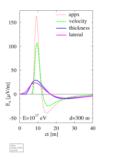
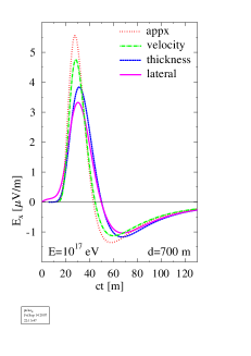
Figure 3: [color online] Effects of refinements of the shower structure on pulse shape at $300$ m and $700$ m from the shower core for a $10^{17}$ eV shower. The line labeled ’appx’ corresponds to the limiting case of Eq. (21) while the other curves include the effects of the finite pancake thickness, the lateral extent of the shower and the energy distribution of electrons in the shower as discussed in the text.

In Fig. 3 the calculated pulses as a function of time are shown at distances of 300 m and 700 m from the shower core for different levels of sophistication in the air-shower parametrization. The dotted curve, labeled ‘appx’, is the result of the most simple calculation using Eq. (21) where the longitudinal profile is given by Eq. (28). It has been verified that this result is indistinguishable from that obtained using the full expression, Eq. (17), in the limit of vanishing pancake thickness. In order to investigate the accurateness of this simple result as compared to a more realistic calculation we relax some of the approximations to see their effects.

In arriving at Eq. (17), the sideways drift velocity of the electrons and positrons has been averaged over their energy distribution. In doing so, the dependence of the denominator of Eq. (7) on electron energy has been ignored. To test the effect of this approximation we have instead used the full expression, see Eq. (32), resulting in the dash-dotted curves labeled ‘velocity’ in Fig. 3, still in the limit of vanishing pancake thickness. It shows that the effects of a spread in the energies of the electrons and positrons in the pancake affects mainly the magnitude of the pulse and hardly its time structure. At small distances the decrease of the peak height due to this effect is stronger than at large distances.

Including a finite thickness of the pancake, using Eq. (17) with Eq. (29), results in the curves labeled ‘thickness’ in Fig. 3. This has a very important effect on the pulse shape at 300 m, which can easily be understood since a finie pancake thickness, $L=c\Delta t$, introduces a ‘smearing’ effect for the pulse over a time $\Delta t$. Since for larger distances the pulse width is already sizable (it increases roughly with the second power of the distance as follows from Eqs. (19) and (21)) the smearing has only a minor effect at 700 m.

Taking in to account the effects of the lateral spread of the particles in the shower, Eq. (30), in addition to the pancake thickness, results in drawn curve labeled ‘lateral’ in Fig. 3. The width of the pulse increases even further although the effect is relatively small.

The effect of the static dipole field is shown in Fig. 4, where it is compared with the pulse including the effects of a finite pancake thickness, for two distances from the core. It should be noted that the dipole pulse has been multiplied by a factor $10^{3}$ in order to be able to show it on the same scale. This clearly shows the assertion made earlier that the dipole response can be safely ignored. Apart from the small magnitude, also the associated long wave length will make it undetectable in realistic experiments.

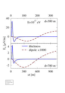
Figure 4: [color online] Comparing the pulse due to the dipole field with that of the current at two distances from the shower core.

For a realistic shower one should expect a strong correlation between charged particle velocity and the distance behind the shower front (slower particles trailing further behind). For this reason we have chosen not to mix the effects of the velocity distribution and finite pancake thickness in the present work which is based on using simple parameterized showers. Results for a full Monte-Carlo simulation will be presented in a future work, which will also take into account the effects of an angular spread of the particles in the pancake.

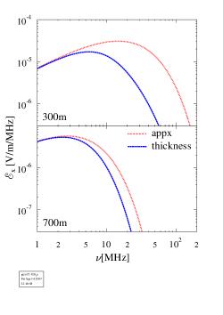
Figure 5: [color online] Frequency response of the pulse at two distances from the shower core. In the calculations labeled ’appx’ and ’thickness’ the thickness of the pancake is zero (Eq. (21)) and 10 m respectively.

The effect of a finite pancake thickness can also be seen in the frequency response of the pulse as shown in Fig. 5. The frequency response is normalized such that $\int|E(t)|^{2}dt=2\int|{\cal E}(\nu)|^{2}d\nu$. At shorter distances $d$, the effect of finite thickness is to suppress the higher frequency components since the signal is only coherent for wave lengths larger than the typical size of the emitting system. The signal, in the limit where the thickness is ignored, does depend strongly on the distance from the shower core since the projected longitudinal extend enters, which equals to zero when viewing the shower head-on. Including a finite thickness reduces the dependence of the pulse shape on the distance from the core.

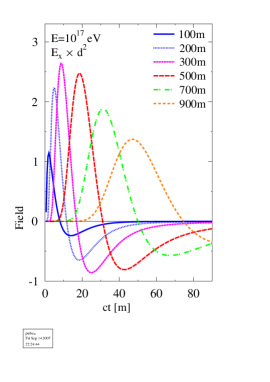
Figure 6: [color online] Electric field strength (multiplied by $d^{2}$) at different distances from the shower core as function of time.

In Fig. 6 the electric field is plotted as function of time for an observer at various distances $d$ from the shower core. The primary energy is $10^{17}$ eV and the calculation includes the effects of the pancake thickness only. The shower core hits the Earth’s surface at $t=0$. At large distances the pulse decreases in magnitude even faster than $d^{2}$, as predicted by Eq. (21). At small distances important deviations from the simple parametrization are observed. This is to a minor extent due to the fact that the approximations made to arrive at Eq. (21) are no longer valid, and mostly due to the effects of taking into account the finite thickness of the pancake which strongly influences the pulse shape at distances $d<500$ m. Including lateral extent of the shower will not greatly alter the picture.

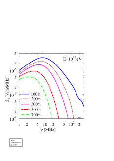
Figure 7: [color online] Fourier components of the electric field strength at different distances from the shower core for a $10^{17}$ eV shower.

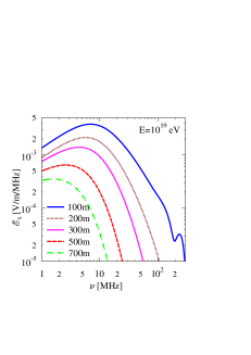
Figure 8: [color online] Same as Fig. 7 for a $10^{19}$ eV shower.

The frequency decomposition of the pulses shown in Fig. 6 are shown in Fig. 7 and those for an energy of $10^{19}$ eV in Fig. 8. At higher energies the shower maximum is closer to the surface of the Earth making for a broader pulse. This is reflected in the frequency spectrum by a peaking of the response at lower frequencies. At the same time the number of charged particles in the shower is roughly proportional to the energy of the primary particle. This in turn implies that the electric field is two orders of magnitude larger for a $10^{19}$ eV induced shower than for $10^{17}$ eV.

The present results can be compared with those given in Refs. Hue05 ; Hue07 . The basic features and magnitudes of the frequency responses are very similar. A difference is seen in the time structure of the peak. The pulse form obtained in this work has a distinct bi-polar structure, as has been discussed before, while that of Refs. Hue05 ; Hue07 has a simple unipolar structure. The bi-polar structure of the pulse can also be understood from the fact that the vector potential is positive definite and vanishes for both small and large times. The electric field is the time derivative of this vector potential and crosses zero at the time when the vector potential reaches a maximum. For the first part of the pulse the two terms in Eq. (21) add constructively resulting it the large leading positive part. Since the vanishing vector potential at $t=0$ and $t=\infty$ does not depend on details of the shower profile (radial distribution or velocity distribution) the predicted bi-polar shape, with a vanishing time-integral or zero-frequency component, can be regarded as a robust prediction. This prediction also follows from the work of ref. Kah66 . The main difference between this work and ref. Kah66 lies in the fact that we have considered a more realistic shower profile and have presented a calculation directly in the time domain. The latter allowed us to show explicitly the relation between shower profile and pulse shape.

IV Summary

In this work a relatively simple macroscopic picture is presented for the emission of coherent electromagnetic radiation from an extensive air shower initiated by a high-energy cosmic ray. In this picture the radiation is emitted through the electromagnetic current which is induced by the Earth’s magnetic field in the plasma at the front end of the shower. Under some simplifying assumptions a simple algebraic equation can be derived, Eq. (21), which clearly shows which are the important aspects of the air shower that determine the electromagnetic pulse.

It is shown that the time structure of the pulse directly reflects the longitudinal development of the number of electrons (and positrons) in the shower. The radio pulse, therefore, gives very similar information on the air shower as is obtained from air-fluorescence detection. Since the zero cross-over point of the pulse is related to the maximum in the shower profile this implies that the peak in the pulse is related to the shower development well before the maximum.

In this first paper we have restricted ourselves to a very simple geometry. In a future publication emission from showers for a more general geometry will be investigated.

Appendix A Air-Shower Parametrization

The front of the shower moves with a velocity $\beta_{s}c$ in the $-z$ direction, towards the Earth were the point $z=0$ is taken at the Earth’s surface. At time $t=0$ the shower reaches the surface of the Earth. The shower thus exists at negative times only.

The number of charged particles in the shower is parameterized as function of time ($t$), distance from the shower front ($h$), and lateral distance ($r=\sqrt{x^{2}+y^{2}}$) where we consider here vertical showers only. For simplicity we assume that the different dependencies simply factorize

$$\tilde{\rho}_{e}(x,y,z,t,h)=N_{e}f_{t}(t)\rho_{\mbox{\tiny NKG}}(x,y)\rho_{p}(h)\delta(z+\beta_{s}ct+h)\;.$$

The distributions $\rho_{p}(h)$ and $\rho_{\mbox{\tiny NKG}}(r)$ NKG are normalized such that their integrals equal to unity. The total number of charged particles at a specific time is thus given by $N_{e}f_{t}(t)$. This simple parametrization of the shower is sufficient to gain insight into the basic structure of the emitted electromagnetic pulse.

A.1 Longitudinal Profile

Following Ref. Hue03 , the longitudinal shower development can be parameterized using a shower age,

$$s(X)={3X/X_{0}\over X/X_{0}+2X_{\mbox{\tiny mx}}/X_{0}}\;,$$ (25)

where $X_{0}$=36.7 g/cm² is the electronic radiation length in air. The primary energy is denoted by $E_{p}$ and $X$ the penetration depth in units of [g cm^-2]. The parameter $X_{\mbox{\tiny mx}}$ is chosen such as to reproduce the positions of the shower maxima as have been determined from shower simulations Kna03 ,

$$X_{\mbox{\tiny mx}}=\Big{(}840+70\log_{10}(E_{p}/10^{20}\;eV)\Big{)}\;\mbox{g\,cm${}^{-2}$}\;.$$ (26)

In the present calculations we model the atmosphere as

$$X(z)=X(0)e^{-Cz}$$ (27)

with $X(0)=1000$ g cm^-2 and where $C$ is chosen such that $X(4\mbox{km})=630$ g cm^-2. Following Ref. Hue03 the time dependence of the number of charged particles is parameterized as

$$N_{e}f_{t}(t)=N_{e}e^{(X-X_{\mbox{\tiny mx}}-1.5X\ln{s})/X_{0}}\;,$$ (28)

using Eq. (27) with $z=-\beta_{s}t$. The maximum number of charged particles is chosen as $N_{e}=6\times(E_{p}/10^{10}\;eV)$ to agree with the number given in Kna03 for a $10^{19}$ eV shower.

A.2 Pancake Thickness

In Ref. Agn97 the measured arrival time distribution at a given radial distance is fitted with a $\Gamma$-probability distribution function ($\Gamma$-pdf). Converted into a thickness of the shower front this can be written as Hue03

$$\rho_{p}(h)=h^{\beta}e^{-2h/L}\times(4/L^{2})\;,$$ (29)

where the parameters $\beta$=1 and $L$ depend on shower age. At the shower maximum a reasonable choice for the parameters is given by $\beta$=1 and $L=10$ m. In the present calculation we keep these fixed for the full development of the shower. The effects the curvature of the pancake has been ignored.

A.3 Lateral Distribution

The lateral particle density can be described with the NKG (Nishimura-Kamata-Greisen) NKG parametrization, which at the shower maximum ($s=1$) reads

$$\rho_{\mbox{\tiny NKG}}(x,y)={1\over r^{2}_{M}}{2.5\over 2\pi}\Big{(}{r\over r_{M}}\Big{)}^{-1}\Big{(}{1+{r\over r_{M}}}\Big{)}^{-3.5}\;,$$ (30)

normalized such that $2\pi\,\int_{0}^{\infty}r\,dr\rho_{\mbox{\tiny NKG}}(x,y)=1$. Here $r_{M}$ is the Molière radius at the atmospheric height of the maximum derived from the atmospheric density as Dov03 $r_{M}(h)={9.6g\,cm^{-2}\over\rho_{atm}(h)}$. The atmospheric density at a height of 4 km corresponds to $\rho_{atm}=0.82$ mg cm^-3, which in turn yields $r_{M}\approx 117$ m.

A.4 Energy Distribution

In addition to the spatial distribution of the electrons in the shower, we have also taken their spread in energy into account. All the time we assume that the shower front is moving towards the Earth with velocity $\beta_{s}\approx 1$. The distribution of electron energies ${\epsilon_{e}}$ in the shower is taken to be $\rho_{E}(\epsilon_{e})$, where the parametrization is taken from Ref. Ner06 ,

$${d\rho_{E}(\epsilon_{e})\over d\log{\epsilon_{e}}}={\cal N}{\epsilon_{e}\over(\epsilon_{e}+\alpha)(\epsilon_{e}+\beta)^{s}}\;.$$ (31)

This parametrization is based on a detailed comparison with the results of Monte-Carlo calculations. The parameters are taken as Ner06 $\alpha=6.42522-1.53183s$ and $\beta=168.168-42.1368s$ in units of MeV where we have implemented this parametrization for shower age $s=1$. The normalization constant ${\cal N}$ is chosen to normalize the integral to unity.

The energy distribution of the electrons and positrons can be included in the present calculation at two levels of sophistication. The simplest is to use it only in the calculation of the average drift velocity as discussed in Section II.1. In a somewhat more sophisticated approach the contribution to the vector potential, Eq. (9), is averaged resulting in

$$A^{x}=\int_{0}^{\beta_{s}}{\rho_{E}(\epsilon_{e})v_{d}(\beta)\over R+\beta\beta_{s}t_{r}c}N_{e}f_{t}(t_{r})d\log{\epsilon_{e}}\;,$$ (32)

where $t_{r}$ is negative and the shower is at height $z_{0}=-\beta_{s}t_{r}c$. The denominator can be rewritten as $R+\beta\beta_{s}t_{r}c={\cal D}+z_{0}(\beta_{s}-\beta)$. The shower front moves with velocity $\beta_{s}c$ while the charged particles move with a smaller velocity and thus must be trailing behind the front at a certain distance. The latter effect has not been included here. From the vector potential the electric field can be calculated in the usual way.

Appendix B Retarded Time

At the retarded time $t_{r}$ the front of the shower is at a height $z=-c\beta_{s}t_{r}$. The travel time for a signal emitted at a distance $h$ behind the shower front at $z$ to reach the observer (at Earth at distance $d$ from the point of impact on Earth) is

$$t-t_{r}=\Delta t=n\sqrt{d^{2}+(z+h)^{2}}/c\;,$$ (33)

where $n$ is the index of refraction. The expression for the retarded time can thus be written as

$$c\,t_{r}={c\,t-n^{2}\beta_{s}h-n\sqrt{(-c\beta_{s}t+h)^{2}+(1-\beta_{s}^{2}n^{2})d^{2}}\over 1-\beta_{s}^{2}n^{2}}\;$$ (34)

where in our convention the retarded time is negative for a shower above the Earth and $t$ is assumed to be positive (the pulse, at a certain distance $d$, arrives only after the shower has hit the ground).

References

- (1) H. Falcke, et al., Nature 435, 313 (2005).
- (2) W. D. Apel, et al., Astropart. Physics 26, 332 (2006).
- (3) D. Ardouin, et al., Astropart. Physics 26, 341 (2006).
- (4) A.M. van den Berg for the Pierre Auger Collaboration, ICRC 2007 abstract
- (5) H. R. Allan, Prog. in Element. part. and Cos. Ray Phys. 10, 171 (1971).
- (6) F.D. Kahn and I.Lerche, Proc. Royal Soc. London A289, 206 (1966).
- (7) N.A. Porter, C.D. Long, B. McBreen, D.J.B Murnaghan and T.C. Weekes, Phys. Lett. 19, 415 (1965).
- (8) J. V. Jelley et al., Nature 205, 327 (1965).
- (9) T. Huege, H. Falcke, Astronomy & Astrophysics 412, 19 (2003).
- (10) H. Falcke and P. Gorham, Astropart. Phys. 19, 477 (2003).
- (11) D.A. Suprun, P.W. Gorham, J.L. Rosner, Astropart. Phys. 20, 157 (2003).
- (12) T. Huege, H. Falcke, Astronomy & Astrophysics 430, 779 (2005); T. Huege, H. Falcke, Astropart. Phys. 24, 116 (2005).
- (13) T. Huege, R. Ulrich, and R. Engel, Astropart. Phys. 27, 392 (2007)
- (14) T.K. Gaisser, ‘Cosmic Rays and Particle Physics’, Cambridge University Press, 1990.
- (15) F. Nerling et al., Astropart. Phys. 24, 421 (2006).
- (16) K. Greisen, Prog. Cosmic Ray Phys. Vol. 3 (1956) 1; K. Kamata, J. Nishimura, Prog. Theoret. Phys. Suppl. Vol. 6 (1958) 93.
- (17) J. Knapp et al., Astropart. Phys. 19, 77 (2003); astro-ph/0206414.
- (18) G. Agnetta, et al., Astropart. Phys. 6, 301 (1997).
- (19) M.T. Dova, et al., Astropart. Phys. 18, 351 (2003).
- (20) In ref. Kah66 the current is calculated using the transverse velocity at the end of the trajectory instead of the average which makes the current density a factor 2 larger in ref. Kah66 .