Spin squeezing and maximal-squeezing time

Abstract

Spin squeezing of a nonlinear interaction model with Josephson-like coupling is studied to obtain time scale of maximal squeezing. Based upon two exactly solvable cases for two and three particles, we find that the maximal-squeezing time depends on the level spacing between the ground state and its next neighbor eigenstate.

I INTRODUCTION

The phenomenon of spin squeezing in collective spin system have attracted much attention for decades not only because of fundamental physical interests Kitagawa ; Wineland ; Wineland1 ; Wineland2 ; Wineland3 ; Kuzmich ; Hald ; Geremia ; Rojo , but also for its possible application in atomic clocks for reducing quantum noise Wineland ; Wineland1 ; Wineland2 ; Wineland3 and quantum information Sorensen ; You ; Wang ; Lewenstein ; Yi . The occurrence of spin squeezing is due to quantum correlations among individual spins, which requires at least two spins and nonlinear interaction between them. Kitagawa and Uea have studied the spin squeezing generated by the so-called one-axis twisting (OAT) model with Hamiltonian: $\hat{H}_{\text{OAT}}=2\kappa\hat{J}_{z}^{2}$ Kitagawa . Possible realization of the OAT-type squeezing in a two-component Bose-Einstein Condensate (TBEC) Sorensen ; Molmer , and atomic ensemble system in a dispersive regime Takeuchi have been investigated recently. Sørensen et al. also proposed that the spin squeezing can be used as a measure of many-particle quantum entanglement Sorensen .

So far the OAT-type spin squeezing was mainly studied in Heisenberg picture. As a result, the explicit expression of the spin squeezed state is unknown. Moreover, the direction that spin squeezing is observed varies with time You . Jaksch et al. have shown that the OAT-type SSS can be stored for arbitrarily long time by removing the self-interaction Jaksch . However, it might not be easy to handle in experiment since the precisely designed additional pulses are crucially required. In Refs. Law ; Bigelow , the authors proposed the constant-coupling scheme by introducing additional Josephson-like coupling $\Omega\hat{J}_{x}$ to the OAT model. It was shown that the Josephson interaction results in an enhancement of spin squeezing compared with that of the OAT. Moreover, the strongest squeezing appears in the $z$ direction Law , which, however, is valid only at the maximal-squeezing time (MST). Although some formulas of the MST for extremely small Kitagawa or large coupling Law ; Bigelow ; Jenkins ; Choi ; Liang have already been known, it is challenging to determine the MST within an intermediate coupling $1<\Omega/\kappa<<N$ [where $N$ is total particle number].

In this paper, we reconsider the constant-coupling scheme Law ; Bigelow with the purpose to determine the MST. We find all the analytic solutions for two- and three-particle cases. Motivated by the exactly solvable cases, we show that the MST depends on the level spacing between the ground state and its next neighbor eigenstate. We explain it by investigating the spectral distribution of the spin state, and find only the two lowest available levels are predominantly occupied. Our paper is organized as follows. In Sec. II, we introduce theoretical model and derive some basic formulas. To proceed, in Sec. III, we gives some analytic expressions for the cases of $N=2$ and $N=3$. In Sec. IV, we study the spin squeezing for many-particle cases, and present exact diagonalization method to obtain the MST. Moreover, we compare our result with its analytic solution. Finally, a summary of our paper is presented.

II Theoretical model

Formally, a two-level atom can be regarded as a fictitious spin-1/2 particle with spin operators $s_{z}^{(i)}=(|b\rangle_{ii}\langle b|-|a\rangle_{ii}\langle a|)/2$, and $s_{+}^{(i)}=(s_{-}^{(i)})^{\dagger}=|b\rangle_{ii}\langle a|$, where $|a\rangle_{i}$ and $|b\rangle_{i}$ are the internal states of the $i$th atom. We consider an ensemble of $N$ atoms with its dynamics described by collective spin operator: $\hat{J}=\sum_{i=1}^{N}s^{(i)}$. The spin squeezing is quantified by a parameter Kitagawa :

$$\xi=\frac{\sqrt{2}(\Delta\hat{J}_{\mathbf{n}})_{\min}}{j^{1/2}},$$ (1)

where $j=N/2$, and $(\Delta\hat{J}_{\mathbf{n}})_{\min}$ represents the smallest variance of a spin component $\hat{J}_{\mathbf{n}}=\hat{J}\cdot\mathbf{n}$ normal to the mean spin $\langle\hat{J}\rangle$. For a coherent spin state (CSS), the variance $(\Delta\hat{J}_{\mathbf{n}})_{\min}=\sqrt{j/2}$ and $\xi=1$. In general, a spin state is called spin squeezed state (SSS) if the variance of the spin component $\hat{J}_{\mathbf{n}}$ is smaller than that of the CSS, i.e. $\xi<1$.

Follow Refs. Milburn ; Smerzi ; Villain ; TMA1 ; TMA2 ; TMA3 ; Savage99 ; Kuang , we consider a nonlinear spin system governed by

$$\hat{H}=\Omega\hat{J}_{x}+2\kappa\hat{J}_{z}^{2},$$ (2)

which can be realized in the TBEC Hall ; Stenger . The first term is Josephson-like coupling induced by a microwave (radio frequency) field. The Rabi frequency $\Omega$ can be controlled by the strength of the external field. The second term is the self-interaction aroused from nonlinear collision between atoms. An initial coherent spin state $|j,-j\rangle_{x}=e^{-i\pi J_{y}/2}|j,-j\rangle$ will be considered in this paper. Physically, the Dicke state $|j,-j\rangle$ represents all the atoms occupying in the internal ground state $|a\rangle$. By applying a short $\pi/2$ pulse to the Dicke state, one can obtain the CSS with each spin to be aligned along the negative $x$ direction Sorensen . After that, one switches on the Josephson-like immediately, then dynamics of the spin system is governed by the Hamiltonian (2). Note that, we will consider only positive $\kappa$ case. However, our results keep valid in the opposite case by using initial maximum weight state of $\hat{J}_{x}$, i.e., $|j,j\rangle_{x}$.

The state vector at any time $t$ can be expanded in terms of eigenstates of $\hat{J}_{z}$: $|\psi(t)\rangle=\sum_{m}c_{m}(t)\left|j,m\right\rangle$, where $-j\leq m\leq j$. The probability amplitudes $c_{m}(t)$ can be solved by time-dependent Schrödinger equation, obeying

$$i\dot{c}_{m}=E_{m}c_{m}+X_{m}c_{m-1}+X_{-m}c_{m+1},$$ (3)

where $E_{m}=2\kappa m^{2}$, and $X_{m}=\frac{\Omega}{2}\sqrt{(j+m)(j-m+1)}$ with $X_{-j}=0$ and $X_{\pm m}=X_{\mp m+1}$. The probability amplitudes of the initial CSS

$$c_{m}(0)=\frac{(-1)^{j+m}}{2^{j}}\sqrt{\frac{(2j)!}{(j-m)!(j+m)!}},$$ (4)

satisfy $c_{-m}(0)=c_{m}(0)$ for even $N$, and $c_{-m}(0)=-c_{m}(0)$ for odd $N$. Due to the symmetry properties of the elements $X_{\pm m}$ and the initial amplitudes $c_{m}(0)$, we obtain simple expressions: $c_{-m}(t)=\pm c_{m}(t)$, which in turn result in $\langle\hat{J}_{y}\rangle=\langle\hat{J}_{z}\rangle=0$, and $\langle\hat{J}_{x}\rangle\neq 0$, i.e., the mean spin $\langle\hat{J}\rangle$ is always along the $x$ axis. The spin component normal to the mean spin is $\hat{J}_{\mathbf{n}}=\hat{J}_{y}\sin\theta+\hat{J}_{z}\cos\theta$ and its variance is $(\Delta\hat{J}_{\mathbf{n}})^{2}=\langle\hat{J}_{\mathbf{n}}^{2}\rangle-\langle\hat{J}_{\mathbf{n}}\rangle^{2}\equiv\frac{1}{2}C+\frac{\cos 2\theta}{2}A+\frac{\sin 2\theta}{2}B$, where $A=\langle\hat{J}_{z}^{2}-\hat{J}_{y}^{2}\rangle$, $B=\langle\hat{J}_{z}\hat{J}_{y}+\hat{J}_{y}\hat{J}_{z}\rangle$, and $C=\langle\hat{J}_{z}^{2}+\hat{J}_{y}^{2}\rangle$. By minimizing the variance $(\Delta\hat{J}_{\mathbf{n}})^{2}$ with respect to $\theta$, we get the squeezing angle:

$$\theta_{\min}=\frac{1}{2}\tan^{-1}(B/A),$$ (5)

and the smallest variance

$$(\Delta\hat{J}_{\mathbf{n}})_{\min}^{2}=\frac{1}{2}C-\frac{1}{2}\sqrt{A^{2}+B^{2}},$$ (6)

from which one also obtain the squeezing parameter Eq. (1). We consider the spin squeezing in the intermediate coupling regime, namely $1<\Omega/\kappa<<N$, where no analytic solutions are available for the nonlinear spin system Law ; Agarwal . However, we can exactly solve two- and three-particle cases. Some of important physics can be extended to many-particle cases.

III Exact solvable cases

In this section, we study the spin squeezing based on two exact solvable cases with $N=2$ and $N=3$. Though simple, it is of general interest to investigate the relationship between spin squeezing and quantum entanglement Sorensen ; You ; Wang ; Lewenstein ; ZhouL ; Hagley ; Messikh ; ZengB . Such a relationship for two-particle (two-qubit) Wineland1 ; Wineland2 ; Hagley ; Messikh and three-particle Wineland3 ; ZengB have been studied recently. Here, we focus on dynamical behavior of the spin system to show the conditions of the optimal squeezing and its time scale.

III.1 Two-particle case

For the simplest case $N=2$ ($j=1$), only three spin projections ($m=-1,$ $0,$ $+1)$ are involved. From Eq. (3), we obtain

$$i\left(\begin{array}[]{c}\dot{p}_{0}^{(+)}\\ \dot{p}_{1}^{(+)}\end{array}\right)=\left(\begin{array}[]{cc}E_{0}&2X_{1}\\ X_{1}&E_{1}\end{array}\right)\left(\begin{array}[]{c}p_{0}^{(+)}\\ p_{0}^{(+)}\end{array}\right),$$ (7)

where $E_{m}$ and $X_{m}$ are defined in Eq. (3), and we have introduced the linear combinations of the probability amplitudes $p_{1}^{(+)}(t)=c_{1}(t)+c_{-1}(t)$ and $p_{0}^{(+)}(t)=2c_{0}(t)$, with the initial conditions $p_{1}^{(+)}(0)=1$ and $p_{0}^{(+)}(0)=-\sqrt{2}$. Similarly, we also introduce $p_{1}^{(-)}(t)=c_{1}(t)-c_{-1}(t)$. However, its solution $p_{1}^{(-)}(t)=e^{-i2\kappa t}p_{1}^{(-)}(0)\equiv 0$ due to $p_{1}^{(-)}(0)=0$. Therefore, we obtain $c_{1}(t)=c_{-1}(t)\equiv p_{1}^{(+)}/2$, which gives $\langle\hat{J}_{z}\rangle=|c_{+1}|^{2}-|c_{-1}|^{2}\equiv 0$ and $\langle\hat{J}_{+}\rangle=\sqrt{2}(c_{-1}c_{0}^{\ast}+c_{0}c_{1}^{\ast})=2\sqrt{2}{\text{Re}}(c_{0}c_{1}^{\ast})$. Since $\langle\hat{J}_{+}\rangle$ is a real function, $\langle\hat{J}_{y}\rangle=0$ and $\langle\hat{J}_{x}\rangle\neq 0$, which show that the mean spin is always along the $x$ direction. Such a result is valid for arbitrary even $N$. Eq. (7) can be solved exactly, then one obtain immediately the reduced variance

$$(\Delta\hat{J}_{\mathbf{n}})_{\min}^{2}=\frac{1}{2}-\frac{\kappa}{S}\left|\sin St\right|\sqrt{1-\frac{\kappa^{2}}{S^{2}}\sin^{2}St},$$ (8)

and the squeezing angle

$$\theta_{\min}=\frac{1}{2}\tan^{-1}\left[\frac{S\cos(St)}{\Omega\sin(St)}\right],$$ (9)

where $2S=\mathcal{E}_{3}-\mathcal{E}_{1}=2\sqrt{\Omega^{2}+\kappa^{2}}$ is the level spacing between the second excited state $\mathcal{E}_{3}$ and the ground state $\mathcal{E}_{1}$, obtained by solving the eigenvalues of the coefficient matrix of Eq. (7). As shown in Fig. 1(a), we find that at the times $t_{k}^{\ast}=k\pi/S$, $\xi$ revives periodically to its initial value $1$. In fact, apart from a globe phase, the states at $t_{k}^{\ast}$, $\left|\psi(t_{k}^{\ast})\right\rangle=(-1)^{k}e^{-i\kappa t_{k}^{\ast}}\left|1,-1\right\rangle_{x}$, are just the initial CSS.

From Eq. (9), we find that the vanishing $\theta_{\min}$ occurs at $t_{k}=(k+1/2)\pi/S$, and the state vector at $t_{k}$ reads

$$\left|\psi(t_{k})\right\rangle = (-1)^{k}ie^{-i\kappa t_{k}}$$ (10)

$$\times\left\{\sin(\eta)\left|1,-1\right\rangle_{x}-\cos(\eta)\left|1,+1\right\rangle_{x}\right\},$$

which correspond to a superposition of two coherent spin states, $|1,-1\rangle_{x}$ and $|1,+1\rangle_{x}$ with the mixing angle $\eta=\tan^{-1}(\Omega/\kappa)$. Obviously, if the coupling is very strong ($\Omega\gg\kappa$), $\sin(\eta)=\Omega/S\rightarrow 1$ and $\cos(\eta)=\kappa/S\rightarrow 0$, so $|\psi(t_{k})\rangle\rightarrow|1,-1\rangle_{x}$, which in turn leads to a very weak squeezing at $t_{k}$. On the other hand, if the coupling is very weak ($\Omega\ll\kappa$), $\left|\psi(t_{k})\right\rangle\rightarrow|1,1\rangle_{x}$, which also results in a weak squeezing at $t_{k}$. Therefore, we will study the spin squeezing within the intermediate coupling regime.

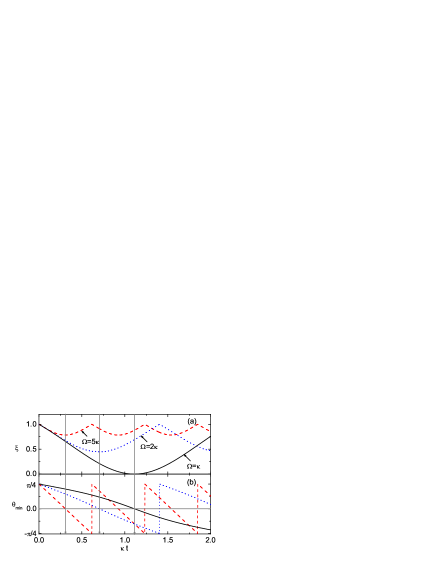
Figure 1: (color online) Time evolution of (a) the squeezing parameter and (b) the squeezing angle for $N=2$ and various Rabi frequencies: $\Omega=5\kappa$ (Dashed red lines), $\Omega=2\kappa$ ( Dotted blue lines), and $\Omega=\kappa$ (Solid black lines). The maximal-squeezing times $t_{0}$ for different $\Omega$ are indicated by the vertical lines.

In Fig. 1, time evolutions of $\xi$ and $\theta_{\min}$ are investigated for the coupling $\Omega\geq\kappa$. We observe that local minima of $\xi$ together with $\theta_{\min}=0$ also occurs periodically at the times $t_{k}$. Moreover, with the decrease of $\Omega$, the squeezing parameter at $t_{k}$ becomes small, i.e., more squeezed. For the coupling $\Omega=\kappa$, the spin system is optimally squeezed at $t_{k}$, as shown by the solid black lines of Fig. 1. In this case $\sin(\eta)=\cos(\eta)=1/\sqrt{2}$, and the spin states at $t_{k}$ are

$$|\psi(t_{k})\rangle = (-1)^{k}\frac{ie^{-i\kappa t_{k}}}{\sqrt{2}}\left\{\left|1,-1\right\rangle_{x}-\left|1,+1\right\rangle_{x}\right\}$$ (11)

$$= i(-1)^{k+1}e^{-i\kappa t_{k}}|j=1,m=0\rangle.$$

Here, the state $(|1,-1\rangle_{x}-|1,+1\rangle_{x})/\sqrt{2}$ is maximally entangled (or Bell) state, while the Dicke state $|j=1,m=0\rangle$ is maximally squeezed state Wineland . For this state, both the mean spin $\langle\hat{J}_{x}\rangle$ and the variance $(\Delta\hat{J}_{\mathbf{n}})_{\min}$ are equal to zero, which makes it hard to define $\xi$ as Eq. (1). To avoid this problem, Wineland et al. proposed another definition of the squeezing parameter, namely $\xi\rightarrow(j/|\langle\hat{J}\rangle|)\xi$, which gives the smallest squeezing $1/\sqrt{2}$ for $N=2$ case Wineland .

III.2 Three-particle case

For $N=3$ ($j=3/2$) case, we introduce the linear combinations of the amplitudes $p_{m}^{(+)}(t)=c_{m}(t)+c_{-m}(t)$ with $m=1/2,3/2$. Since $p_{3/2}^{(+)}(0)=p_{1/2}^{(+)}(0)=0$, we get $p_{m}^{(+)}(t)=0$. Therefore, the amplitudes obey $c_{m}(t)=-c_{-m}(t)$, from which we can prove that the mean spin is always along the $x$ direction. Such result keeps valid for any odd $N$ case. From Eq. (3), we obtain a coupled equations for the linear combinations $p_{m}^{(-)}(t)=c_{m}(t)-c_{-m}(t)$:

$$i\left(\begin{array}[]{c}\dot{p}_{1/2}^{(-)}\\ \dot{p}_{3/2}^{(-)}\end{array}\right)=\left(\begin{array}[]{cc}E^{\prime}_{1/2}&X_{3/2}\\ X_{3/2}&E_{3/2}\end{array}\right)\left(\begin{array}[]{c}p_{1/2}^{(-)}\\ p_{3/2}^{(-)}\end{array}\right),$$ (12)

where $E^{\prime}_{1/2}=E_{1/2}-X_{1/2}$. The initial conditions are $p_{3/2}^{(-)}(0)=-1/\sqrt{2}$ and $p_{1/2}^{(-)}(0)=\sqrt{3/2}$. Dynamical evolution of the three-spin system is determined solely by Eq. (12). The analytic expression of the variance is

$$(\Delta\hat{J}_{\mathbf{n}})_{\min}^{2} = \frac{3}{4}+\frac{3\kappa^{2}}{S^{2}}\sin^{2}St$$ (13)

$$-\frac{3\kappa}{S}\left|\sin St\right|\sqrt{1-\frac{3\kappa^{2}}{S^{2}}\sin^{2}St},$$

and the squeezing angle is

$$\theta_{\min}=\frac{1}{2}\tan^{-1}\left[\frac{S\cos(St)}{(\Omega+\kappa)\sin(St)}\right],$$ (14)

where $2S=\mathcal{E}_{3}-\mathcal{E}_{1}=2\sqrt{\Omega^{2}+2\kappa\Omega+4\kappa^{2}}$ is the level spacing for $N=3$ case, and $\mathcal{E}_{3}$ and $\mathcal{E}_{1}$ correspond to two eigenvalues of the coefficient matrix of Eq. (12).

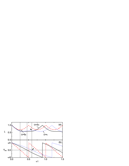
Figure 2: (Color online) Time evolution of (a) the squeezing parameter, and (b) the squeezing angle for $N=3$ case with various Rabi frequencies: $\Omega=5\kappa$ (Dashed red lines), $\Omega=2\kappa$ (Solid black lines), and $\Omega=\kappa$ (Dotted blue lines).

In Fig. 2, we investigate time evolution of $\xi$ and $\theta_{\min}$ for $N=3$ case. Similar with previous $N=2$ case, our results show that for $\Omega\geq 2\kappa$, local minima of $\xi$ together with $\theta_{\min}=0$ also occur at the times $St_{k}=(k+1/2)\pi$. As shown by the solid black line of Fig. 2, we find that the optimal squeezing can be obtained at $t_{k}$ for the coupling $\Omega=2\kappa$. The maximally squeezed state at $t_{k}$ reads

$$|\psi(t_{k})\rangle=\frac{i(-1)^{k}}{\sqrt{2}}e^{-3i\kappa t_{k}/2}\left(\left|\frac{3}{2},\frac{1}{2}\right\rangle-\left|\frac{3}{2},-\frac{1}{2}\right\rangle\right).$$ (15)

Such a state gives the smallest squeezing parameter $\xi(t_{k})=1/\sqrt{3}$ that the three-particle system can reach. It is worth mentioning that for $\Omega<2\kappa$, the vanishing $\theta_{\min}$ appearing at $t_{k}$ no longer corresponds to local minima of $\xi$, as shown by the dotted blue lines of Fig. 2. The time scale $t_{k}$ is relevant to determine the MST only for $\Omega$ equal or larger than the optimal coupling.

In short, we find some basic features for two exactly solvable cases. Local minima of $\xi$ with $\theta_{\min}=0$ occur at the MST $t_{k}$. This is no longer true if $\Omega$ smaller than the optimal coupling. The time scale $t_{k}$ depends on the level spacing $2S$ between the ground state and the second excited state. Due to the symmetric properties of the spin system, the first excited eigenstate is an idle level (see below). This is also the reason why we can introduce the linear combinations of the amplitudes $p_{m}^{(\pm)}$, with $m=0,1$ for $N=2$, and $m=1/2,3/2$ for $N=3$. For the optimal coupling, the spin system will be evolved into the maximally squeezed state at $t_{k}$ : $|1,0\rangle$ (for $N=2$) or $(|3/2,1/2\rangle-|3/2,-1/2\rangle)/\sqrt{2}$ (for $N=3$), which is just the ground state of $2\kappa\hat{J}_{z}^{2}$. We will extend the above results to many-particle cases.

IV Many-particle cases: The maximal-squeezing time

In this section, we study the spin squeezing for many-particle cases focusing on the time scale of the maximal squeezing. For instance, we consider the spin system with particle number $N=40$ Kitagawa ; Takeuchi . The numerical results are shown in Fig. 3. We find that with the increase of $\Omega$, the squeezing $\xi$ and the mean spin $\langle\hat{J}_{x}\rangle$ show collapsed oscillations Agarwal ; Jin04 . Local maxima of the mean spin $\langle\hat{J}_{x}\rangle$ always appear together with the vanishing $\theta_{\min}$. We can prove this from Heisenberg equation of $\hat{J}_{x}$ and Eq. (5): $d\langle\hat{J}_{x}\rangle/dt\sim\langle\hat{J}_{z}\hat{J}_{y}+\hat{J}_{y}\hat{J}_{z}\rangle\sim A\tan(2\theta_{\min})$. If the mean spin reaches its local maximum at a certain time $t_{0}$, then $\left.d\langle\hat{J}_{x}\rangle/dt\right|_{t_{0}}=0$, which leads to $\theta_{\min}=0$ at $t_{0}$ provided that $A\neq 0$.

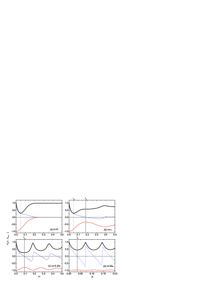
Figure 3: (color online) Time evolution of $\xi$ (thick solid lines), $\theta_{\min}$ (dashed blue lines) and $\langle\hat{J}_{x}\rangle/j$ (thin red lines) for $N=40$ ($j=20$) and various Rabi frequencies: (a) $\Omega=0$, (b) $\Omega=\kappa$, (c) $\Omega=4.24\kappa$ (the optimal coupling), and (d) $\Omega=20\kappa$. The time scale $t_{0}$ for different $\Omega$ are indicated by the vertical lines.

As shown in Fig. 3(b), for a small coupling with $\Omega=\kappa$, there are two time scales: $t_{0}$ for the vanishing $\theta_{\min}$, and $\tau_{0}$ for the maximal squeezing. Note that the latter time scale $\tau_{0}$ closes to that of the OAT result ($\Omega=0$ case), i.e. $\kappa\tau_{0}\simeq 0.04986$. With the increase of $\Omega$, these two time scales become coincident, as shown in Fig. 3(c) and (d). Unlike to the exactly solvable cases, we find that the optimal coupling for $N=40$ is not a fixed value but can be arbitrary $\Omega$ in a region $4.239\leq\Omega_{R}/\kappa\leq 4.242$. Fig. 3(c) represents the optimal squeezing case with the coupling $\Omega=4.24\kappa$. Starting from the initial CSS, the spin system evolves into the maximally squeezed state at $\kappa t_{0}=0.09$.

To investigate the maximally SSS at $t_{0}$, we calculate the quasiprobability distribution (QPD, or the Husimi function) $Q(\theta,\phi)$ on the Bloch sphere Kitagawa

$$Q(\theta,\phi)=|\langle\theta,\phi|\psi(t)\rangle|^{2},$$ (16)

where $|\theta,\phi\rangle=\exp\{-i\theta(\hat{J}_{x}\sin\phi-\hat{J}_{y}\cos\phi)\}|j,-j\rangle$ is the generalized coherent spin state CSS1 ; CSS2 . The initial state is a particular case of the CSS, namely $|j,-j\rangle_{x}=|\theta=\pi/2,\phi=\pi\rangle$. The QPD can be used to simulate the variation of spin uncertainties. The circle in Fig. 4(a) represents an isotropic spin variance for the initial CSS, while the shaded ellipse parts in Fig. 4(b) and (c) are that of the SSS at times about $t_{0}/2$ and $t_{0}$, respectively. Unlike to the OAT result Kitagawa ; Takeuchi , the maximal variance reduction appears along the $z$ axis with $\theta_{\min}=0$ Law . In Fig. 4, we also calculate the probability distribution $|c_{m}|^{2}=|\langle j,m|\psi(t)\rangle|^{2}$ of the spin state for $N=40$ and the optimal coupling $\Omega=4.24\kappa$. Compared with the initial CSS, we find that the maximally SSS at $t_{0}$ has a very sharp probability distribution with a large amplitude of the lowest spin projection, i.e., $m=0$ (for even $N$) or $m=\pm 1/2$ (for odd $N$) LW10041 . Such a sharp probability distribution of the SSS can be explained qualitatively by considering the familiar phase model phase model (see also references therein).

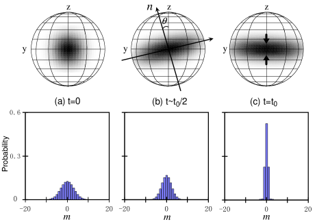
Figure 4: Time evolution of the quasiprobability distribution $Q(\theta,\phi)$ (top) and the probability distribution $|c_{m}|^{2}$ (bottom) at the times (a) $\kappa t=0$, (b) $\kappa t=0.04$, and (c) $\kappa t=0.09$ (the MST). The QPD is normalized such that $Q(\pi/2,\pi)=1$. In (b), the spin component normal to the $x$ axis is defined as $\hat{J}_{\mathbf{n}}=\hat{J}\cdot\mathbf{n}$ with $\mathbf{n}=(0,\sin\theta,\cos\theta)$. Other parameters are taken as those of Fig. 3(c).

In order to determine the time scale $t_{0}$, we employ numerical diagonalization of the Hamiltonian (2) to obtain a set of eigenenergies $\{\mathcal{E}_{n};n=1,2,3,...\}$, where $n=1$ denotes the ground state, $n=2$ the first excited state, and $n=3$ the second excited state, etc., thus

$$\hat{H}|\phi_{n}\rangle=\mathcal{E}_{n}|\phi_{n}\rangle,$$ (17)

where $\mathcal{E}_{n}$ and $|\phi_{n}\rangle$ with $n=1,2,3,\cdots,(2j+1)$ depend on the parameters $N$ and $\Omega$ Note . As shown in Fig. 5(a), we plot parts of $\mathcal{E}_{n}$ for $j=20$ ($N=40$) as a function of the coupling $\Omega$. Similar with previous two- and three-particle cases, we suppose that the MST $t_{0}$ depends on the level spacing between $n=1$ and $n=3$, namely $t_{0}=\pi/(2S)$ with $2S=\mathcal{E}_{3}-\mathcal{E}_{1}$. To check it, in Table 1, we compare exactly numerical results of the time $t_{0}$ with $\pi/(2S)$ for various $N$ and $\Omega$. Our diagonalization method gives accurate prediction of the time $t_{0}$. We remark that for $N=2$ and $N=3$ cases, both two results are exactly the same.

Table 1: Comparison of exactly numerical $t_{0}$, $\pi/(2S)$, and analytic results of Eq. (18) for different $N$ and $\Omega$. The times are in units of $(100\kappa)^{-1}$.

		$N=40$			$N=200$			$N=1000$
$\Omega/\kappa$:	1	4.24	20	1	6.7	25	1	10.8	50
Exact num.	18.28	9.065	3.604	8.192	3.184	1.549	3.665	1.104	0.4945
$\pi/(2S)$	19.02	8.615	3.573	8.143	3.048	1.533	3.571	1.071	0.4916
Eq. (18)	17.56	8.529	3.927	7.854	3.034	1.571	3.512	1.069	0.4967

To explain the above agreements, we calculate the spectral distribution of the spin state, i.e., $|\langle\phi_{n}|\psi(t)\rangle|^{2}$ in Fig. 5(b)-(d) for $N=40$ and various $\Omega$. Physically, the spectral distribution measures the population distribution of the state vector $|\psi(t)\rangle$ on the eigenstates $|\phi_{n}\rangle$ MZI . For fixed parameters $N$ and $\Omega$, the spectral distribution $|\langle\phi_{n}|\psi(t)\rangle|^{2}$ is time-independent. In fact, one can expand the spin state in terms of $\{|\phi_{n}\rangle\}$: $|\psi(t)\rangle=\sum_{n}d_{n}(t)|\phi_{n}\rangle$ with the amplitudes $d_{n}(t)=\exp[-i\mathcal{E}_{n}t]d_{n}(0)$. Here the initial amplitudes $d_{n}(0)$ depend only on the initial condition Eq. (4), therefore the spectral distribution $|\langle\phi_{n}|\psi(t)\rangle|^{2}=|d_{n}(t)|^{2}\equiv|d_{n}(0)|^{2}$ and is time-independent for fixed $N$ and $\Omega$. From our numerical calculations, Fig. 5(b-d), we find that total occupation of the spin state $|\psi(t)\rangle$ on the eigenstates $n=1$ and $n=3$ is over $80$ percent. This is the reason why the MST depends on the level spacing between these two levels. Moreover, we find the even $n$ eigenstates are in fact the idle levels, just as previous $N=2$ and $N=3$ cases.

Except for $N=2$ and $N=3$, exact solutions for the nonlinear spin system within the small-coupling regime ($1<\Omega/\kappa<<N$) do not exist Law ; Agarwal . In our previous work LW10041 , however, we have obtained the analytic expression of the MST based upon the phase model:

$$\kappa t_{0}\simeq\frac{\pi}{2}\sqrt{\frac{\kappa}{2\Omega N}},$$ (18)

which is valid for large $N$ ($\geq 10^{3}$). Our analytic solution of the MST is derived by the prediction $t_{0}\simeq T/4$, where $T=2\pi/\omega_{\text{eff}}$ is the period of the pendulum near the bottom of a periodic potential LW10041 . In fact, for large $N$ the spin system behaviors as a pendulum rotating with the oscillating frequency $\omega_{\text{eff}}=\sqrt{2\kappa\Omega_{R}N}$. As shown in Table 1, we compare $\pi/(2S)$, the analytic solutions of Eq. (18), and the exact numerical results of the MST for various parameters $\Omega$ and $N$. It is shown that our analytical expression of Eq. (18) works very well for the large $N$ ($\sim 10^{3}$), which implies that the oscillating frequency $\omega_{\text{eff}}$ has its physical meaning to be half of the level spacing $S=(\mathcal{E}_{3}-\mathcal{E}_{1})/(2\hbar)$. Note that the phase model or Eq. (18) is valid for the large $N$, while $\pi/(2S)$ is no limited by this. From this sense, we believe that the diagonalization method presented here provides much comprehensive way to measure the maximal-squeezing time.

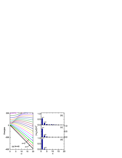
Figure 5: (color online) (a) Part of the Eigenenergies $\mathcal{E}_{n}$ as a function of $\Omega$ for $N=40$. The spectral distribution $|\langle\phi_{n}|\psi(t)\rangle|^{2}$ for (b) $\Omega=\kappa$, (c) $\Omega=4.24\kappa$, and (d) $\Omega=20\kappa$.

V CONCLUSIONS

In summary, we have studied the maximal-squeezing time of a nonlinear spin system, which can be realized in the two-component BEC, or other spin system similar with Takeuchi et al.Takeuchi . Motivated by two exactly solvable cases for $N=2$ and $N=3$, we show that time scale of the maximal squeezing depends on the level spacing between $n=1$ and $n=3$ eigenstates. We explain it by calculating the probability distribution of the spin state on the eigenstates of the Hamiltonian, and find that the above two states are occupied predominantly. Such results keep valid for arbitrary $N$ and a wide rage of the coupling strength.

- (1) Present address: Department of physics, School of Science, Beijing Jiaotong University, Beijing 100044, China
- (2) Electronic address: swkim0412@pusan.ac.kr
- (3) M. Kitagawa and M. Ueda, Phys. Rev. A 47, 5138 (1993).
- (4) D. J. Wineland, J. J. Bollinger, W. M. Itano, F. L. Moore, and D. J. Heinzen, Phys. Rev. A 46, R6797 (1992); ibid. 50, 67 (1994).
- (5) Q.A. Turchette, C.S. Wood, B.E. King, C.J. Myatt, D. Leibfried, W.M. Itano, C. Monroe and D.J. Wineland. Phys. Rev. Lett. 81, 3631 (1998).
- (6) V. Meyer et al., Phys. Rev. Lett. 86, 5870 (2001).
- (7) D. Leibfried et al., Science 304, 1476 (2004).
- (8) A. Kuzmich, K. Molmer, and E.S. Polzik, Phys. Rev. Lett. 79, 4782 (1997).
- (9) J. Hald, J. L. Sørensen, C. Schori, and E. S. Polzik, Phys. Rev. Lett. 83, 1319 (1999).
- (10) J. M. Geremia, J. K. Stockton, and H. Mabuchi, Science 304, 270 (2004).
- (11) A. G. Rojo, Phys. Rev. A, 68, 013807 (2003).
- (12) A. Sørensen, L. M. Duan, I. Cirac, and P. Zoller, Nature (London) 409, 63 (2001).
- (13) K. Helmerson and L. You, Phys. Rev. Lett. 87, 170402 (2001); Ö.E. Müstecaplioğlu, M. Zhang, and L. You, Phys. Rev. A 66, 033611 (2002); M. Zhang et al., Phys. Rev. A 68, 043622 (2003).
- (14) X. Wang and B. C. Sanders, Phys. Rev. A 68, 012101 (2003).
- (15) J. K. Korbicz, J. I. Cirac, and M. Lewenstein, Phys. Rev. Lett. 95, 120502 (2005); J. K. Korbicz, O. Gühne, M. Lewenstein, H. Häffner, C.F. Roos, and R. Blatt, Phys. Rev. A 74, 052319 (2006) .
- (16) S. Yi and H. Pu, Phys. Rev. A 73, 023602 (2006).
- (17) U. V. Poulsen and K. Molmer, Phys. Rev. A 64, 013616 (2001).
- (18) M. Takeuchi et al., Phys. Rev. Lett. 94, 023003 (2005).
- (19) D. Jaksch, J. I. Cirac, and P. Zoller, Phys. Rev. A 65, 033625 (2002).
- (20) C.K. Law, H.T. Ng, and P.T. Leung, Phys. Rev. A 63, 055601 (2001).
- (21) S. Raghavan, H. Pu, P. Meystre, and N. P. Bigelow, Opt. Commu. 188, 149 (2001).
- (22) S. D. Jenkins et al., Phys. Rev. A 66, 043621 (2002).
- (23) S. Choi and N. P. Bigelow, Phys. Rev. A 72, 033612 (2005).
- (24) Z. -D. Chen, J. -Q. Liang, S. -Q. Shen, and W. -F. Xie, Phys. Rev. A 69, 023611 (2004).
- (25) G. J. Milburn et al., Phys. Rev. A 55, 4318 (1997); G. L. Salmond et al., ibid. 65, 033623 (2002).
- (26) A. Smerzi, S. Fantoni, S. Giovanazzi, and S. R. Shenoy, Phys. Rev. Lett. 79, 4950 (1997); S. Raghavan, A. Smerzi, S. Fantoni, S. R. Shenoy, Phys. Rev. A, 59, 620 (1999).
- (27) P. Villain, M. Lewenstein, R. Dum, Y. Castin, L. You, A. Imamoglu and T.A.B. Kennedy, J. Mod. Opt. 44, 1775 (1997).
- (28) J.I. Cirac, M. Lewenstein, K. Molmer, and P. Zoller, Phys. Rev. A 57, 1208 (1998).
- (29) M.J. Steel and M.J. Collett, Phys. Rev. A 57, 2920 (1998).
- (30) E. M. Wright, D. F. Walls, and J. C. Garrison, Phys. Rev. Lett. 77, 2158 (1996); E. M. Wright et al., Phys. Rev. A 56, 591 (1997).
- (31) D. Gordon and C. M. Savage, Phys. Rev. A 59, 4623 (1999).
- (32) L. M. Kuang and Z. W. Ouyang, Phys. Rev. A 61, 023604 (2000); L. M. Kuang and L. Zhou, ibid 68, 043606 (2003).
- (33) D. S. Hall et al., Phys. Rev. Lett. 81, 1539 (1998); idib, 1543 (1998).
- (34) J. Stenger et al., Nature 396, 345 (1998).
- (35) G. S. Agarwal and R. R. Puri, Phys. Rev. A 39, 2969 (1989).
- (36) L. Zhou, H. S. Song, and C. Li, J. Opt. B: Quantum Semiclassical Opt. 4, 425 (2002).
- (37) E. Hagley, X. Maitre, G. Nogues, C. Wunderlich, M. Brune, J.-M. Raimond and S. Haroche. Phys. Rev. Lett. 79, 1 (1997).
- (38) A. Messikh, Z. Ficek, and M. R. B. Wahiddin, Phys. Rev. A 68, 064301 (2003).
- (39) B. Zeng, D. L. Zhou, Z. Xu, and L. You, Phys. Rev. A 71, 042317 (2005).
- (40) G. R. Jin and W. M. Liu, Phys. Rev. A 70, 013803 (2004); G. R. Jin, Z. X. Liang, and W. M. Liu, J. Opt. B: Quantum Semiclass. Opt. 6, 296 (2004).
- (41) J. M. Radcliffe, J. Phys. A 4, 313 (1971).
- (42) F. T. Arecchi, E. Courtens, R. Gilmore, and H. Thomas, Phys. Rev. A 6, 2211 (1972).
- (43) G. R. Jin and S. W. Kim, to be appeared in Phys. Rev. Lett., (2007).
- (44) D. Jaksch, S. A. Gardiner, K. Schulze, J. I. Cirac, and P. Zoller, Phys. Rev. Lett. 86, 4733 (2001); C. Menotti, J. R. Anglin, J. I. Cirac, and P. Zoller, Phys. Rev. A 63, 023601 (2001); A. Micheli et al., ibid. 67, 013607 (2003).
- (45) Except Table I, we choose a fixed scatting strength throughout our paper, so the time scale is in units of .
- (46) C. Lee, Phys. Rev. Lett. 97, 150402 (2006).