On rough isometries of Poisson processes on the line

Abstract

Intuitively, two metric spaces are rough isometric (or quasi-isometric) if their large-scale metric structure is the same, ignoring fine details. This concept has proven fundamental in the geometric study of groups. Abért, and later Szegedy and Benjamini, have posed several probabilistic questions concerning this concept. In this article, we consider one of the simplest of these: are two independent Poisson point processes on the line rough isometric almost surely? Szegedy conjectured that the answer is positive.

Benjamini proposed to consider a quantitative version which roughly states the following: given two independent percolations on $\mathbb{N}$, for which constants are the first $n$ points of the first percolation rough isometric to an initial segment of the second, with the first point mapping to the first point and with probability uniformly bounded from below? We prove that the original question is equivalent to proving that absolute constants are possible in this quantitative version. We then make some progress toward the conjecture by showing that constants of order $\sqrt{\log n}$ suffice in the quantitative version. This is the first result to improve upon the trivial construction which has constants of order $\log n$. Furthermore, the rough isometry we construct is (weakly) monotone and we include a discussion of monotone rough isometries, their properties and an interesting lattice structure inherent in them.

1 Introduction

The concept of rough isometry (sometimes also called quasi-isometry or coarse quasi-isometry) of two metric spaces was introduced by Kanai in K85 and, in the more restricted setting of groups, by Gromov in G81 . Informally, two metric spaces are rough isometric if their metric structure is the same up to multiplicative and additive constants. This allows stretching and contracting of distances, as well as having many points of one space mapped to one point of the other. For example, $R^{d}$ and $\mathbb{Z}^{d}$ are rough isometric. This concept has proven fundamental in the geometric study of groups. On the one hand, the rough isometry concept is stringent enough to preserve some of the metric properties of the underlying space. On the other hand, it is loose enough to allow for large equivalence classes of spaces. For example, rough isometry preserves (under some conditions) geometric properties of the space such as volume growth and isoperimetric inequalities K85 . It preserves analytic properties such as the parabolic Harnack inequality D99 (and also K05 , Section 2.1) and, in a more probabilistic context, various estimates on transition probabilities of random walks (heat kernel estimates) are preserved; again, see K05 , Section 2, and the references contained therein. Formally, we have the following.

Definition 1.1.

Two metric spaces $X$ and $Y$ are rough isometric (or quasi-isometric) if there exists a mapping $T\dvtx X\to Y$ and constants $M,D,R\geq 0$ such that:

any $x_{1},x_{2}\in X$ satisfy

$$\frac{1}{M}d_{X}(x_{1},x_{2})-D\leq d_{Y}(T(x_{1}),T(x_{2}))\leq Md_{X}(x_{1},x_{2})+D;$$

for any $y\in Y$, there exists some $x\in X$ such that $d_{Y}(y,T(x))\leq R$.

The first condition ensures that the metric is not distorted too much multiplicatively or additively; the second condition implies that the map is close to being onto. On first inspection, it appears that the definition is not symmetric in $X$ and $Y$, but one may easily check that if such a mapping $T\dvtx X\to Y$ exists, then another mapping $\widetilde{T}\dvtx Y\to X$ also exists, satisfying the same conditions, with the roles of $X$ and $Y$ interchanged (and with possibly different constants).

We will sometimes abbreviate “rough isometric” to “r.i.”

In this article, we are concerned with an aspect of the question of how large the equivalence classes of rough isometric spaces are. We investigate this question in a probabilistic setting. Specifically Miklós Abért asked in 2003 A03 whether, for a finitely generated group, two infinite clusters of independent edge percolations on its Cayley graph are rough isometric almost surely (assuming they exist). In this generality, the question appeared difficult and so Balázs Szegedy suggested considering whether two site percolations on $\mathbb{Z}^{2}$ are rough isometric (disregarding connectivity properties). When this also appeared difficult, he suggested considering the case of $\mathbb{Z}$. These questions have since remained open. Independently, and a short time later, the $\mathbb{Z}^{d}$ questions were also raised by Itai Benjamini (following the related work AB03 ) who also introduced a quantitative variant. The one-dimensional question is easily seen to be equivalent to the following (see Proposition 2.2 below): are two independent Poisson processes on the line (viewed as random metric spaces with their metric inherited from $\mathbb{R}$) rough isometric a.s.? Szegedy conjectured a positive answer to this question.

This question is a form of matching problem, but, unlike some other matching problems in which we wish to minimize some quantity on average, or to have it bounded for most points, here, we need to satisfy the rigid constraints of a rough isometry for all points. To our aid comes the fact that the Poisson processes are infinite and we may “start” constructing the rough isometry at a particularly convenient location and use the freedom afforded by large constants to “plan ahead.” Unfortunately, this article does not settle this conjecture, but it makes some modest progress. In the next section, we prove the equivalence of the problem to several other related problems involving percolations on the integers and on the natural numbers, including Benjamini’s quantitative variant. Our main result is the construction of a monotone rough isometry with certain properties giving a first nontrivial upper bound on the quantitative variant. Section 3 presents a discussion of monotone rough isometries, their properties and an interesting lattice structure inherent in them. As noted there, in general, monotone rough isometries between subsets of $\mathbb{Z}$ are more restrictive than general rough isometries. In particular, it may be harder to find a monotone rough isometry between two independent Poisson processes than to find a general rough isometry. Section 4 contains the proofs of all the theorems in Section 2, except for the main construction. Section 5 presents the main construction.

2 Versions of the problem and main result

In this section, we will first state in precise terms the main open question described in the Introduction. We will then proceed to show the equivalence of the question to several other related problems. We shall go from the continuous Poisson process question to a discrete variant (percolation on $\mathbb{Z}$), then to an oriented discrete variant (percolation on $\mathbb{N}$) and, finally, to a finite variant (percolation on an initial segment of $\mathbb{N}$), all of which are equivalent. We will then state a quantitative version of our main open question (due to Benjamini), based on the finite variant, and conclude the section with a statement of our main result which gives the first nontrivial upper bound on this quantitative version. The proofs of all statements in this section, except for the main result, are presented in Section 4; the proof of the main result is presented in Section 5.

Proposition 2.1.

Given two independent Poisson processes $A,B\subseteq\mathbb{R}$ (possibly of different intensities) and constants $(M,D,R)$, the event that $A$ and $B$ are rough isometric with constants $(M,D,R)$ is a zero-one event.

Hence, we come to the following question.

Main Open Question 1.

Do there exist constants $(M,D,R)$ for which two independent Poisson processes of intensity 1 are rough isometric a.s.?

In this article, we shall mostly consider a discrete variant of the question involving Bernoulli percolations on $\mathbb{Z}$ or on $\mathbb{N}$, rather than Poisson processes. We remind the reader that a Bernoulli percolation on $\mathbb{Z}$ with parameter $p$ is the random subset $A\subseteq\mathbb{Z}$ obtained from $\mathbb{Z}$ by independently deleting each integer with probability $1-p$. It is defined analogously for $\mathbb{N}$. The next proposition states the equivalence of the problem for Bernoulli percolations and for Poisson processes.

Proposition 2.2.

The following are equivalent:

for some intensities $\alpha,\beta>0$, two independent Poisson processes, one with intensity $\alpha$ and the other with intensity $\beta$, are rough isometric a.s.;

for any intensities $\alpha,\beta>0$, two independent Poisson processes, one with intensity $\alpha$ and the other with intensity $\beta$, are rough isometric a.s.;

for some $0<p,q<1$, two independent Bernoulli percolations on $\mathbb{Z}$, one with parameter $p$ and the other with parameter $q$, are rough isometric a.s.;

for any $0<p,q<1$, two independent Bernoulli percolations on $\mathbb{Z}$, one with parameter $p$ and the other with parameter $q$, are rough isometric a.s.

Since, by the previous proposition, we may equivalently consider any intensity for the Poisson process and any parameter for Bernoulli percolation, we fix notation and, from this point on, consider only Poisson processes with unit intensity and Bernoulli percolations with parameter $\frac{1}{2}$.

A rough isometry between two Poisson processes or between two Bernoulli percolations on $\mathbb{Z}$ is not necessarily order preserving (or order reversing), as will be discussed in more detail near the end of this section. Still, one feels intuitively that such a mapping should be monotonic in some rough sense. Indeed, for the next two theorems, we will need to show that such a mapping is at least “almost monotonic at most points,” in a sense made precise in the following statements and their proofs. We start by showing that a certain oriented version of the problem is equivalent to the original problem. For this purpose, we introduce the following new concept.

Definition 2.1.

Two rooted metric spaces $(X,a)$ and $(Y,b)$ are rooted rough isometric if there exists a mapping $T\dvtx X\to Y$ and constants $M,D,R\geq 0$ such that $T(a)=b$ and the conditions in the usual definition of rough isometry hold for $T$ and the constants $(M,D,R)$.

We also introduce a different random model, as follows.

Definition 2.2.

A rooted Bernoulli percolation on $\mathbb{N}$ (with parameter $\frac{1}{2}$) is a random subset $A\subseteq\mathbb{N}\cup\{0\}$ in which $0\in A$ deterministically and any $n\in\mathbb{N}$ belongs to $A$ with probability $\frac{1}{2}$ independently.

Theorem 2.3.

The following are equivalent:

two independent Bernoulli percolations on $\mathbb{Z}$ (with parameter $\frac{1}{2}$) are rough isometric a.s.;

two independent rooted Bernoulli percolations $(A,0)$ and $(B,0)$ on $\mathbb{N}$ are rooted rough isometric with positive probability.

To prove this theorem, we need the following definition.

Definition 2.3.

Given two subsets $A,B\subseteq\mathbb{Z}$ and a mapping $T\dvtx A\to B$, the point $x\in A$ is called a cut point for $T$ if one of the following occurs:

1. [($\alpha$)]

2. for all $z\in A$ with $z>x$, we have $T(z)\geq T(x)$;

3. for all $z\in A$ with $z>x$, we have $T(z)\leq T(x)$.

We also require the following lemma.

Lemma 2.4.

If two independent Bernoulli percolations on $\mathbb{Z}$ are rough isometric a.s. with constants $(M,D,R)$, then, with probability 1, any rough isometry $T\dvtx A\to B$ with constants $(M,D,R)$ has a cut point.

We continue to construct a finite variant of our problem. First, we define, for a given infinite subset $A\subseteq\mathbb{N}\cup\{0\}$, $A(n)\subseteq A$ to be its first $n$ points [e.g., if $A=(0,1,3,4,6,\ldots)$, then $A(3)=(0,1,3)$]. Also, given $A,B\subseteq\mathbb{N}\cup\{0\}$ both containing $0$, we sometimes say that $A(n)$ is rooted r.i. to some initial segment of $B$ if there exists an $m$ and a rooted r.i. $T\dvtx A(n)\to B(m)$. We may also phrase this as $T$ is a rooted r.i. of $A(n)$ to some initial segment of $B$. We now have the following result.

Theorem 2.5.

The following are equivalent:

two independent rooted Bernoulli percolations $(A,0)$ and $(B,0)$ on $\mathbb{N}$ are rooted rough isometric with positive probability;

there exists some $p>0$ and constants $(M,D,R)$ such that, given two independent rooted Bernoulli percolations $(A,0)$ and $(B,0)$ on $\mathbb{N}$, for any $n\geq 1$, $A(n)$ is rooted r.i. to some initial segment of $B$ with constants $(M,D,R)$ and with probability at least $p$.

Although this theorem may initially seem straightforward, it transpires that the direction $\mbox{(i)}\to\mbox{(ii)}$ is somewhat problematic. The main difficulty stems from the fact that, given a rooted rough isometry from $A\subseteq\mathbb{N}\cup\{0\}$ to $B\subseteq\mathbb{N}\cup\{0\}$, its restriction to $A(n)$ is not necessarily a rooted rough isometry to some $B(m)$ with the same constants. This is due to the fact that a rough isometry need not be monotonic and hence the image of its restriction to $A(n)$ may still have big “holes” [i.e., points $b\in B$ where property (ii) in the definition of rough isometry does not hold] which are “filled” by the mapping at subsequent points of $A$. To prove this theorem, we will need a statement asserting that if $A$ and $B$ are rooted Bernoulli percolations, then $T\dvtx A\to B$ is a rooted rough isometry with constants $(M,D,R)$, and if we allow the constant $R$ to be increased sufficiently, say to some $L:=L(M,D,R)$, then for “most $n$’s” the restriction of $T$ to $A(n)$ will still be a rooted rough isometry to some initial segment of $B$ with constants $(M,D,L)$. This is the content of the next three lemmas: they make precise what was meant when we stated previously that a rough isometry is “almost monotonic at most points.”

We now introduce the following notation: given $A\subseteq\mathbb{N}\cup\{0\}$ and $x\in A$, let $\operatorname{Succ}(x)$ be the smallest point in $A$ which is larger than $x$ (or $\infty$ if there is no such point) and let $\operatorname{Gap}(x):=\operatorname{Succ}(x)-x$. We start with a deterministic lemma.

Lemma 2.6.

Let $A,B\subseteq\mathbb{N}\cup\{0\}$ be infinite subsets, both containing $0$, and let $T\dvtx A\to B$ be a rooted r.i. between them with constants $(M,D,R)$. There exists $L:=L(M,D)$ such that if there exist $x,y\in A$ with $x<y$ and $T(y)\leq T(x)-L$, then there exists $z\in A$, $z\geq y$ and $z-x\geq\frac{L}{2M}$ such that $\operatorname{Gap}(z)\geq\frac{z-x}{2M^{2}}$.

We continue with a probabilistic aspect of the previous lemma.

Lemma 2.7.

Let $A$ be a rooted Bernoulli percolation on $\mathbb{N}$, let $w\in\mathbb{N}$ and define, for constants $L,M$, the event $E^{w}_{L,M}:=\{\exists z\in A,z>w,\operatorname{Gap}(z)\geq\max(\frac{L}{4M^{3}},\frac{z-w}{2M^{2}})\}$. Then $\mathbb{P}(E^{w}_{L,M})\leq C(\frac{L}{M}+1)e^{-c{L}/{M^{3}}}$ for some absolute constants $C,c>0$ (not depending on any parameter).

Finally, we have one more deterministic lemma.

Lemma 2.8.

Let $A,B\subseteq\mathbb{N}\cup\{0\}$ be infinite subsets, both containing $0$, and let $T\dvtx A\to B$ be a rooted r.i. between them with constants $(M,D,R)$. Fix $L>R$ and $n\geq 1$, let $x_{n}$ be the $n$th point of $A$ and suppose that the event $E^{x_{n}}_{L-R,M}$ of Lemma 2.7 does not hold for $A$. Then $T$ restricted to $A(n)$ is a rooted r.i. of $A(n)$ to $B(m)$ for some $m$ with constants $(M,D,L)$.

Remark 2.1.

Close inspection of the proof of part $\mbox{(ii)}\to\mbox{(i)}$ of Theorem 2.5 reveals that (ii) is, in fact, equivalent (by the same proof) to the following, seemingly weaker, statement [the $R$-denseness property is property (ii) in the definition of r.i.]:

(iii) There exists $p>0$, constants $(M,D,R)$ and a function $f(n)\to\infty$ such that given two independent rooted Bernoulli percolations $(A,0)$ and $(B,0)$ on $\mathbb{N}$, for any $n\geq 1$, with probability at least $p$, there exists $T$ from $A(n)$ to $B(m)$ for some $m$ (a function of $A$, $B$ and $n$) which satisfies the properties of a rooted rough isometry with constants $(M,D,R)$, except that we only require the $R$-denseness property to hold for $b\in B(m)$ with $b\leq f(n)$.

Since this statement is complicated to state and we make no use of it in the sequel, we simply leave it as a remark.

The last theorem gives rise to the following quantitative variant of our main question which will be our main concern in this article.

Main Open Question 2.

Given two independent rooted Bernoulli percolations $(A,0)$ and $(B,0)$ on $\mathbb{N}$, for which functions $(M(n),D(n),R(n))$ does there exist a rooted rough isometry $T$ with constants $(M(n),D(n),R(n))$ from $(A(n),0)$ to $(B(m),0)$ for some $m$ (a function of $A$, $B$ and $n$) with probability not tending to 0 with $n$?

By the previous theorem, our first open question is equivalent to the claim that constant functions suffice. Both the original open question and this quantitative variant were posed to the author by Itai Benjamini B05 (although without the proof of equivalence) and it is the main aim of this paper to present some progress on this quantitative variant.

Trivially, one has that the functions $(\log_{2}n,0,0)$, or even $(\log_{2}n-C,0,0)$ for some $C>0$, suffice for this quantitative question by considering the mapping from $(A(n),0)$ to $(B(n),0)$ which maps the $i$th point of $A$ to the $i$th point of $B$. We are not aware of any improvement on this trivial result in the literature. We can now state our main result.

Theorem 2.9.

There exists $N>0$ such that, given two independent rooted Bernoulli percolations $(A,0)$ and $(B,0)$ on $\mathbb{N}$, for any $n>N$, there exists a random $m$ (a function of $A$, $B$ and $n$) such that $(A(n),0)$ and $(B(m),0)$ are rooted rough isometric with constants $(30\sqrt{\log_{2}n},\frac{1}{2},10\sqrt{\log_{2}n})$ and with probability $1-2^{-8\sqrt{\log_{2}n}}$.

This theorem is proved by a direct construction which will be detailed in Section 5. Furthermore, the mapping we construct is (weakly) monotone increasing (in fact, we construct a Markov rough isometry in the sense of Section 3.2). As already noted, monotonicity is not required by the definition of rough isometry, but monotone mappings are easier to construct, have nicer properties and an interesting structure, as explained in the next section. We do not know if the question of having a monotone rough isometry between (say) two Poisson processes is equivalent to the question of having just a general rough isometry between them. The next section also makes this question precise.

Remark 2.2.

We note that, up to the constant $8$, the success probability achieved in Theorem 2.9 is optimal. To see this, consider the event $(0,1,\ldots,\lceil 15\sqrt{\log_{2}n}\rceil+1)\subseteq A$ and that in $B$ the next point after $0$ is greater than $30\sqrt{\log_{2}n}+\frac{1}{2}$. This event has probability larger than $2^{-45\sqrt{\log_{2}n}-3}$ and we claim that on it there is no rooted r.i. between $A$ and $B$ with constants $(30\sqrt{\log_{2}n},\frac{1}{2},10\sqrt{\log_{2}n})$. To see this, suppose, in order to reach a contradiction, that there was such a rooted r.i. $T$. If we let $x_{0}=\max(x\in A|T(x)=0)$, then we must have $x_{0}\leq 15\sqrt{\log_{2}n}$ by property (i) of the r.i. [and since $T(0)=0$]. Hence, $x_{0}+1\in A$ and we must have $T(x_{0}+1)>30\sqrt{\log_{2}n}+\frac{1}{2}$. This is a contradiction since, then, $30\sqrt{\log_{2}n}+\frac{1}{2}<T(x_{0}+1)-T(x_{0})\leq 30\sqrt{\log_{2}n}(x_{0}+1-x_{0})+\frac{1}{2}$.

3 Monotone rough isometries

In this section, we consider the notion of a (weakly) increasing rough isometry, that is, a rough isometry mapping $T\dvtx X\to Y$ between two subsets $X,Y\subseteq\mathbb{R}$ for which $T(x)\geq T(y)$ whenever $x\geq y$. As is easy to check, the notion of an increasing rough isometry defines an equivalence class on subsets of $\mathbb{R}$, that is, if $X,Y,Z\subseteq\mathbb{R}$ and $T_{1}\dvtx X\to Y$, $T_{2}\dvtx Y\to Z$ are increasing rough isometries, then there also exist $T_{3}\dvtx Y\to X$ and $T_{4}\dvtx X\to Z$ ($T_{4}:=T_{2}\circ T_{1}$) which are increasing rough isometries. If there exists an increasing rough isometry between such $X$ and $Y$, we shall call $X$ and $Y$ increasing rough isometric. On first reflection, one may hope that the notions of increasing rough isometry and general rough isometry are equivalent, that is, that if two spaces $X,Y\subseteq\mathbb{R}$ are rough isometric, then they are also increasing rough isometric (perhaps with different constants). Unfortunately, this is not the case in general, as one may see by means of various examples. Figures 1 and 2 show a variant of an example shown to the author by Gady Kozma K06 . For each integer $L\geq 1$, Figure 1 shows two subsets $A_{L},B_{L}\subseteq\mathbb{N}$ (each containing four points), between which there exists a nonmonotone rough isometry with constants $(3,0,0)$ (which is depicted). However, as is easy to see, any (weakly) monotone rough isometry will have constants tending to infinity with the parameter $L$.

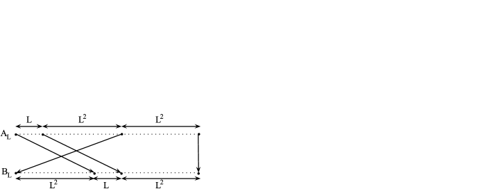
Figure 1: Monotonic rough isometry must have large constants.

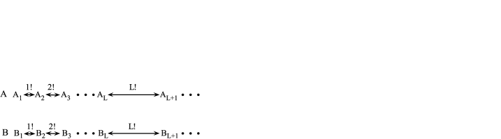
Figure 2: No monotonic rough isometry exists.

Although this example involves two finite sets of points and, of course, any two finite sets are increasing rough isometric for some constants, one may use this example to construct two infinite sets of points which are rough isometric, but not increasing rough isometric. Figure 2 shows two such sets $A$ and $B$ which are constructed by concatenating the previous $(A_{L},B_{L})$ example, but with a gap of size $L!$ in both $A$ and $B$ between $(A_{L},B_{L})$ and $(A_{L+1},B_{L+1})$. On the one hand, concatenating the rough isometries of Figure 1 gives a rough isometry with finite constants here, but, on the other hand, such a fast growing gap ensures that any rough isometry between $A$ and $B$ will have some large $L$ (depending on its constants) such that for all $j\geq L$, the points of $A_{j}$ will only be mapped to the points of $B_{j}$, thereby reducing to the example of Figure 1 within each such segment. In particular, the rough isometry cannot be monotonic.

In our context, it is then natural to ask the following question.

Main Open Question 3.

Given two independent Poisson processes $A,B$, does there exist a (weakly) increasing rough isometry between them a.s.?

As in Section 2, one can prove the following.

Proposition 3.1.

Given two independent Poisson processes $A,B\subseteq\mathbb{R}$ (possibly of different intensities) and constants $(M,D,R)$, the event that $A$ and $B$ are increasing rough isometric with constants $(M,D,R)$ is a zero-one event.

We also have the following equivalences.

Proposition 3.2.

The following are equivalent:

for some intensities $\alpha,\beta>0$, two independent Poisson processes, one with intensity $\alpha$ and the other with intensity $\beta$, are increasing rough isometric a.s.;

for any intensities $\alpha,\beta>0$, two independent Poisson processes, one with intensity $\alpha$ and the other with intensity $\beta$, are increasing rough isometric a.s.;

for some $0<p,q<1$, two independent Bernoulli percolations on $\mathbb{Z}$, one with parameter $p$ and the other with parameter $q$, are increasing rough isometric a.s.;

for any $0<p,q<1$, two independent Bernoulli percolations on $\mathbb{Z}$, one with parameter $p$ and the other with parameter $q$, are increasing rough isometric a.s.

The proofs of these statements are exactly the same as in Section 2, but with “rough isometry” replaced by “increasing rough isometry,” and are hence omitted. Again, due to these equivalences, we shall only consider Poisson processes of unit intensity and Bernoulli percolations with parameter $\frac{1}{2}$.

Analogously to Section 2, we can define a rooted increasing rough isometry between two rooted spaces $(X,a)$ and $(Y,b)$, where $X,Y\subseteq\mathbb{R}$, as a mapping $T\dvtx X\to Y$ which is an increasing rough isometry and has $T(a)=b$. For increasing rough isometries, it is much easier to pass from the question about percolations on $\mathbb{Z}$ to the question about percolations on $\mathbb{N}$, and from there to the finite version. This is due to the following obvious statement.

Proposition 3.3.

If $A,B\subseteq\mathbb{R}$ are increasing rough isometric by a mapping $T\dvtx A\to B$ with constants $(M,D,R)$, then, for any $x,y\in A$ with $x<y$, we have that $T$ restricted to $A\cap[x,y]$ is an increasing rough isometry from $A\cap[x,y]$ to $B\cap[T(x),T(y)]$ with constants $(M,D,R)$.

We emphasize once more that this statement is not true for general rough isometries, although, for increasing rough isometries, it is trivial to check that it holds (we omit the proof). From this, we easily deduce the following result.

Theorem 3.4.

The following are equivalent:

two independent Bernoulli percolations on $\mathbb{Z}$ are increasing rough isometric a.s.;

two independent rooted Bernoulli percolations $(A,0)$ and $(B,0)$ on $\mathbb{N}$ are rooted increasing rough isometric with positive probability;

there exists some $p>0$ and constants $(M,D,R)$ such that, given two independent rooted Bernoulli percolations $(A,0)$ and $(B,0)$ on $\mathbb{N}$, for any $n\geq 1$, $A(n)$ is a rooted increasing r.i. to some initial segment of $B$ with constants $(M,D,R)$ and with probability at least $p$.

Using Proposition 3.3, the equivalences $\mbox{(i)}\to\mbox{(ii)}$ and $\mbox{(ii)}\to\mbox{(iii)}$ are trivial to prove. The proofs of $\mbox{(ii)}\to\mbox{(i)}$ and $\mbox{(iii)}\to\mbox{(ii)}$ are the same as those given in Theorems 2.3 and 2.5, with “rough isometry” replaced by “increasing rough isometry.”

Of course, one can now formulate a quantitative version of our question, as follows.

Main Open Question 4.

Given two independent rooted Bernoulli percolations $(A,0)$ and $(B,0)$ on $\mathbb{N}$, for which functions $(M(n),D(n),R(n))$ does there exist an increasing rooted rough isometry $T$ with constants $(M(n),D(n),\break R(n))$ from $(A(n),0)$ to $(B(m),0)$ for some $m$ (a function of $A$, $B$ and $n$) with probability not tending to 0 with $n$?

As was mentioned earlier, Theorem 2.9 is still relevant in this context since the rough isometries we construct there are increasing rough isometries.

Until now, we have stated the common features of general rough isometries and increasing rough isometries. The next two subsections present some features which are unique to increasing rough isometries, revealing more of the interest in this concept. The first of these is a structure present in increasing rough isometries which we find quite interesting, although, unfortunately, we have not found a way to use it to our benefit in the sequel. The second of these is a slight variant on rooted increasing rough isometries which will be much easier for us to construct than general rough isometries; this variant is fundamental to our construction in Section 5.

3.1 Increasing rough isometries as finite distributive lattices

In this subsection, we shall show that, given constants $(M,D,R)$ and two finite subsets $A,B\subseteq\mathbb{N}\cup\{0\}$, both containing 0, the set of rooted increasing rough isometries from $A$ to $B$ with constants $(M,D,R)$ is either empty or a finite distributive lattice. This immediately implies a host of correlation inequalities (such as the FKG inequality), as discussed below. However, although we consider this to be a very interesting fact and a possibly useful structure, we should mention at the outset that we do not use this fact in our results and only include it here in the hope that it will prove useful in further work on the problem.

We start with (see, e.g., AS00 , Chapter 6) the following definition.

Definition 3.1.

A finite partially ordered set $L$ is called a finite distributive lattice if any two elements $x,y\in L$ have a unique minimal upper bound $x\vee y$ (called the join of $x$ and $y$) and a unique maximal lower bound $x\wedge y$ (called the meet of $x$ and $y$), such that, for any $x,y,z\in L$,

$$x\wedge(y\vee z)=(x\wedge y)\vee(x\wedge z).$$ (1)

Now, fix constants $(M,D,R)$ and finite subsets $A,B\subseteq\mathbb{N}\cup\{0\}$, both containing 0, which are rooted increasing r.i. with constants $(M,D,R)$. Let $L$ be the set of all such rooted increasing r.i. mappings from $A$ to $B$. For $T_{1},T_{2}\in L$, we write $T_{1}\preceq T_{2}$ if, for all $x\in A$, we have $T_{1}(x)\leq T_{2}(x)$. We also define $T_{1}\vee T_{2}$ as $(T_{1}\vee T_{2})\dvtx A\to B$, $(T_{1}\vee T_{2})(x):=\max(T_{1}(x),T_{2}(x))$ and, similarly, $(T_{1}\wedge T_{2})(x):=\min(T_{1}(x),T_{2}(x))$. It is clear that if $(T_{1}\vee T_{2})\in L$, then it is the unique minimal upper bound of $T_{1}$ and $T_{2}$ in $L$ and, similarly, that if $(T_{1}\wedge T_{2})\in L$, then it is their unique maximal lower bound. It is also clear that the distributive property (1) holds. Therefore, to show that $L$ is a finite distributive lattice, it remains to show the following.

Lemma 3.5.

For any $T_{1},T_{2}\in L$, we have $(T_{1}\vee T_{2}),(T_{1}\wedge T_{2})\in L$. Or, in words, the maximum and minimum of two rooted increasing r.i.’s with constants $(M,D,R)$ are also rooted increasing r.i.’s with constants $(M,D,R)$.

We remark that this lemma is not true for general rooted rough isometries as it is easy to see, by means of examples, that the monotonicity property is required. Proof of Lemma 3.5 We shall show this for $T_{1}\vee T_{2}$, the proof for $(T_{1}\wedge T_{2})$ being analogous (or even deducible from the $T_{1}\vee T_{2}$ case by considering the reversed mappings). Letting $T:=T_{1}\vee T_{2}$, it is clear that $T(0)=0$ and that $T$ is still (weakly) monotonic. We continue by verifying property (ii) in the definition of r.i. (see Figure 3). If we fix $b\in B$, then there exist $x,y\in A$ with $|T_{1}(x)-b|\leq R$ and $|T_{2}(y)-b|\leq R$ and we may assume, without loss of generality, that $x\leq y$. Of course, if $T(x)=T_{1}(x)$, then property (ii) holds, hence we assume that $T(x)=T_{2}(x)$. We obtain that $T_{1}(x)\leq T(x)=T_{2}(x)\leq T_{2}(y)$, from which $|T(x)-b|\leq R$ readily follows.

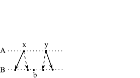
Figure 3: $T_{1}$: solid line; $T_{2}$: dashed line.

Fixing $x,y\in A$, $x<y$, it remains to verify property (i) in the definition of r.i. for $T$ and $x,y$ (see also Figure 3). If $T(x)=T_{i}(x)$ and $T(y)=T_{i}(y)$ for $i=1$ or $i=2$, then the properties clearly hold since they hold for $T_{i}$, hence we assume, without loss of generality, that $T(x)=T_{2}(x)>T_{1}(x)$ and $T(y)=T_{1}(y)>T_{2}(y)$, to obtain

$$\frac{1}{M}(y-x)-D\leq T_{2}(y)-T_{2}(x)<T(y)-T(x)<T_{1}(y)-T_{1}(x)\leq M(y-x)+D,$$

proving the lemma.

The usefulness of the finite distributive lattice structure in probability lies in the fact that it allows one to obtain correlation inequalities in many cases. Following AS00 , Chapter 6, we have the following definition and theorem.

Definition 3.2.

A probability measure $\mu$ on $L$ is called log-supermodular if, for all $T_{1},T_{2}\in L$,

$$\mu(T_{1})\mu(T_{2})\leq\mu(T_{1}\vee T_{2})\mu(T_{1}\wedge T_{2}).$$

Theorem 3.6 ((FKG inequality)).

If $\mu$ is log-supermodular and $f,g\dvtx L\to\mathbb{R}_{+}$ are increasing [in the sense that $f(T_{1})\leq f(T_{2})$ whenever $T_{1}\preceq T_{2}$], then

$$\mathbb{E}_{\mu}fg\leq(\mathbb{E}_{\mu}f)(\mathbb{E}_{\mu}g).$$

In our case, one may take, for example, $\mu$ to be the uniform measure on $L$, and, supposing $x,y\in A$, we may take $f(T_{1})=T_{1}(x)$ and $g(T_{1})=T_{1}(y)$. We immediately obtain that when sampling a rough isometry uniformly from $L$,the images of $x$ and $y$ are positively correlated. This example may not be so impressive since the result is intuitive, but, it is still not obvious how to prove this result directly (for arbitrary r.i. $A$ and $B$) and the significant point is that we obtained it here for free from the structure of $L$.

3.2 Markov rough isometries

In this subsection, we introduce a slightly different (but equivalent up to constants) definition of a rooted increasing rough isometry which will be much easier to work with in the sequel.

Definition 3.3.

Two subsets $A,B\subseteq\mathbb{N}\cup\{0\}$ both containing $0$ are Markov rough isometric if there exists a mapping $T\dvtx A\to B$ and constants $M,F,R\geq 0$ such that:

$T(0)=0$;

if $x,y\in A$ and $x\geq y$, then $T(x)\geq T(y)$;

for all adjacent $x,y\in A$ (i.e., with no point of $A$ between $x$ and $y$) with $T(x)\neq T(y)$, we have $\frac{1}{M}|x-y|\leq|T(x)-T(y)|\leq M|x-y|$;

for all $b\in T(A)$, we have $\max T^{-1}(b)-\min T^{-1}(b)\leq F$;

for any $b\in B$, there exists $x\in A$ such that $|T(x)-b|\leq R$.

The reason for the name “Markov rough isometry” is that all of the restrictions in the definition are, in some sense, local. To check that a given mapping $T$ is a valid Markov rough isometry, one scans its values on $A$ starting from $0$ and proceeding in increasing order. To check the properties, one needs to remember the value of $T$ on a point $x\in A$ only until one reaches a point $y>x$ with $T(y)>T(x)$ and, by property (iv), this must happen after checking at most $F$ points. Hence, there is a form of finite-memory property for Markov rough isometries, which accounts for the name. Still, although they may appear weaker at first, Markov rough isometries are equivalent to rooted increasing rough isometries as follows.

Lemma 3.7.

Fix two subsets $A,B\subseteq\mathbb{N}\cup\{0\}$, both containing $0$.

1. If $T\dvtx A\to B$ is a Markov rough isometry with constants $(M,F,R)$, then $T$ is a rooted increasing rough isometry with constants $(2F+M,\frac{1}{2},R)$.

2. If $T\dvtx A\to B$ is a rooted increasing rough isometry with constants $(M,D,R)$, then $T$ is a Markov rough isometry with constants $(MD+M+D,MD,R)$.

1. Let $T\dvtx A\to B$ be a Markov rough isometry with constants $(M,F,R)$ and define $(\widetilde{M},\widetilde{D},\widetilde{R}):=(2F+M,\frac{1}{2},R)$. To show that $T$ is a rooted increasing r.i. with constants $(\widetilde{M},\widetilde{D},\widetilde{R})$, only property (i) in the definition of rough isometry needs to be checked. If we let $x,y\in A$, $x<y$, and first suppose that $T(x)\neq T(y)$, then we can find some $k\geq 2$ and a sequence of points of $A$, $x\leq z^{1}_{r}<z^{2}_{l}\leq z^{2}_{r}<\cdots<z^{k-1}_{l}\leq z^{k-1}_{r}<z^{k}_{l}\leq y$, such that for each $i$, $z^{i}_{r}$ is adjacent in $A$ to $z^{i+1}_{l}$, $T(z^{i}_{r})\neq T(z^{i+1}_{l})$, $T(z^{i}_{l})=T(z^{i}_{r})$, $T(x)=T(z^{1}_{r})$ and $T(y)=T(z^{k}_{l})$ (Figure 4 shows an example with $k=5$). Then

   $$y-x = (y-z^{k}_{l})+(z^{k}_{l}-z^{k-1}_{r})+(z^{k-1}_{r}-z^{k-1}_{l})+\cdots+(z^{1}_{r}-x)$$

   $$\leq kF+M\bigl{(}T(z^{k}_{l})-z^{k-1}_{r}\bigr{)}+\cdots+M\bigl{(}T(z^{2}_{l})-T(z^{1}_{r})\bigr{)}$$

   $$= kF+M\bigl{(}T(y)-T(x)\bigr{)}$$

   and noting that $T(y)-T(x)\geq k-1$ [and, in particular, that $T(y)-T(x)\geq 1$], we obtain

   $$y-x \leq kF+M\bigl{(}T(y)-T(x)\bigr{)}\leq 2\bigl{(}T(y)-T(x)\bigr{)}F+M\bigl{(}T(y)-T(x)\bigr{)}$$

   $$= \widetilde{M}\bigl{(}T(y)-T(x)\bigr{)}.$$

   The lower bound follows more easily:

   $$y-x \geq (z^{k}_{l}-z^{k-1}_{r})+(z^{k-1}_{l}-z^{k-2}_{r})+\cdots+(z^{2}_{l}-z^{1}_{r})$$

   $$\geq \frac{1}{M}\bigl{(}T(z^{k}_{l}-z^{k-1}_{r})+\cdots+T(z^{2}_{l})-T(z^{1}_{r})\bigr{)}=\frac{1}{M}\bigl{(}T(y)-T(x)\bigr{)}.$$

   

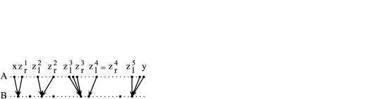
   Figure 4: An example for Lemma 3.7 with $k=5$.

   If we now suppose that $x,y\in A$, $x<y$, satisfy $T(x)=T(y)$, then $y-\break x\leq F$, hence

   $$0=T(y)-T(x)\geq\frac{1}{2F+M}(y-x)-\frac{1}{2}=\frac{1}{\widetilde{M}}(y-x)-\widetilde{D}$$

   as required.

2. Let $T\dvtx A\to B$ be a rooted increasing rough isometry with constants $(M,D,R)$ and define $(\widetilde{M},\widetilde{F},\widetilde{R})=(MD+M+D,MD,R)$. To show that $T$ is a Markov r.i. with constants $(\widetilde{M},\widetilde{D},\widetilde{R})$, only properties (iii) and (iv) in the definition of Markov rough isometry need to be checked. If we let $x,y\in A$ with $x$ adjacent to $y$ and $T(x)\neq T(y)$, then

   $$y-x\leq M\bigl{(}T(y)-T(x)+D\bigr{)}\leq(M+MD)\bigl{(}T(y)-T(x)\bigr{)}\leq\widetilde{M}\bigl{(}T(y)-T(x)\bigr{)}$$

   and

   $$T(y)-T(x)\leq M(y-x)+D\leq(M+D)(y-x)\leq\widetilde{M}(y-x).$$

   If we now suppose that $x,y\in A$ satisfy $T(x)=T(y)$, then we have

   $$0=T(y)-T(x)\geq\frac{1}{M}(y-x)-D,$$

   hence $y-x\leq MD=\widetilde{F}$, as required.

We conclude this subsection by remarking that some properties of rooted increasing rough isometries also hold for Markov rough isometries (without the need to change the constants). First, it is trivial to check the following (analogous to Proposition 3.3).

Proposition 3.8.

If $A,B\subseteq\mathbb{R}$ are Markov rough isometric by a mapping $T\dvtx A\to B$ with constants $(M,F,R)$, then, for any $x,y\in A$ with $x<y$, we have that $T$ restricted to $A\cap[x,y]$ is a Markov rough isometry from $A\cap[x,y]$ to $B\cap[T(x),T(y)]$ with constants $(M,F,R)$.

Second, we have the following proposition.

Proposition 3.9.

Given $A,B\subseteq\mathbb{N}\cup\{0\}$, both containing 0, which are Markov rough isometric with constants $(M,F,R)$, the set $L$ of all Markov rough isometries between them with constants $(M,F,R)$ is a finite distributive lattice (with the same operations as defined in Section 3.1).

The proof is very similar to the proof of Lemma 3.5 and is therefore omitted.

4 Proof of equivalence theorems

We start with the proof of Proposition 2.1. Proof of Proposition 2.1 We will use the well-known fact that a Poisson process on $\mathbb{R}$ with the shift operation on $\mathbb{R}$ is ergodic. We also note that the event $E$ that $A$ and $B$ are rough isometric with constants $(M,D,R)$ is measurable with respect to $A$ and $B$. Next, we note that for any fixed realization of $B$, the event $E_{B}$ that $A$ is rough isometric to $B$ with constants $(M,D,R)$ is translation invariant (with respect to translations of $A$), hence, by ergodicity, it has probability $0$ or $1$. Analogously, for any fixed realization of $A$, the event $E_{A}$ that $A$ is rough isometric to $B$ with constants $(M,D,R)$ is also translation invariant (with respect to translations of $B$) and hence has probability $0$ or $1$. It now follows from the independence of $A$ and $B$ that $E$ itself has probability $0$ or $1$.

We continue with the proof of Proposition 2.2. Proof of Proposition 2.2 $\mbox{(ii)}\to\mbox{(i)}$. This is trivial.

$\mbox{(i)}\to\mbox{(ii)}$. Suppose that claim (i) holds for some $\alpha,\beta>0$. Fix $\gamma>0$ and consider two Poisson processes $A$ and $C$, with intensities $\alpha$ and $\gamma$, respectively. Note that they can be coupled by first sampling $A$ and then letting the points of $C$ be $\{\frac{\alpha}{\gamma}x|x\in A\}$. Now, observe that under this coupling, $A$ and $C$ are r.i. with constants $(\frac{\alpha}{\gamma},0,0)$ under the trivial mapping $T\dvtx A\to C$ defined by $T(x):=\frac{\alpha}{\gamma}x$.

In the same way, if we fix some $\delta>0$, then we can couple two Poisson processes $B$ and $D$, with intensities $\beta$ and $\delta$, respectively, so that they are rough isometric a.s. Considering now two such independent Poisson processes $A$ and $B$, and the processes $C$ and $D$ which are coupled to them, we find that $C$ and $D$ are also independent and that they are rough isometric a.s. by transitivity of the rough isometry relation since $C$ and $A$ are rough isometric a.s. by our coupling, $A$ and $B$ are rough isometric a.s. using (i) and $B$ and $D$ are rough isometric a.s. by our coupling.

By means of similar transitivity arguments, to prove that (iii) and (iv) are equivalent to (i) and (ii), it is enough to establish that for any $\alpha>0$ and $0<p<1$, a Poisson process $A$ of intensity $\alpha$ and a Bernoulli percolation $\mathcaligr{A}$ with parameter $p$ can be coupled to be rough isometric a.s. We now show this. If we fix $\alpha$ and $p$ to have a coupling first sample $A$, then $\mathcaligr{A}$ will have a point at the integer $n$ if and only if $A$ has at least one point in the interval $[nc,(n+1)c)$, where $c=-\frac{\log(1-p)}{\alpha}$ is chosen so that this is indeed a coupling. Now, define a mapping $T\dvtx\mathcaligr{A}\to A$ by $T(n):=x_{n}$, where $x_{n}$ is some point of $A$ in the interval $[nc,(n+1)c)$, say the smallest one. It is easy to see that $T$ is a rough isometry with constants $(\max(c,\frac{1}{c}),c,c)$ since if $n,n+k\in\mathcaligr{A}$, then $(k-1)c\leq T(n+k)-T(n)\leq(k+1)c$.

4.1 Proof of Theorem 2.3

We first prove Lemma 2.4. Proof of Lemma 2.4 Let $A$ and $B$ be two independent Bernoulli percolations on $\mathbb{Z}$. First, by assumption, there exist constants $(M,D,R)$ such that $A$ and $B$ are rough isometric a.s. with constants $(M,D,R)$. Let $\Omega^{1}$ be this event.

Second, for $k,l,m\in\mathbb{Z}$ with $k<l<m$, let $\Omega^{2}_{k,l,m}$ be the event that $k,l,m\in A$, $l$ and $m$ are adjacent in $A$ (no point of $A$ lies between them) and $m-l\geq\frac{l-k}{M^{2}}-\frac{2D}{M}$. Noting that for fixed $k$, we have $\mathbb{P}(\Omega^{2}_{k,l,m})\leq 2^{-(m-l)}1_{(m-l)\geq c(l-k)-C}$ for some $C,c>0$, we get

$$\sum_{(m,l|m>l>k)}\mathbb{P}(\Omega^{2}_{k,l,m})\leq\sum_{(l|l>k)}2^{-c(l-k)+C+1}<\infty.$$

The Borel–Cantelli lemma then implies that with probability 1, only finitely many $\Omega^{2}_{k,l,m}$ occur for a fixed $k$.

Third, we condition on the events $\Omega^{1}$ and the event that for each $k$, only finitely many $\Omega^{2}_{k,l,m}$ occur. We fix two realizations $A$ and $B$, and let $T\dvtx A\to B$ be the r.i. between them. We will show (a deterministic claim) that there exists a cut point for $T$. To see this, fix $a\in A$ and let $b:=T(a)\in B$, noting that if there are only finitely many $u_{n}\in A$ with $u_{n}>a$ and $T(u_{n})<b$, then if we take $x$ to be the largest of these $u_{n}$, $x$ will satisfy ($\alpha$) in the definition of cut point. Analogously, if there were only finitely many $v_{n}\in A$ with $v_{n}>a$ and $T(v_{n})>b$, then ($\beta$) (in the definition of cut point) would be satisfied for some $x$. Hence, we assume, by way of contradiction, that there are infinitely many such $u_{n}$ and $v_{n}$. Since only finitely many $x\in A$ can be mapped to $b$, we must have infinitely many pairs $v,u\in A$, adjacent in $A$ with $a<v<u$, $T(v)>b$ and $T(u)<b$. Each such pair must satisfy

$$u-v\geq\frac{1}{M}\bigl{(}T(v)-T(u)-D\bigr{)}\geq\frac{1}{M}\bigl{(}T(v)-b-D\bigr{)}\geq\frac{1}{M}\biggl{(}\frac{1}{M}(v-a)-2D\biggr{)},$$

but this is a contradiction since only finitely many $\Omega^{2}_{a,l,m}$ occur. Proof of Theorem 2.3 $\mbox{(ii)}\to\mbox{(i)}$. Let $A$ and $B$ be two independent Bernoulli percolations on $\mathbb{Z}$. With probability $\frac{1}{4}$, they both contain $0$. Conditional on this event, let $(A^{+},0)$ be the rooted Bernoulli percolation on $\mathbb{N}$ obtained from $A$ by considering only the nonnegative integers. Define similarly the independent $(A^{-},0)$ obtained by considering the nonpositive integers, and the independent $(B^{+},0)$ and $(B^{-},0)$. By (ii), there exist constants $(M,D,R)$ such that, with positive probability, $(A^{+},0)$ is rooted r.i. to $(B^{+},0)$ and $(A^{-},0)$ is rooted r.i. to $(B^{-},0)$ with these constants. Denote these r.i. mappings by $T^{+}$ and $T^{-}$, respectively. Let the map $T\dvtx A\to B$ be the map whose restriction to $A^{+}$ is $T^{+}$ and whose restriction to $A^{-}$ is $T^{-}$. It is then easy to check directly from the definition that $T$ is a r.i. of $A$ to $B$ with constants $(M,2D,R)$. This shows that, with positive probability, $A$ and $B$ are r.i., but according to Propositions 2.1 and 2.2, $A$ and $B$ are r.i. with probability $0$ or $1$. Hence, $A$ and $B$ are rough isometric a.s.

$\mbox{(i)}\to\mbox{(ii)}$. Let $p$ be the probability that two independent rooted Bernoulli percolations on $\mathbb{N}$ are rooted r.i. We need to show that $p>0$. Let $A$ and $B$ be two independent Bernoulli percolations on $\mathbb{Z}$. For $n,m\in\mathbb{Z}$, let $A_{n}^{+}$ be all points of $A$ not smaller than $n$ and let $A_{n}^{-}$ be all points of $A$ not larger than $n$; similarly define $B_{m}^{+}$ and $B_{m}^{-}$. Let $E^{+}_{n,m}$ be the event that $n\in A$, $m\in B$ and there exists a rooted r.i. between $(A_{n}^{+},n)$ and $(B_{m}^{+},m)$; similarly define $E^{-}_{n,m}$ using $A_{n}^{+}$ and $B_{m}^{-}$. Note that $\mathbb{P}(E^{+}_{n,m})=\mathbb{P}(E^{-}_{n,m})=\frac{p}{4}$. Now, since by (i) and Lemma 2.4, with probability 1, there exists a r.i. $T\dvtx A\to B$ with a cut point $x\in A$, we get that $\mathbb{P}(\bigcup_{n,m}(E^{+}_{n,m}\cup E^{-}_{n,m}))=1$. This implies that $p>0$, proving the claim.

4.2 Proof of Theorem 2.5 and related lemmas

We start with the following proof. Proof of Lemma 2.6 Let $z\in A$ be the largest point such that $T(z)\leq T(x)$. Note that $z$ must be finite [since $T(0)=0$ and $A$ is infinite] and that $z\geq y>x$. First, note that for large enough $L$ (as a function of $M$ and $D$),

$$z-x\geq y-x\geq\frac{T(x)-T(y)-D}{M}\geq\frac{L-D}{M}\geq\frac{L}{2M}.$$ (2)

Second, let $w:=\operatorname{Succ}(z)$. Note that, by definition of $z$, we have $T(w)>T(x)\geq T(z)$, hence,

$$w-z \geq \frac{T(w)-T(z)-D}{M}>\frac{T(x)-T(z)-D}{M}$$

$$\geq \frac{1}{M}\biggl{(}\frac{z-x}{M}-2D\biggr{)}$$

$$= \frac{z-x}{M^{2}}-\frac{2D}{M}$$

and, by combining this inequality with (2), we see that if $L$ is large enough (as a function of $M$ and $D$), then $w-z\geq\frac{z-x}{2M^{2}}$, as required.

We next show the following. Proof of Lemma 2.7 For any fixed $z\in\mathbb{N}$, $\mathbb{P}(\operatorname{Gap}(z)\geq k)\leq 2^{-(k-1)}$ (with equality if $k$ is a positive integer). Hence, by a union bound,

$$\mathbb{P}(E^{w}_{L,M}) \leq \biggl{(}\frac{L}{2M}+1\biggr{)}2^{-({L}/({4M^{3}})-1)}+\sum_{i=\lceil{L}/({2M})\rceil}^{\infty}2^{-({i-1})/({2M^{2}})}$$

$$\leq C\biggl{(}\frac{L}{M}+1\biggr{)}e^{-c{L}/({M^{3}})}.$$

We continue with the following proof. Proof of Lemma 2.8 Letting $x_{i}\in A$ be the $i$th point of $A$ and $a_{i}$ be the $i$th point of $B$, we choose $m$ so that $a_{m}=\max_{1\leq i\leq n}T(x_{i})$ [i.e., the minimal $m$ such that $T(A(n))\subseteq B(m)]$. First, for any $x,y\in A(n)$, we have

$$\frac{1}{M}|x-y|-D\leq|T(y)-T(x)|\leq M|x-y|+D,$$

by the properties of $T$. Second, to reach a contradiction, assume that for some $b\in B(m)$ and for all $x\in A(n)$, $|T(x)-b|>L$. Since $T$ is a rooted r.i. with constants $(M,D,R)$, there must exist some $y\in A$, $y>x_{n}$ with $|T(y)-b|\leq R$; furthermore, by the minimality of $m$, there must exist some $x\in A(n)$ with $T(x)>b+L$, hence $x\leq x_{n}<y$ and $T(x)-T(y)\geq L-R$. By Lemma 2.6, there exists some $z\in A$, $z\geq y$ and $z-x\geq\frac{L-R}{2M}$ such that $\operatorname{Gap}(z)\geq\frac{z-x}{2M^{2}}$. But, then, in particular, $z>x_{n}$ and $\operatorname{Gap}(z)\geq\max(\frac{L-R}{4M^{3}},\frac{z-x_{n}}{2M^{2}})$, which contradicts the fact that $E^{x_{n}}_{L-R,M}$ does not hold for $A$.

Finally, we have the following proof.

Proof of Theorem 2.5 $\mbox{(i)}\to\mbox{(ii)}$. Let $(A,0)$ and $(B,0)$ be two independent rooted Bernoulli percolations on $\mathbb{N}$ and let $E$ be the event that they are rooted r.i. with constants $(M,D,R)$. Suppose that $\mathbb{P}(E)\geq r$ for some $r>0$. On the event $E$, let $T\dvtx A\to B$ be such a rooted r.i. Fix $n\geq 1$, let $x_{n}\in A$ be the $n$th point of $A$, fix $L>R$ and let $E^{x_{n}}_{L-R,M}$ be the event from Lemma 2.7. Note that since $x_{n}$ is a stopping time for the percolation $A$ (i.e., $\{x_{n}>k\}$ only depends on whether $i\in A$ for $0\leq i\leq k$) and since $E^{x}_{L,M}$ only depends on the future of $x$ (i.e., on the events $\{i\in A\}_{i>x}$), we have, by Lemma 2.7, that $\mathbb{P}(E^{x_{n}}_{L-R,M})\leq C(\frac{L-R}{M}+1)e^{-c({L-R})/({M^{3}})}$ for some absolute constants $C,c>0$. Hence, for each fixed $0<p<r$, we can choose $L$ sufficiently large (uniformly in $n$) so that $\mathbb{P}(E\cap(E^{x_{n}}_{L-R,M})^{c})\geq p$; we fix such a pair of $p$ and $L$. We are now done since, on the event $E\cap(E^{x_{n}}_{L-R,M})^{c}$, Lemma 2.8 gives that $T$ restricted to $A(n)$ is a rooted r.i. of $A(n)$ to some initial segment of $B$ with constants $(M,D,L)$.

$\mbox{(ii)}\to\mbox{(i)}$. Let $E_{n}$ be the event that $A(n)$ is rooted r.i. to some initial segment of $B$ with constants $(M,D,R)$, so that by assumption that $\mathbb{P}(E_{n})\geq p>0$ for all $n$. Let $E:=\limsup E_{n}$, so that, by Fatou’s lemma, $\mathbb{P}(E)\geq\limsup\mathbb{P}(E_{n})\geq p$. Let $(A,B)\in E$, that is, $A$ and $B$ are two realizations of rooted Bernoulli percolation on $\mathbb{N}$ such that, for an infinite sequence $n_{k}\to\infty$ (depending on $A$ and $B$), there exists a rooted r.i. $T_{n_{k}}$ from $A(n_{k})$ to some initial segment of $B$ with constants $(M,D,R)$. We now deduce that $A$ and $B$ are themselves rooted r.i. with constants $(M,D,R)$. Let $x_{i}$ be the $i$th point of $A$. To define $T\dvtx A\to B$, we need to pick $a_{i}\in B$ such that $T(x_{i}):=a_{i}$; we do this by induction. Since $x_{1}=0$, we also choose $a_{1}:=0$. Assume that we have already chosen $\{a_{i}\}_{i=1}^{N-1}$ for some $N\geq 2$ in such a way that there exists an infinite sequence $n^{j}:=n_{k_{j}}$ such that $T_{n^{j}}$ agrees with $T$ on $\{x_{i}\}_{i=1}^{N-1}$. To choose $a_{N}$, we note that $\{T_{n^{j}}(x_{N})\}_{j}$ is a finite set since, for example, for each $j$, $\frac{x_{N}}{M}-D\leq T_{n^{j}}(x_{N})\leq Mx_{N}+D$. Hence, we can choose $a_{N}$ in such a way that it agrees with an infinite subsequence of $\{T_{n^{j}}\}_{j}$. In this way, we obtain $T$.

To see that $T$ is a rooted r.i. with constants $(M,D,R)$, we note that for each $x,y\in A$, by our construction, there exists some $k$ such that $T_{n_{k}}$ agrees with $T$ on $x$ and $y$. Hence, $\frac{|x-y|}{M}-D\leq|T(x)-T(y)|\leq M|x-y|+D$. Next, we fix $b\in B$, choose $N$ sufficiently large that $x_{N}\geq M(b+R+D)$ and choose $k$ so that $T_{n_{k}}$ agrees with $T$ on $\{x_{i}\}_{i=1}^{N}$. Since $T_{n_{k}}$ is a rooted r.i., there exists $x\in A$ such that $|T(x)-b|\leq R$. We cannot have $x>X_{N}$ since, otherwise, $|T(x)|\geq\frac{x}{M}-D>\frac{x_{N}}{M}-D\geq b+R$. Hence, $x\leq x_{N}$ and so $|T(x)-b|\leq R$, as required. This completes the proof of the theorem.

5 The main construction

In this section, we shall prove Theorem 2.9. Let us recall the setting. We are given two independent rooted Bernoulli percolations $(A,0)$ and $(B,0)$ on $\mathbb{N}$. We will show that, for any large enough $n$ (independent of $A$ and $B$), there exists a Markov rough isometry from $A(n)$ to some initial segment of $B$ with constants $(10\sqrt{\log_{2}n},10\sqrt{\log_{2}n},10\sqrt{\log_{2}n})$ and with probability $1-2^{-8\sqrt{\log_{2}n}}$. As explained before, existence of a Markov rough isometry is a stronger statement than existence of a general rough isometry since Markov rough isometries are monotone and, by Lemma 3.7, the same mapping will also be a rooted increasing rough isometry with constants $(30\sqrt{\log_{2}n},\frac{1}{2},10\sqrt{\log_{2}n})$. The reason we construct a Markov rough isometry rather than an increasing rooted rough isometry is that we will frequently rely on the fact that one can check the validity of a Markov rough isometry by simply looking at local configurations (as explained in Section 3.2).

We fix $n$ very large. It would be convenient for us to assume that $M,F$ and $R$ are integers, hence we choose $0.99<\alpha<1$ (depending on $n$) so that $\alpha\sqrt{\log_{2}n}$ is an integer. We then let $M=F=R:=10\alpha\sqrt{\log_{2}n}$. We also introduce a new parameter, $K:=2^{\alpha\sqrt{\log_{2}n}}=(2^{M})^{{1}/{10}}$, whose use will be made clear in the sequel.

Given a sorted sequence $U:=(0,x_{1},x_{2},\ldots,x_{L})\subseteq\mathbb{N}\cup\{0\}$ (where we allow $L$ to be infinite), we define some notation. For a point $t\in U$, let $s^{U}(t)$ or, equivalently, $s_{1}^{U}(t)$ be its successor point in $U$; similarly, let $s_{k}^{U}(t)$ be its $k$th successor point in $U$ and define $s_{0}^{U}(t):=t$. We call the quantity $g^{U}(t):=s^{U}(t)-t$ the gap at $t$. When the set $U$ is clear from the context, we sometimes omit the superscript and simply write $s_{k}(t)$ and $g(t)$.

We will sometimes refer to $U$ equivalently by its gap sequence $\{G^{U}(i)\}_{i=1}^{L}$, defined by $G^{U}(i):=x_{i}-x_{i-1}$.

Let $A$ and $B$ be two independent rooted Bernoulli percolations $(A,0)$ and $(B,0)$ on $\mathbb{N}$. Note that for $A$ and $B$, the sequences $G^{A}$ and $G^{B}$ are simply i.i.d. $\operatorname{Geom}(\frac{1}{2})$ random variables.

We shall call a gap short if it less than or equal to $M$, otherwise we call it long.

5.1 Partitioning into blocks

The first thing we will do is to partition $A$ and $B$ into blocks (which overlap at their end points). Let us first describe this partition informally and then give a rigorous definition. Each block will consist of two parts, a “blue” initial segment followed by a “red” segment. A blue segment is a segment of the percolation points containing only short gaps (of length $\leq M$). A red segment is a segment of the percolation points starting with a long gap (of length $>M$) and ending just before $K$ short gaps (see Figure 5).

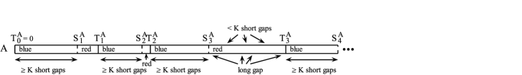
Figure 5: A sample of the first three blocks followed by the blue segment of the fourth block. The third red segment has long and short gaps indicated.

More formally, to define blocks in $A$, we define a sequence of times inductively, $T_{0}^{A}:=0$, and, for each $k\geq 1$,

$$S_{k}^{A} := \min\{t\in A|t>T^{A}_{k-1},g(t)>M\},$$

$$T_{k}^{A} := \min\{t\in A|t>S_{k}^{A},g(s_{i}(t))\leq M\mbox{ for all $0\leq i\leq K-1$}\}.$$

For each $k\geq 1$, $S_{k}^{A}$ is the first point in $A$ after $T_{k-1}^{A}$ and immediately preceding a gap longer than $M$, and $T_{k}^{A}$ is the first point in $A$ after $S_{k}^{A}$ which precedes $K$ short gaps.

The points of $A$ in the segment $[T_{k-1}^{A},T_{k}^{A}]$ constitute the $k$th block of $A$. In each block, the blue segment consists of the points in $[T_{k-1}^{A},S_{k}^{A}]$. By definition (except possibly for the first block), the blue segment has at least $K$ short gaps (and no long gaps). It is followed by a red segment, consisting of the points in $[S_{k}^{A},T_{k}^{A}]$, which starts with a long gap and continues until the starting point of a run of $K$ short gaps (not including that run). Note that the red segment may contain many long gaps or as few as one. Also, it must start with a long gap and end immediately after a long gap. The first block is different from the rest since it may have less than $K$ gaps in its blue segment. However, letting

$$E_{0}^{A}:=\{\mbox{$A$ starts with at least $K$ short gaps}\},$$ (4)

we have $\mathbb{P}(E_{0}^{A})=(1-\frac{1}{2^{M}})^{K}\geq 1-\frac{K}{2^{M}}=1-2^{-9\alpha\sqrt{\log_{2}n}}$. We emphasize that, conditioned on $E_{0}^{A}$, the distribution of blocks after subtracting their starting points (or, equivalently, when looking at their gap sequences) is i.i.d. and we shall refer to that common distribution as $\mathcaligr{L}^{\mathrm{block}}$, or, in words, the distribution of a rooted block.

We partition $B$ in the same way, into blocks analogously defining $T_{k}^{B}$, $S_{k}^{B}$ and $E_{0}^{B}$.

It will be useful to define the distributions of blocks and of blue and red segments precisely, which we now proceed to do.

Definition 5.1.

We say that $X\sim\operatorname{Geom}_{\leq M}(\frac{1}{2})$ if $X$ is distributed like a $\operatorname{Geom}(\frac{1}{2})$ random variable conditioned to be less than or equal to $M$. We say that $Y\sim\operatorname{Geom}_{>M}(\frac{1}{2})$ if $Y$ is distributed like a $\operatorname{Geom}(\frac{1}{2})$ random variable conditioned to be larger than $M$ or, in other words, as $M+\operatorname{Geom}(\frac{1}{2})$.

The following observation will be useful in the sequel. It is also true in much greater generality.

Lemma 5.1.

The $\operatorname{Geom}_{\leq M}(\frac{1}{2})$ distribution is stochastically dominated by the $\operatorname{Geom}(\frac{1}{2})$ distribution.

Define a coupling of $(X,Y)$ with $X\sim\operatorname{Geom}_{\leq M}(\frac{1}{2})$ and $Y\sim\operatorname{Geom}(\frac{1}{2})$ using the following algorithm: take an infinite sequence $(Z_{i})_{i=1}^{\infty}$ of i.i.d. $\operatorname{Geom}(\frac{1}{2})$ random variables, and let $Y=Z_{1}$ and $X=Z_{i}$, with $i$ the minimal index for which $Z_{i}\leq M$. It is then clear that $X\leq Y$ a.s.

Definition 5.2.

For a given integer $L>0$, say that $U:=(0,x_{1},x_{2},\ldots,\break x_{L})\subseteq\mathbb{N}\cup\{0\}$ is distributed $\mathcaligr{L}_{L}^{\mathrm{blue}}$, or in words, distributed as a rooted blue segment of length $L$ if $(x_{i}-x_{i-1})_{i=1}^{L}$ are i.i.d. $\operatorname{Geom}_{\leq M}(\frac{1}{2})$ (where $x_{0}:=0$).

Lemma 5.2.

Let $B=(0,x_{1},\ldots,x_{P},x_{P+1},\ldots,x_{Q})$ be a rooted block, with $U:=(0,x_{1},\ldots,x_{P})$ being its blue segment and $(x_{P},x_{P+1},\ldots,x_{Q})$ being its red segment. Also, let $V:=(0,x_{P+1}-x_{P},\ldots,x_{Q}-x_{P})=(0,y_{1},\ldots,y_{Q-P})$ be the red segment minus its starting point. Then:

1. $U$ and $V$ are independent;

2. $U$ is distributed $\mathcaligr{L}_{P}^{\mathrm{blue}}$, where $P$ is a random variable distributed $\operatorname{Geom}(\frac{1}{2^{M}})-1$, conditioned to be at least $K$ [or, in other words, $P\sim K-1+\operatorname{Geom}(\frac{1}{2^{M}})$], independently of the lengths of the gaps in the block;

3. the distribution of $V$ is characterized by:

   1. [(a)]

   2. $y_{1}\sim\operatorname{Geom}_{>M}(\frac{1}{2})$, independently of the other gaps;

   3. $y_{2},\ldots,y_{Q-P}$ are the concatenation of $N\sim\operatorname{Geom}((1-\frac{1}{2^{M}})^{K})-1$ subsequences which are i.i.d., given $N$. Each such subsequence starts with $Z$ gaps, each having distribution $\operatorname{Geom}_{\leq M}(\frac{1}{2})$ independently of each other and where $Z$ is distributed $\operatorname{Geom}(\frac{1}{2^{M}})-1$, conditioned to be less than $K$. The subsequence then continues with one last gap distributed $\operatorname{Geom}_{>M}(\frac{1}{2})$ independently of the other gaps.

The red segment begins at the first long gap of a block. It is clear that knowing the lengths of all of the gaps previous to this gap does not provide any additional information on the length of this or the following gaps.

The first, say, blue segment of $A$ contains all of the gaps up to the first long gap from the beginning of $A$. The length of this run of short gaps is $\operatorname{Geom}(\frac{1}{2^{M}})-1$ and it is independent of the lengths of the short gaps in it. Hence, conditioned that this run of short gaps contains at least $K$ gaps, we obtain the characterization given in the lemma.

The first, say, red segment of $A$ is defined to start where the first run of short gaps of $A$ ends and to continue until just before a run of at least $K$ short gaps. Hence, it can be described in the following way. First, since it ends a run of short gaps, it has to start with a long gap. Since the gaps in $A$ are i.i.d. and all we know about this gap is that it is long, its size will be independent of the size of all other gaps [but distributed $\operatorname{Geom}_{>M}(\frac{1}{2})]$. We then test to see if the following $K$ gaps are all short. If they are, then we end the red segment, otherwise we include the run of short gaps coming afterward and the long gap following it in the red segment. We now continue in the same manner with another independent trial to see if the next $K$ gaps are all short. If so, we end, otherwise we include them and the long gap at their end in the red segment. These independent trials continue until we finally find a run of at least $K$ short gaps. Hence, the number of trials is geometric (but we subtract one since once we succeed, we do not concatenate anything to the red segment) and its success parameter is $(1-\frac{1}{2^{M}})^{K}$, which is the probability of seeing $K$ short gaps in a row. When a trial fails, it means that the number of short gaps after it is less than $K$. Since, a priori, the number of short gaps is $\operatorname{Geom}(\frac{1}{2^{M}})-1$, we have that $Z$, the number of short gaps following a failed trial, is $\operatorname{Geom}(\frac{1}{2^{M}})-1$, conditioned to be less than $K$. Finally, the lengths of the short gaps themselves are unaffected by the number of short gaps in a run, hence they are all $\operatorname{Geom}_{\leq M}(\frac{1}{2})$, independently of everything else. Similarly, the length of the long gap which ends a run of short gaps is $\operatorname{Geom}_{>M}(\frac{1}{2})$, independently of everything else.

Definition 5.3.

We say that a vector having the distribution of the vector $V$ of the previous lemma is distributed $\mathcaligr{L}^{\mathrm{red}}$ or, in words, distributed as a rooted red segment.

5.2 Properties of blocks

In this subsection, we will prove some basic properties of rooted blue and red segments which will be useful for our construction in the sequel. We start with two properties of red segments.

Lemma 5.3.

Let $V\sim\mathcaligr{L}^{\mathrm{red}}$, $X$ be the number of long gaps in $V$ and $\{b_{i}\}_{i=1}^{X}$ be their lengths. There then exist $\beta,\gamma>0$ such that

$$\mathbb{P}\biggl{(}X>\frac{1}{8}\sqrt{\log_{2}n}\biggr{)} = o\biggl{(}\frac{1}{n^{1+\beta}}\biggr{)},$$

$$\mathbb{P}\Biggl{(}\sum_{i=1}^{X}b_{i}\geq 3\log_{2}n\Biggr{)} = o\biggl{(}\frac{1}{n^{1+\gamma}}\biggr{)}.$$

By Lemma 5.2, we know that $X\sim\operatorname{Geom}((1-\frac{1}{2^{M}})^{K})$. Hence,

$$\mathbb{P}\biggl{(}X>\frac{1}{8}\sqrt{\log_{2}n}\biggr{)} = \biggl{[}1-\biggl{(}1-\frac{1}{2^{M}}\biggr{)}^{K}\biggr{]}^{{1}/{8}\sqrt{\log_{2}n}}\leq\biggl{(}\frac{K}{2^{M}}\biggr{)}^{{1}/{8}\sqrt{\log_{2}n}}$$

$$= 2^{-{9}/{8}\alpha\log_{2}n}=o\biggl{(}\frac{1}{n^{1+\beta}}\biggr{)}$$

for some $\beta>0$, proving the first claim. Now, conditioned on $X$, the $\{b_{i}\}_{i=1}^{X}$ are i.i.d. with distribution $\operatorname{Geom}_{>M}(\frac{1}{2})$, that is, with distribution $M+\operatorname{Geom}(\frac{1}{2})$. Hence,

$$\mathbb{P}\Biggl{(}\sum_{i=1}^{X}b_{i}\geq 3\log_{2}n|X\Biggr{)} = \sum_{s\geq 3\log_{2}n}\mathop{\mathop{\sum}_{b_{1}+\cdots+b_{X}=s}}_{b_{i}>M}2^{-\sum_{i=1}^{X}(b_{i}-M)}$$

$$= 2^{MX}\sum_{s\geq 3\log_{2}n}2^{-s}\#\{b_{1}+\cdots+b_{X}=s|b_{i}>M\}$$

$$\leq 2^{10\alpha\sqrt{\log_{2}n}X}\sum_{s\geq 3\log_{2}n}2^{-s}s^{X},$$

so, denoting $E:=\{X\leq\frac{1}{8}\sqrt{\log_{2}n}\}$, we have, for large enough $n$ and some $C>0$,

$$\mathbb{P}\Biggl{(}\Biggl{\{}\sum_{i=1}^{X}b_{i}\geq 3\log_{2}n\Biggr{\}}\cap E\Biggr{)} \leq 2^{{10}/{8}\alpha\log_{2}n}\sum_{s\geq 3\log_{2}n}2^{-s}s^{{1}/{8}\sqrt{\log_{2}n}}$$

$$\leq 2^{{5}/{4}\alpha\log_{2}n}\sum_{s\geq 3\log_{2}n}2^{-s}s^{{1}/{8}\sqrt{{s}/{3}}}$$

$$\leq 2^{{5}/{4}\alpha\log_{2}n}\sum_{s\geq 3\log_{2}n}2^{-{4}/{5}s}$$

$$\leq C2^{{5}/{4}\alpha\log_{2}n-{12}/{5}\log_{2}n}=o\biggl{(}\frac{1}{n^{1+\widetilde{\gamma}}}\biggr{)}$$

for some $\widetilde{\gamma}>0$. Hence, by (5.2), we have $\mathbb{P}(\sum_{i=1}^{X}b_{i}\geq 3\log_{2}n)\leq o(\frac{1}{n^{1+\beta}})+o(\frac{1}{n^{1+\widetilde{\gamma}}})$, proving the second claim.

We continue with three properties of blue segments. We start with the following, simple, lemma.

Lemma 5.4.

For a given integer $L>0$ and $U:=(0,x_{1},x_{2},\ldots,x_{L})\sim\mathcaligr{L}_{L}^{\mathrm{blue}}$, if $0\leq T\leq L$ is a stopping time in the sense that the event $\{T\leq k\}$ depends only on $\{x_{i}\}_{i=1}^{k}$, then, conditioned on $T$, on the event $\{T<L\}$, the partial rooted segment $V:=(0,x_{T+1}-x_{T},\ldots,x_{L}-x_{T})$ is distributed $\mathcaligr{L}_{L-T}^{\mathrm{blue}}$.

Consider the gap sequence $G^{U}=(x_{1},x_{2}-x_{1},\ldots,x_{L}-x_{L-1})$. By definition, its elements are i.i.d. $\operatorname{Geom}_{\leq M}(\frac{1}{2})$. If we let $A_{k}:=\{T=k\}$ for $k<L$ and $B$ be an event that depends only on $(x_{k+1}-x_{k},\ldots,x_{L}-x_{k})$, then, since $A_{k}$ is determined by $(x_{1},\ldots,x_{k})$ and these are, in turn, determined by $(x_{1},x_{2}-x_{1},x_{k}-x_{k-1})$, we have that $A_{k}$ and $B$ are independent. Hence, conditioned on $A_{k}$, the probability of $B$ remains the same, implying that $(x_{k+1}-x_{k},\ldots,x_{L}-x_{k})$ are still i.i.d. $\operatorname{Geom}_{\leq M}(\frac{1}{2})$, proving the claim.

Lemma 5.5.

Fix integers $L,Z>0$ and let $U:=(0,x_{1},\ldots,x_{L})\sim\mathcaligr{L}_{L}^{\mathrm{blue}}$. Divide the points of $U$ into subsegments according to the following algorithm: the first subsegment consists of $(0,x_{1},x_{2},\ldots,x_{l_{1}})$ with $l_{1}$ maximal such that $x_{l_{1}}\leq Z$; by induction for $i\geq 2$, the $i$th subsegment consists of $(x_{l_{i-1}+1},\ldots,x_{l_{i}})$ with $l_{i}$ maximal such that $x_{l_{i}}-x_{l_{i-1}+1}\leq Z$. Let $Y$ be the number of subsegments required to cover all $L$ points. We claim that

$$\mathbb{P}\biggl{(}Y>\frac{3L}{Z}\biggr{)}\leq e^{-cL}$$

for some $c>0$.

First, note that the event $Y>m$ is contained in the event $x_{L}>mZ$. Hence, $\mathbb{P}(Y>\frac{3L}{Z})\leq\mathbb{P}(\sum_{i=1}^{L}G_{i}>3L)$, where the $G_{i}$ are i.i.d. $\operatorname{Geom}_{\leq M}(\frac{1}{2})$ random variables. Since a $\operatorname{Geom}_{\leq M}(\frac{1}{2})$ random variable is stochastically dominated by a $\operatorname{Geom}(\frac{1}{2})$ random variable, by Lemma 5.1, we get, by standard large deviation estimates, that $\mathbb{P}(\sum_{i=1}^{L}G_{i}>3L)\leq e^{-cL}$ for some $c>0$, as claimed.

The following lemma is a major ingredient in our rough isometry construction.

Lemma 5.6.

Let $(G_{i})_{i=1}^{\infty}$ be i.i.d. $\operatorname{Geom}_{\leq M}(\frac{1}{2})$ random variables, termed gaps. Let $m>0$, $M>a_{1},\ldots,a_{m}>0$ and $d_{1},\ldots,d_{m-1}\geq 0$ be given integers. We consider the $\{a_{i}\}$ as representing minimal required gap lengths and the $\{d_{i}\}$ as representing inter-gap distances. Say that a position $l$ is valid if $G_{l}\geq a_{1}$, $G_{l+d_{1}+1}\geq a_{2}$, $G_{l+d_{1}+1+d_{2}+1}\geq a_{3},\ldots,G_{l+m-1+\sum_{i=1}^{m-1}d_{i}}\geq a_{m}$. If we let $Z$ be the minimal valid position, then, for any $a>0$ and $s:=\sum_{i=1}^{m}a_{i}$,

$$\mathbb{P}(Z>\lceil a2^{s}\rceil)\leq e^{-{a}/{m^{2}}}.$$

Let $I_{l}$ be the event that $l$ is a valid position. Then

$$\mathbb{P}(I_{l})=\prod_{i=1}^{m}\biggl{(}\frac{1}{2^{a_{i}-1}}-\frac{1}{2^{M}}\biggr{)}\bigg{/}\biggl{(}1-\frac{1}{2^{M}}\biggr{)}\geq\prod_{i=1}^{m}\frac{1}{2^{a_{i}}}=\frac{1}{2^{s}}.$$

For a given position $l$, let us denote by $C_{l}:=(l,l+d_{1}+1,\ldots,l+m-1+\sum_{i=1}^{m-1}d_{i})$ the comb at position $l$ and say that two positions $l,k$ overlap if their combs intersect, that is, if $C_{l}\cap C_{k}\neq\varnothing$ (see Figure 6). Note that if $F\subseteq\mathbb{N}$ is a subset of positions, no two of which overlap, then $\{I_{l}\}_{l\in F}$ are independent.

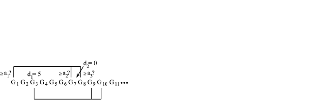
Figure 6: A comb at two nonoverlapping positions.

Fixing an integer $N>0$, to bound $\mathbb{P}(Z>N)$, we wish to choose a large collection of positions $F\subseteq\{1,\ldots,N\}$, no two of which overlap. We note that a given comb $C_{l}$ may only intersect at most $m(m-1)$ other combs $C_{k}$ since each overlapping position $k$ uniquely determines a pair of coordinates $1\leq i,j\leq m$, $i\neq j$, such that the $i$th coordinate of $C_{l}$ is equal to the $j$th coordinate of $C_{k}$ by, say, the smallest element of $C_{l}\cap C_{k}$. Hence, we can find such a collection $F$ with, say, $|F|\geq\lceil\frac{N}{m^{2}}\rceil$, by means of a greedy algorithm. Thus, we obtain the bound

$$\mathbb{P}(Z>N) \leq \mathbb{P}\biggl{(}\bigcap_{l\in F}I_{l}^{c}\biggr{)}=\prod_{l\in F}\bigl{(}1-\mathbb{P}(I_{l})\bigr{)}$$

$$\leq \biggl{(}1-\frac{1}{2^{s}}\biggr{)}^{\lceil{N}/{m^{2}}\rceil}\leq e^{-2^{-s}\lceil{N}/{m^{2}}\rceil}$$

and the claim follows by taking $N:=\lceil a2^{s}\rceil$.

Remark 5.1.

We point out that in the notation of the previous lemma, the position $Z+m-1+\sum_{i=1}^{m-1}d_{i}$ is a stopping time for the process $\{G_{i}\}_{i=1}^{\infty}$.

5.3 The construction

A major part of the construction of the rough isometry between $A$ and $B$ will be constructing a rough isometry between a block of $A$ and the beginning of a blue segment of $B$ or, alternatively, constructing a rough isometry between the beginning of a blue segment of $A$ and a block of $B$. The following theorem gives conditions under which this is possible with high probability.

Theorem 5.7.

Fix integers $L_{1},L_{2}$ satisfying $L_{2}\geq\max(K,L_{1})$ and $L_{1}\geq\frac{K}{2}$. Let $U^{1}:=(0,x^{1}_{1},\ldots,x^{1}_{L_{1}})\sim\mathcaligr{L}_{L_{1}}^{\mathrm{blue}}$, $U^{2}:=(0,x^{2}_{1},\ldots,x^{2}_{L_{2}})\sim\mathcaligr{L}_{L_{2}}^{\mathrm{blue}}$ and $V\dvtx(0,y_{1},\break\ldots,y_{N})\sim\mathcaligr{L}^{\mathrm{red}}$, where $N$ is random, with $U^{1},U^{2},V$ independent. Construct the segment $W:=(0,x^{1}_{1},\ldots,x^{1}_{L_{1}},x^{1}_{L_{1}}+y_{1},\ldots,x^{1}_{L_{1}}+y_{N})$ by concatenating $U^{1}$ and $V$. There then exists a random integer $1\leq S\leq L_{2}$ which is a stopping time for $U^{2}$ conditioned on $W$. That is, the event $\{S\leq l\}$ is measurable with respect to $W$ and $\{x_{i}^{2}\}_{i=1}^{l}$, satisfying the conditions that if $E=\{S\leq\max(\frac{K}{2},\frac{L_{1}}{\sqrt{\log_{2}n}})\}$, then:

$\mathbb{P}(E)=1-o(\frac{1}{n^{1+\delta}})$ for some $\delta>0$;

on the event $E$, there exists a Markov rough isometry $T_{1}$ from $W$ to $U^{2}\cap[0,x_{S}^{2}]$ with constants $(M,F,R)$ such that the last point of $W$ is mapped to $x_{S}^{2}$ and it is the only point mapped to $x_{S}^{2}$;

on the event $E$, there exists a Markov rough isometry $T_{2}$ from $U^{2}\cap[0,x_{S}^{2}]$ to $W$ with constants $(M,F,R)$ such that $x_{S}^{2}$ is mapped to the last point of $W$ and it is the only point mapped to the last point of $W$.

Let us show how to prove Theorem 2.9 using Theorem 5.7. We first require the following definition.

Definition 5.4.

For a given integer $L\geq 0$, a sorted infinite sequence $U:=(x_{1},x_{2},x_{3},\ldots)\subseteq\mathbb{N}\cup\{0\}$ is said to be distributed as a Bernoulli percolation with $L$ initial short gaps if the rooted sequence $V:=(0,x_{2}-x_{1},x_{3}-x_{1},\ldots)$ is distributed as a rooted Bernoulli percolation on $\mathbb{N}$ conditioned to have its first $L$ gaps short and its next gap long.

The proof is by induction: for each stage $0\leq j\leq n$, we shall have an event $E_{j}$ denoting whether or not the $j$th stage was successful, with $\mathbb{P}(E_{j}|\{E_{i}\}_{i=0}^{j-1})=1-o(\frac{1}{n^{1+\delta}})$ for $j\geq 1$ and $\mathbb{P}(E_{0})\geq 1-2^{-9\alpha\sqrt{\log_{2}n}+1}$. Conditioned on $\bigcap_{i=0}^{j}E_{i}$, the following random variables are defined:

two positions $P_{j}^{A}\in A$ and $P_{j}^{B}\in B$, with $P_{j}^{A}\geq s_{j}^{A}(0)$;

a Markov rough isometry $T_{j}\dvtx A\cap[0,P_{j}^{A}]\to B\cap[0,P_{j}^{B}]$ with constants $(M,F,R)$ satisfying $T_{j}(P_{j}^{A})=P_{j}^{B}$, with $P_{j}^{A}$ being the only source of $P_{j}^{B}$;

two numbers $L^{A}_{j}$ and $L^{B}_{j}$, with $\max(L_{j}^{A},L_{j}^{B})\geq K$ and $\min(L_{j}^{A},L_{j}^{B})\geq\frac{K}{2}$. Also, conditioned on all of these random variables, the distribution of $A\cap[P_{j}^{A},\infty)$ is that of a Bernoulli percolation with $L^{A}_{j}$ initial short gaps and, independently, the distribution of $B\cap[P_{j}^{B},\infty)$ is that of a Bernoulli percolation with $L^{B}_{j}$ initial short gaps.

This implies Theorem 2.9 since if all events $\{E_{j}\}_{j=0}^{n}$ occur, then $T_{n}\dvtx A\cap[0,P_{n}^{A}]\to B\cap[0,P_{n}^{B}]$ is a Markov rough isometry with constants $(M,F,R)$ and $P_{n}^{A}\geq s_{n}^{A}(0)$, and hence, by Proposition 3.8, we know that its restriction to the first $n$ points of $A$ is a Markov r.i. to some initial segment of $B$ with constants $(M,F,R)$, as the theorem requires. The probability that $\{E_{j}\}_{j=0}^{n}$ occur is at least $(1-2^{-9\alpha\sqrt{\log_{2}n}+1})(1-o(\frac{1}{n^{1+\delta}}))^{n}>1-2^{-8\sqrt{\log_{2}n}}$ for large enough $n$, as required.

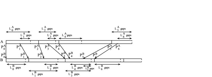
Figure 7: Illustration of the mapping of the first percolation into the other using the induction procedure. The blue and red segments of blocks are depicted as in Figure 5. In this example, $L_{0}^{A}\geq L_{0}^{B},L_{1}^{A}\leq L_{1}^{B},\ldots.$

Let us show the above induction (see Figure 7). For $j=0$, the event $E_{0}:=E_{0}^{A}\cap E_{0}^{B}$ [recall (4)], $P_{j}^{A}=P_{j}^{B}=0$, $T_{0}$ is just defined on $0\in A$ by $T_{0}(0)=0$ and, on the event $E_{0}$, we let $L_{0}^{A}$ be the length of the first blue segment of $A$ and $L_{0}^{B}$ be the length of the first blue segment of $B$. It is easy to see that all of the properties stated above hold.

Now, suppose that $\{E_{i}\}_{i=0}^{j-1}$ have occurred and that we have already constructed the above random variables up to stage $j-1$ with the above properties. We condition on $\bigcap_{i=0}^{j-1}E_{i},P_{j-1}^{A},P_{j-1}^{B},T_{j-1},L_{j-1}^{A}$ and $L_{j-1}^{B}$. There are two cases to consider:

1. $L^{B}_{j-1}\geq L^{A}_{j-1}$ [note that this also implies $L^{B}_{j-1}\geq K$, by property (iii) above]. Let $Q_{j}^{A}:=s_{L^{A}_{j-1}}(P_{j-1}^{A})$, $Q_{j}^{B}:=s_{L^{B}_{j-1}}(P_{j-1}^{B})$. By the induction assumption, the segment $A\cap[P_{j-1}^{A},Q_{j}^{A}]$ translated to start at $0$ is distributed $\mathcaligr{L}_{L^{A}_{j-1}}^{\mathrm{blue}}$ and the segment $B\cap[P_{j-1}^{B},Q_{j}^{B}]$ translated to start at $0$ is distributed $\mathcaligr{L}_{L^{B}_{j-1}}^{\mathrm{blue}}$. Let $P_{j}^{A}$ denote the end of the red segment which follows $A\cap[P_{j-1}^{A},Q_{j}^{A}]$, that is,

   $$P_{j}^{A}:=\min\{x\in A|x>Q_{j}^{A},g(s_{i}(x))\leq M\mbox{ for all $0\leq i\leq K-1$}\},$$

   and let $L^{A}_{j}$ be the number of short gaps of $A$ after $P_{j}^{A}$, that is,

   $$L^{A}_{j}:=\max\{N|g(s_{i}(P_{j}^{A}))\leq M\mbox{ for all $0\leq i\leq N-1$}\}.$$

   Note that, by definition of $P_{j}^{A}$, we have $L^{A}_{j}\geq K$. We now invoke Theorem 5.7 with the following parameters: $U^{1}$ is the segment $A\cap[P_{j-1}^{A},Q_{j}^{A}]$ translated to start at $0$, $V$ is the segment $A\cap[Q_{j}^{A},P_{j}^{A}]$ translated to start at $0$ and $U^{2}$ is the segment $B\cap[P_{j-1}^{B},Q_{j}^{B}]$ translated to start at $0$ ($W$ is then $A\cap[P_{j-1}^{A},P_{j}^{A}]$ translated to start at $0$). The theorem gives us $S$, which is a stopping time for $U^{2}$ conditioned on $U^{1}$ and $V$. Let $E_{j}$ be the event $E$ of that theorem, that is,

   $$E_{j}:=\biggl{\{}S\leq\max\biggl{(}\frac{K}{2},\frac{L^{A}_{j-1}}{\sqrt{\log_{2}n}}\biggr{)}\biggr{\}}.$$

   According to part (ii) of that theorem, on the event $E_{j}$, we have a Markov rough isometry $\widetilde{T}_{j}\dvtx W\to U^{2}\cap[0,s_{S}(0)]$ with constants $(M,F,R)$. Let $P_{j}^{B}:=s_{S}(P_{j-1}^{B})$ and $L_{j}^{B}:=L_{j-1}^{B}-S$, and note that, on the event $E_{j}$, $L_{j}^{B}\geq\max(L^{A}_{j-1},K)-S\geq\frac{1}{2}\max(L^{A}_{j-1},K)\geq\frac{K}{2}$. Finally, to construct $T_{j}$ we “concatenate” $T_{j-1}$ and $\widetilde{T}_{j}$, that is,

   $$T_{j}(x):=\cases{T_{j-1}(x),&\quad$x\in A,x\leq P_{j-1}^{A}$,\cr\widetilde{T}_{j}(x-P_{j-1}^{A})+P_{j-1}^{B},&\quad$x\in A,P_{j-1}^{A}\leq x\leq P_{j}^{A}$.}$$

   Note that $T_{j}$ is indeed a Markov rough isometry with constants $(M,F,R)$ since $T_{j-1}$ and $\widetilde{T}_{j}$ are, and since there is a unique preimage to $P_{j-1}^{B}$. Also note that by Lemma 5.4, we have that, conditioned on $E_{j}$ and $S$, the distribution of $B\cap[P_{j}^{B},\infty)$ is that of a Bernoulli percolation with $L^{B}_{j}$ initial short gaps. Hence, $E_{j}$, $P_{j}^{A}$, $P_{j}^{B}$, $T_{j}$, $L_{j}^{A}$ and $L_{j}^{B}$ satisfy the requirements of the induction step.

2. $L^{A}_{j-1}\geq L^{B}_{j-1}$. The induction step in this case is performed in the same way as in the first case, but with the roles of $A$ and $B$ interchanged and using part (iii) of Theorem 5.7 instead of part (ii).

All that remains is to prove Theorem 5.7, which we now do. Proof of Theorem 5.7 We divide the proof into several parts:

1. First, consider $U^{1}$. Applying the algorithm of Lemma 5.5 to $U^{1}$ with $Z=F$, we obtain a division of $U^{1}$ into $Y$ subsegments. Denote these by $U^{1}_{1},\ldots,U^{1}_{Y}$. If we let $\Omega_{1}:=\{Y\leq\frac{3L_{1}}{F}\}$, then, by Lemma 5.5, there exists a $c>0$ such that

   $$\mathbb{P}(\Omega_{1}^{c})\leq e^{-cL_{1}}\leq e^{-c{K}/{2}}.$$

2. Now, consider $V$. Let $X$ be the number of long gaps in $V$ and let $\{b_{i}\}_{i=1}^{X}$ be their lengths. Let $\Omega_{2}:=\{X\leq\frac{1}{8}\sqrt{\log_{2}n}\}$ and $\Omega_{3}:=\{\sum_{i=1}^{X}b_{i}\leq 3\log_{2}n\}$. Then, by Lemma 5.3, for some $\beta,\gamma>0$,

   $$\mathbb{P}(\Omega_{2}^{c}) \leq o\biggl{(}\frac{1}{n^{1+\beta}}\biggr{)},$$

   $$\mathbb{P}(\Omega_{3}^{c}) \leq o\biggl{(}\frac{1}{n^{1+\gamma}}\biggr{)}.$$

3. We continue to consider $V$. Let $(z_{i})_{i=1}^{X}\subseteq V$ be the starting points of the long gaps in $V$ ($z_{1}=0$), that is, $g(z_{i})>M$ for all $i$. They divide $V$ into $X-1$ subsegments, $V^{1}:=V\cap[s(z_{1}),z_{2}],\ldots,V^{X-1}:=V\cap[s(z_{X-1}),z_{X}]$. By the (structure) Lemma 5.2, we know that each subsegment conditioned on its length and translated to start at $0$ is distributed as a blue segment of that length. Let us again employ the algorithm of Lemma 5.5 with $Z=F$ to each of these subsegments to divide them further into “sub-subsegments.” Let $Y_{i}$ be the number of sub-subsegments in the division of $V^{i}$ and denote them by $(V^{i}_{j})_{j=1}^{Y_{i}}$ (for each $j$, $V^{i}_{j}\subseteq V^{i}$). Let $\Omega_{4}:=\{\sum_{i=1}^{X-1}Y_{i}\leq\frac{K}{20}\}$. To bound $\sum_{i=1}^{X-1}Y_{i}$, we consider the blue segment $\widetilde{V}$ obtained from $V$ by deleting all of its long gaps and translating to start at $0$. More precisely, write $V^{i}=(y^{i}_{0},\ldots,y^{i}_{N^{i}})$, where $N_{i}$ is the number of gaps in $V^{i}$, let $\widetilde{V}^{i}:=(0,y^{i}_{1}-y^{i}_{0},\ldots,y^{i}_{N^{i}}-y^{i}_{0})=:(0,\widetilde{y}^{i}_{1},\ldots,\widetilde{y}^{i}_{N^{i}})$ and then define

   $$\widetilde{V} := \Biggl{(}\underbrace{0,\widetilde{y}^{1}_{1},\ldots,\widetilde{y}^{1}_{N^{1}}}_{\widetilde{V}^{1}},\underbrace{\widetilde{y}^{2}_{1}+\widetilde{y}^{1}_{N^{1}},\ldots,\widetilde{y}^{2}_{N^{2}}+\widetilde{y}^{1}_{N^{1}}}_{\mathrm{Translated}\ \widetilde{V}^{2}},\ldots,$$

   $$\hskip 35.0pt\underbrace{\widetilde{y}^{X-1}_{1}+\sum_{j=1}^{X-2}\widetilde{y}^{j}_{N^{j}},\ldots,\widetilde{y}^{X-1}_{N^{X-1}}+\sum_{j=1}^{X-2}\widetilde{y}^{j}_{N^{j}}}_{\mathrm{Translated}\ \widetilde{V}^{X-1}}\Biggr{)}.$$

   $\widetilde{V}$ is a blue segment as a concatenation of many independent blue segments. We also apply the algorithm of Lemma 5.5 to $\widetilde{V}$ with $Z=F$ to divide it into $\widetilde{Y}$ subsegments. It is clear from the algorithm that $\widetilde{Y}\leq\sum_{i=1}^{X-1}Y_{i}$, but since, in the passage from $V$ to $\widetilde{V}$, we only removed $X$ long gaps, one must also check that

   $$\sum_{i=1}^{X-1}Y_{i}\leq\widetilde{Y}+X.$$ (7)

   We recall that $N$ is the number of gaps in $V$ and note that by the (structure) Lemma 5.2, $N\leq 1+K(X-1)\leq KX$. We wish to show that

   $$\mathbb{P}\biggl{(}\widetilde{Y}>\frac{K}{21}\biggr{)}=o\biggl{(}\frac{1}{n^{1+\beta}}\biggr{)}.$$ (8)

   For this, we divide the problem into three cases:

   • $N>\frac{KF}{70}$. This implies that $X>\frac{F}{70}>\frac{1}{8}\sqrt{\log_{2}n}$, which we know, by (2), to have probability at most $o(\frac{1}{n^{1+\beta}})$.

   • $\frac{KF}{70}\geq N>\frac{K}{21}$. Applying Lemma 5.5, we have

     $$\mathbb{P}\biggl{(}\widetilde{Y}>\frac{K}{21},\frac{KF}{70}\geq N>\frac{K}{21}\biggr{)} \leq \mathbb{P}\biggl{(}\widetilde{Y}>\frac{3N}{F},\frac{KF}{70}\geq N>\frac{K}{21}\biggr{)}$$

     $$\leq \mathbb{E}e^{-cN}\mathbf{1}_{({KF}/{70}\geq N>{K}/{21})}\leq e^{-c{K}/{21}}.$$

   • $N\leq\frac{K}{21}$. On this event, we certainly must have $\widetilde{Y}\leq\frac{K}{21}$,

   and (8) follows. Using (2), (7) and (8), we deduce, for large enough $n$, that

   $$\mathbb{P}(\Omega_{4}^{c})\leq\mathbb{P}\biggl{(}\widetilde{Y}>\frac{K}{21}\biggr{)}+\mathbb{P}(\Omega_{2}^{c})=o\biggl{(}\frac{1}{n^{1+\beta}}\biggr{)}.$$

4. We now consider the gap sequence $G:=G^{U^{2}}=(g_{i})_{i=1}^{L_{2}}$ of $U^{2}$ and the sequence $\widetilde{G}:=(g_{i})_{i=Y}^{\infty}$ ($Y$ was defined in the first item of the proof), where we have extended the sequence to be infinite by concatenating an i.i.d. sequence $(g_{i})_{i=L_{2}+1}^{\infty}$ of $\operatorname{Geom}_{\leq M}(\frac{1}{2})$ random variables, independent of everything else. We apply Lemma 5.6 to $\widetilde{G}$ with the parameters $m=X,a_{i}:=\lceil\frac{b_{i}}{M}\rceil$ (recall that $\{b_{i}\}_{i=1}^{X}$ are the lengths of the long gaps of $V$) and $d_{i}=Y_{i}-1$, to obtain $Z$, the first valid position along $\widetilde{G}$ (“valid position” was defined in the lemma). Let $\Omega_{5}:=\{Z\leq K^{{3}/{4}}\}$. Let $s:=\sum_{i=1}^{X}a_{i}$ and choose $a:=2^{{1}/{4}\sqrt{\log_{2}n}}$. Then, by the lemma,

   $$\mathbb{P}(Z>\lceil a2^{s}\rceil|X,\{b_{i}\}_{i=1}^{X},\{Y_{i}\}_{i=1}^{X-1})\leq e^{-{a}/{X^{2}}}.$$

   Since, on the events $\Omega_{2}$ and $\Omega_{3}$, we have $s\leq\frac{3\log_{2}n}{M}+X\leq\frac{9}{20}\sqrt{\log_{2}n}$, we obtain, for large enough $n$,

   $$\mathbb{P}(Z>K^{{3}/{4}},\Omega_{2},\Omega_{3}|X,\{b_{i}\}_{i=1}^{X},\{Y_{i}\}_{i=1}^{X-1})$$

   $$\qquad\leq\mathbb{P}(Z>\lceil a2^{s}\rceil,\Omega_{2},\Omega_{3}|X,\{b_{i}\}_{i=1}^{X},\{Y_{i}\}_{i=1}^{X-1})\leq e^{-{a}/{X^{2}}}.$$

   Hence, $\mathbb{P}(\Omega_{5}^{c})=o(\frac{1}{n^{1+\beta}})+o(\frac{1}{n^{1+\gamma}})$.

5. Finally, we construct the required time $S$, event $E$ and Markov rough isometries $T_{1}$ and $T_{2}$. We define

   $$S:=Y+Z+X+\sum_{i=1}^{X-1}(Y_{i}-1)=Y+Z+1+\sum_{i=1}^{X-1}Y_{i}.$$

   We note that, just as in Remark 5.1, conditioned on $W$ [in particular, on $Y,X$ and $(Y_{i})_{i=1}^{X-1}$], the time $S$ is a stopping time for $U^{2}$. We define the event

   $$\widetilde{E}:=\Omega_{1}\cap\Omega_{2}\cap\Omega_{4}\cap\Omega_{5}.$$

   Note that, by the previous calculations, $\mathbb{P}(\widetilde{E}^{c})=o(\frac{1}{n^{1+\delta}})$ for some $\delta>0$. On the event $\widetilde{E}$, we have

   $$S\leq\frac{3L_{1}}{F}+K^{{3}/{4}}+1+\frac{K}{20}\leq\max\biggl{(}\frac{K}{2},\frac{L_{1}}{\sqrt{\log_{2}n}}\biggr{)},$$

   hence the event $E$ of the theorem satisfies $E\supseteq\widetilde{E}$. On the event $E$, we now construct $T_{1}$ (see Figure 8). $T_{2}$ is constructed

   

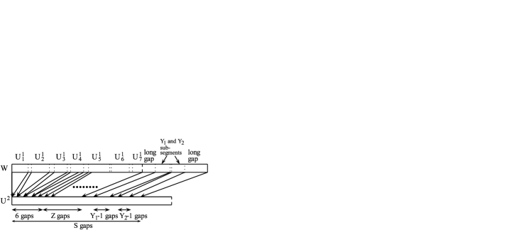
   Figure 8: Illustration of the constructed rough isometry. In the picture, $Y=7$ and $X=3$. When mapping $U^{1}$ to $U^{2}$, we start mapping points one-to-one rather than many-to-one, starting from subsegment $j_{0}:=4$.

   analogously, using the fact that $R=F$. First, we define $T_{1}$ on the points of $U^{1}$ in such a way that $T_{1}(x^{1}_{L_{1}})=x^{2}_{Y+Z}$. Note that, on the event $E$,

   $$L_{1}-Y = L_{1}-S+Z+1+\sum_{i=1}^{X-1}Y_{i}$$

   $$\geq L_{1}-\max\biggl{(}\frac{K}{2},\frac{L_{1}}{\sqrt{\log_{2}n}}\biggr{)}+Z\geq Z$$

   since $L_{1}\geq\frac{K}{2}$. We start mapping the points of $U^{1}$ to $U^{2}$ according to the subsegment $U^{1}_{j}$ that the point of $U^{1}$ is in. More precisely, we consider all of the points of $U^{1}$ in order and if a point $x^{1}_{i}\in U^{1}_{j}$, then we define $T(x^{1}_{i}):=x^{2}_{j-1}$ (where $x^{2}_{0}$ is defined to be $0$). By the definition of the subsegments $(U^{1}_{j})_{j=1}^{Y}$, for all $j$, we will have $\max T^{-1}(x^{2}_{j-1})-\min T^{-1}(x^{2}_{j-1})\leq F$, as required. Furthermore, since $x^{1}_{i+1}-x^{1}_{i}\leq M$ for all $i$ and $x^{2}_{j+1}-x^{2}_{j}\geq 1$, we will not expand or contract any distance by more than $M$. We stop mapping in this way when we reach a point $x^{1}_{i_{0}}$ belonging to $U^{1}_{j_{0}}$ which satisfies $L_{1}-i_{0}=Y+Z-(j_{0}-1)$. Such a point must be reached for some $0\leq i_{0}\leq L_{1}$, by (5). From this point on, we map the points sequentially as follows: $T(x^{1}_{i_{0}+l}):=x^{2}_{j_{0}-1+l}$ for $0\leq l\leq L_{1}-i_{0}$. As before, no distances are expanded or contracted by more than $M$.

   We continue to define $T_{1}$ at the points of $W$ which follow $x^{1}_{L_{1}}$ (the translated points of $V$). Recalling that $(z_{i})_{i=1}^{X}\subseteq V$ are the starting points of the long gaps in $V$ (the corresponding points of $W$ are $z_{i}+x^{1}_{L_{1}}$), we construct the remainder of the mapping $T_{1}$ by induction on $1\leq j\leq X$. Note that since $z_{1}=0$, we have already defined $T_{1}(z_{1}+x^{1}_{L_{1}})=x^{2}_{Y+Z}$. Define further $T_{1}(s(z_{1}+x^{1}_{L_{1}})):=x^{2}_{Y+Z+1}$; this is the $j=1$ stage. Note that by the definition of $Z$, we did not contract the gap of $W$ by more than $M$ (and, of course, we did not expand it since we mapped to a short gap).

   For $2\leq j\leq X$, let $R_{j}:=\sum_{i=1}^{j-1}Y_{i}$. Suppose that we have already constructed the mapping $T_{1}$ to be a Markov rough isometry with constants $(M,F,R)$ from $W\cap[0,s(z_{j-1}+x^{1}_{L_{1}})]$ to $U^{2}\cap[0,x^{2}_{Y+Z+1+R_{j-1}}]$ in such a way that $T_{1}(s(z_{j-1}+x^{1}_{L_{1}}))=x^{2}_{Y+Z+1+R_{j-1}}$ and that it is the only source of $x^{2}_{Y+Z+1+R_{j-1}}$. Recall that we have divided the subsegment $V^{j-1}$ into sub-subsegments $(V^{j-1}_{k})_{k=1}^{Y_{j-1}}$ and consider a point $x_{l}\in W\cap[s(z_{j-1}+x^{1}_{L_{1}}),z_{j}+x^{1}_{L_{1}}]$. There then exists some $k$ such that $x_{l}-x^{1}_{L_{1}}\in V^{j-1}_{k}$. Define $T_{1}(x_{l}):=x^{2}_{Y+Z+1+R_{j-1}+(k-1)}$. Note that this is consistent with the definition of $s(z_{j-1}+x^{1}_{L_{1}})$, that $T_{1}(z_{j}+x^{1}_{L_{1}})=x^{2}_{Y+Z+R_{j}}$, that by the choice of the sub-subsegments for each point $x^{2}_{l}\in U^{2}\cap[x^{2}_{Y+Z+1+R_{j-1}},x^{2}_{Y+Z+R_{j}}]$, we have $\max T_{1}^{-1}(x^{2}_{l})-\min T_{1}^{-1}(x^{2}_{l})\leq F$, and that since we are mapping gaps not larger than $M$ to gaps of size between $1$ and $M$, no distance was expanded or contracted by more than $M$ (whenever two points are mapped to different images). Finally, define $T_{1}(s(z_{j}+x^{1}_{L_{1}})):=x^{2}_{Y+Z+1+R_{j}}$. Again, by the choice of $Z$, this mapping did not contract the gap of $W$ by more than $M$ (and, of course, we did not expand it since we mapped to a short gap). Continuing this procedure until $j=X$ completes the construction of the map $T_{1}\dvtx W\to U^{2}\cap[0,x^{2}_{S}]$, as required.

References

- (1) {bmisc}[auto:springertagbib-v1.0] \bauthor\bsnmAbért, \bfnmM.\binitsM. (\byear2008). \bhowpublishedPrivate communication. Available at http://www.math.uchicago.edu/~abert/research/asymptotic.html. \endbibitem
- (2) {bbook}[mr] \bauthor\bsnmAlon, \bfnmNoga\binitsN. and \bauthor\bsnmSpencer, \bfnmJoel H.\binitsJ. H. (\byear2000). \btitleThe Probabilistic Method, \bedition2nd ed. \bpublisherWiley, \baddressNew York. \bidmr=1885388 \endbibitem
- (3) {barticle}[mr] \bauthor\bsnmAngel, \bfnmOmer\binitsO. and \bauthor\bsnmBenjamini, \bfnmItai\binitsI. (\byear2007). \btitleA phase transition for the metric distortion of percolation on the hypercube. \bjournalCombinatorica \bvolume27 \bpages645–658. \bidmr=2384409 \endbibitem
- (4) {bmisc}[unstr] \bauthor\bsnmBenjamini, \bfnmI.\binitsI. (\byear2005). \bhowpublishedPrivate communication. \endbibitem
- (5) {barticle}[mr] \bauthor\bsnmDelmotte, \bfnmThierry\binitsT. (\byear1999). \btitleParabolic Harnack inequality and estimates of Markov chains on graphs. \bjournalRev. Mat. Iberoamericana \bvolume15 \bpages181–232. \bidmr=1681641 \endbibitem
- (6) {bincollection}[mr] \bauthor\bsnmGromov, \bfnmM.\binitsM. (\byear1981). \btitleHyperbolic manifolds, groups and actions. In \bbooktitleRiemann Surfaces and Related Topics: Proceedings of the 1978 Stony Brook Conference (State Univ. New York, Stony Brook, N.Y., 1978). \bseriesAnnals of Mathematics Studies \bvolume97 \bpages183–213. \bpublisherPrinceton Univ. Press, \baddressPrinceton, NJ. \bidmr=624814 \endbibitem
- (7) {barticle}[mr] \bauthor\bsnmKanai, \bfnmMasahiko\binitsM. (\byear1985). \btitleRough isometries, and combinatorial approximations of geometries of noncompact Riemannian manifolds. \bjournalJ. Math. Soc. Japan \bvolume37 \bpages391–413. \bidmr=792983 \endbibitem
- (8) {barticle}[mr] \bauthor\bsnmKozma, \bfnmGady\binitsG. (\byear2007). \btitleThe scaling limit of loop-erased random walk in three dimensions. \bjournalActa Math. \bvolume199 \bpages29–152. \bidmr=2350070 \endbibitem
- (9) {bmisc}[auto:springertagbib-v1.0] \bauthor\bsnmKozma, \bfnmG.\binitsG. (\byear2006). \bhowpublishedPrivate communication. \endbibitem