Globular Cluster Abundances from High-Resolution Integrated Light Spectra, I: 47 Tuc

Abstract

We describe the detailed chemical abundance analysis of a high-resolution (R$\sim$35,000), integrated-light (IL), spectrum of the core of the Galactic globular cluster 47 Tuc, obtained using the du Pont echelle at Las Campanas. This is the first paper describing the abundance analysis of a set of Milky Way clusters of which we have obtained integrated light spectra; we are analyzing these to develop and demonstrate an abundance analysis strategy that can be applied to spatial unresolved, extra-galactic clusters.

We have computed abundances for Na, Mg, Al, Si, Ca, Sc, Ti, V, Cr, Mn, Fe, Co, Ni, Cu, Y, Zr, Ba, La, Nd and Eu. For an analysis with the known color-magnitude diagram (cmd) for 47 Tuc we obtain a mean [Fe/H] value of $-$0.75 $\pm$0.026$\pm$0.045 dex (random and systematic error), in good agreement with the mean of 5 recent high resolution abundance studies, at $-$0.70 dex. Typical random errors on our mean [X/Fe] ratios are 0.07–0.10 dex, similar to studies of individual stars in 47 Tuc. Only Na and Al appear anomalous, compared to abundances from individual stars: they are enhanced in the IL spectrum, perhaps due to proton burning in the most luminous cluster stars.

Our IL abundance analysis with an unknown cmd employed theoretical Teramo isochrones; however, the observed frequency of AGB bump stars in 47 Tuc is approximately three times higher than theoretical predictions, so we adopt zero-point abundance corrections to account for this deficiency. The spectra, alone, provide mild constraints on the cluster age, ruling-out ages younger than $\sim$2 Gyr. However, when we include theoretical IL B$-$V colors and metallicity derived from the Fe I lines, the age is constrained to 10–15 Gyr and we obtain [Fe/H]=$-$0.70$\pm$0.021$\pm$0.052 dex.

We also find that trends of IL Fe line abundances with equivalent width and excitation potential can constrain the horizontal branch morphology of an unresolved cluster, as well as age. Lastly, our spectrum synthesis of 5.4 million TiO lines indicates that the 7300–7600Å TiO window should be useful for estimating the effect of M giants on the IL abundances, and important for clusters more metal-rich than 47 Tuc.

1 Introduction

Detailed high-resolution chemical abundance analysis of individual stars in Galactic globular clusters (GCs) has been pursued for 30 years (e.g. Cohen 1978; Pilachowski, Canterna & Wallerstein 1980). Such abundance studies are a critical tool for probing the chemical evolution of the Galaxy as well as stellar evolution up the giant branch (e.g. Sneden et al. 1991; Briley, Smith & Lambert 1994) and complemented earlier work on nearby field stars (e.g. Wallerstein 1962, Luck & Bond 1985). Unfortunately, similar studies have never been possible in other galaxies beyond the Local Group dwarfs, as even the brightest red giant branch stars are too faint to be seen in distant galaxies. Indeed, only recently have abundances of individual GC red giant stars in the closest members of the Local Group become available (e.g. Johnson, Ivans & Stetson 2006; Letarte et al. 2006).

For extra-galactic GCs, integrated-light metallicities have been estimated for systems ranging from M31 to the Virgo cluster of galaxies, using broad-band photometric colors (e.g. Forte, Strom & Strom 1981; Geisler et al. 1996) and low-resolution spectra (e.g. Racine, Oke & Searle 1978; Brodie & Huchra 1990). The low resolution spectra typically employ the “Lick” index system (e.g. Faber 1973), which is based on correlations between strong absorption features at low resolution and detailed abundances obtained for individual Galactic GC stars, at high spectral resolution. All of these indices contain numerous lines from several elements, although many are dominated by particular species that can be empirically calibrated to give very approximate composition information (e.g. the Mg₂ index can be calibrated for approximate [Mg/Fe] or [$\alpha$/Fe]). An example of this is the study of NGC 5128 by Peng, Ford & Freeman (2004); in this case even quite crude composition information provides a powerful investigative tool. Results from such studies include the discovery of bimodal GC metallicity/color distribution in extra-galactic systems (e.g. Elson & Santiago 1996; Whitmore et al. 1995), reminiscent of the bimodal GCs in the Galaxy (e.g. Zinn 1985).

Because of their relative homogeneity, ages ($>>$ 1 Gyr), and high luminosity, GCs can be used to probe the chemical evolution history of galaxies. The most luminous GCs presumably only trace the major star forming events, including mergers. As indicated above, even basic metallicity provides interesting information for comparison with the Milky Way galaxy. However, detailed chemical composition of GCs could potentially provide a plethora of information on galaxy evolution, because the chemical elements are produced by a variety of stars, with varying sensitivity to stellar mass and metallicity.

We are developing a method for measuring detailed chemical abundances of GCs using high resolution spectra of their integrated light (McWilliam & Bernstein 2002; Bernstein & McWilliam 2005). Due to low the velocity dispersions of GCs ($\sigma$$\sim$1–20 Km/s), the intrinsic line widths of the integrated light spectra are small enough that individual lines are well resolved and blending is not much more problematic than for individual red giant stars. In Figure 1, we demonstrate this point with a plot of velocity dispersion as a function of M_v for Galactic GCs. Also shown in that figure is the line width parameter, $R$=$\lambda$/FWHM, that corresponds to the plotted velocity dispersions. It is clear from this plot that spectral resolutions of R$\geq$10,000 are necessary to resolve the spectral lines in even the brightest GCs; R$\geq$30,000 is necessary for the average Galactic GCs. With spectrograph resolving power somewhat larger than these values of $R$, line profiles can be fully characterized. These narrow line widths are in stark contrast to those of giant galaxies (elliptical and spiral), which have velocity dispersions in the range 100-300 Km/s (e.g. Faber & Jackson 1976) and line width parameters, $R$, of order 1,000–3,000. The Lick system, which has been used to measure the ages and metallicities of stellar systems from GCs to giant elliptical galaxies, is based on spectra with resolving power $\lambda/\Delta\lambda\sim$600 (e.g. Faber et al. 1985; Worthey et al. 1994; Trager 2004). While the sampling of this index system is justified for faint giant galaxies, a low resolution system such as this does not utilize the available information for bright GCs. As we show in this paper, it is possible to use high dispersion integrated-light spectra of GCs to reveal a wealth of abundance information from the weak lines of numerous elements that are lost in low resolution, low S/N, spectra. Indeed, high resolution spectra, employing diagnostics similar to those used in the spectral analysis of single stars, can be used to break the age-metallicity degeneracy that is troublesome at low spectral resolution.

In this paper we demonstrate the possibilities and some of the practical challenges for using IL spectra of GCs to measure detailed chemical composition. This analysis holds significant potential for galaxy evolution constraints. Due to the high luminosity of GCs, high-resolution spectra of sufficient quality can be obtained for GCs at extra-galactic distances and used to probe the chemical evolution of distant galaxies. The luminosities of the brightest GCs are comparable to young supergiant stars, for which abundances have been measured in Local Group galaxies (e.g. Venn et al. 2001; Kaufer et al. 2004) using spectra from large telescopes. However, unlike short-lived, supergiant stars that reveal only recent gas compositions, GCs ages cover the full range of galactic history.

In particular, this paper focuses on the analysis of one cluster (NGC 104) from a sample of “training set” clusters that we have observed and analyzed with the goal of developing and demonstrating a technique for abundance analysis of a single age, chemically homogeneous, stellar population. Our “training set” is comprised of a sample of Galactic and LMC GCs. Of these, the Galactic GCs are well studied, with photometric and detailed abundance studies of individual stars in the literature. Because they are well studied, distance and reddening parameters are readily available for use in our analysis, as are “fiducial” abundances obtained from individual stars which we can use to check our final abundance results. We begin with the luminous GC 47 Tuc ([Fe/H]$\sim$$-$0.7 e.g. Carretta et al. 2004) for several reasons. 47 Tuc is very bright, making IL spectra easy to obtain, and it has very low reddening (near E(B$-$V)=0.03 magnitudes), which will be useful for the analysis. Furthermore, the relatively high metallicity results in easy visibility of lines from many elements.

2 Observations and Reductions

We acquired high resolution, integrated light spectra of our “training set” GCs using the echelle spectrograph on the Las Campanas 2.5m du Pont telescope during lunar dark time in July 2000. We limit the discussion here to 47 Tuc; the full training set will be discussed in a later paper (Bernstein et al 2008). The observations were facilitated by a modification to the telescope guider program, kindly performed by S. Shectman, which enabled a uniform scan of the echelle slit across a $32\times 32$ arcsecond square region of sky, from $16^{\prime\prime}$ South-West to $16^{\prime\prime}$ North-East of the field center. Since the cluster regions were scanned once per exposure, clear skies were necessary to ensure an unbiased weighting of the cluster light. The entire 1$\times$4 arcsecond echelle slit was filled with cluster light during these scans of the cluster core, and significant sky flux outside the telluric emission lines was only detected near twilight. Nevertheless sky exposures were taken separately to allow subtraction of the sky signal from the science exposures. We obtained three exposures of roughly 1 hour each on the 47 Tuc core and five 20 minute exposures on the sky.

We performed the basic data reduction steps using the echelle package in IRAF, including the routines for overscan, bias subtraction, and flat-field division. The sky spectra were scaled and subtracted from the individual integrated-light exposures using simple arithmetic routines.

The mean line widths of the Th-Ar comparison spectra, at 2.6 pixels, correspond to a spectral resolving power ($R$=$\lambda$/FWHM) of 34,760, but this value varies over the CCD by $\sigma$$\sim$4%, due to focus variations in the camera optics.

While our du Pont echelle integrated-light spectra cover the wavelength interval 3700–7800Å, the useful range is limited at the red end, because the orders are too close in the cross dispersion direction for good extraction, and due to blending with telluric absorption lines. The utility of the blue side is limited by the reduced flux and increased line blending. Thus, the useful wavelength coverage of our 47 Tuc spectrum is from $\sim$5000 to 7570Å.

In spectra from the du Pont echelle, the wings of adjacent orders in the red region of the spectrum ($\lambda$$\geq$6000Å) overlap slightly, making it difficult to identify the local scattered-light background levels; this problem is particularly acute when the source fills the slit, as in our observations, thus widening the order profile relative to the spectrum of a point source. It was therefore necessary to estimate the scattered-light background using an empirical model. To do so, we used the two-dimensional image of a spectrum of a bright red giant star, taken with the smallest possible slit (0.75$\times$0.75 arcseconds square). The bright giant star flux distribution is similar to that of the integrated-light spectrum of an old cluster like 47 Tuc. This short slit gave well separated spectral orders, with much less inter-order light in the red region (where the orders are closest) than for the cluster integrated-light spectra. The relatively flat bottomed troughs of the short slit inter-order light suggests scattered-light rather than overlapping wings of adjacent orders. In Figure 2 we show a comparison of the GC spectral orders and the orders of the short slit star spectrum; essentially, we use the ratio of total flux in an order to the inter-order flux for the short slit spectrum to define the scattered light in the GC spectrum. It is notable that the scaled short slit inter-order flux in Figure 2 is consistent with the GC inter-order light for column positions less than 910 pixels. We found that the scattered light is roughly $\sim 6$% of the total stellar flux, in a given order, and is a function of wavelength redder than $5000$Å. To measure the total flux in each order of the science spectra, we extracted the orders using the IRAF echelle routine apall with wide apertures and without background subtraction. The scattered light flux in the model was scaled according to the total flux and the size of the extraction aperture and then subtracted from the object spectrum.

We noticed that the scattered light followed approximately the continuous flux distribution of the object spectrum, in the wavelength and cross-dispersion directions. To gain a greater understanding of the scattered-light, we constructed a simple analytical model for the scattering and performed numerical experiments to try to mimic the shape of the scattered-light along the dispersion and cross-dispersion directions on the CCD. This analytical model included only two parameters: the amount of light scattered and a scattering scale length, based on a Gaussian scattered-light distribution. Our results indicated that the scattered-light scale length was approximately 200 pixels. At any given pixel, the scattered light therefore came from a $\sim$10–20 Å region in the dispersion direction and roughly 8 or 9 echelle orders in the cross-dispersion direction. We used only the empirical scattered-light model derived from the bright star spectrum through the (0.75$\times$0.75 arc sec) short slit, not the analytical model, in the reduction of our science exposures.

Although the empirical scattered-light model appeared to work quite well for the red region of the spectrum, it did not always compare well with the measured scattered light in the blue, where the orders are well spaced and scattered light can be measured directly. We believe that this is because the scattered-light in the blue portion of the CCD was overwhelmed by scattered light from the bright red part of the spectrum; essentially, a small fraction of light scattered from the far red end of the spectrum could overwhelm the local scattered light between the blue spectral orders. In this case, a color difference between 47 Tuc and the star used for the empirical scattered-light model could make the empirical scattering model unreliable in the blue spectral region. Fortunately, the bluer orders of the IL spectrum are well separated, so that it is possible to measure the scattered light directly from the GC IL spectrum at these wavelengths. Therefore, we chose to use the scattered-light model only for the red orders where direct measurement of the scattered light was not possible.

After extraction and wavelength calibration, multiple exposures were combined using IRAF combine routines, with the crreject algorithm to eliminate pixels affected by cosmic ray strikes. For the purpose of measuring equivalent widths, we performed a simple normalization which removes the shape of the echelle blaze function from each order. The approximate shape of the blaze function was obtained by tracing the continuum flux of a bright giant in NGC 6397.

The S/N of the final spectrum is listed at three wavelengths in Table 1. Figures 3 and 4 show examples of the integrated-light spectra for GCs NGC 6397 and 47 Tuc. The average line widths of weak lines in the 5000–6500Å region of the 47 Tuc spectrum was measured at $\lambda$/FWHM=10,552, corresponding to an intrinsic $\lambda$/FWHM=11,065 once the spectrograph is taken into account. This line width indicates a velocity dispersion of 11.5 $\pm$0.2 Km/s, exactly equal to the result of Prior & Meylan (1993). From Figures 3 and 4 it is clear that abundance information for numerous elemental species is present in the high resolution integrated-light spectra, even for the relatively broad lines of 47 Tuc ($M_{\rm v}=-9.4$). Lines in GC integrated-light spectra are weaker and wider than for individual red giants, as a result of both the velocity broadening and the contribution of weaker lines from stars warmer and less luminous than the bright cluster giants. For this reason, greater S/N is required to obtain reliable abundances from integrated-light spectra than for individual red giant stars.

3 Analysis

Our goal in this paper is to explore strategies for the detailed abundance analysis of high-resolution IL spectra of GCs. To simplify the issues, we have used two methods that isolate different aspects of the problem to some degree. In the first method, we employ extant photometry of 47 Tuc and characterize the stellar populations by regions on the color-magnitude diagram (cmd). We begin by splitting the observed cmd into 27 regions (“boxes”), each with a small range in color and magnitude (see Figure 5). Our analysis then involves synthesizing a theoretical equivalent width (EW) for each spectral line for each of these boxes; we then combine these EWs, weighted by the continuum flux at each line and the total flux in each box to obtain a theoretical, flux weighted, IL EW. Obviously, it is not possible to employ this particular technique for very distant GCs that are spatially unresolved, because the cmds are not available; however, the method could be used to study GCs in nearby galaxies (e.g. M31) using space-based photometry.

The objective for this part of the investigation is to first, provide an independent abundance analysis of the integrated-light spectrum of 47 Tuc. The second, and more important, goal is to check our abundance analysis algorithms with minimal uncertainty in the adopted isochrone (or cmd). Thus, with this method we simply use the available information regarding the stellar population of the cluster to determine whether an IL spectrum synthesis method will, ultimately, be able to measure detailed chemical abundances from high resolution GC spectra. If IL spectra combined with the known color-magnitude diagrams of the clusters do not provide reliable abundance results, then it will certainly not be possible in the situation where a theoretical cmd must be assumed.

Our second method for analyzing IL spectra employs theoretical isochrones in place of the resolved cluster photometry. The accuracy of the derived abundances will clearly depend on how well the predicted isochrones match the luminosity function and temperatures of the stars in the clusters, and whether critical isochrone parameters can be constrained using the IL spectra alone. Since we do not know a priori what isochrone to use when analyzing unresolved GCs, we also develop diagnostics that enable us to constrain the isochrone parameters for the abundance analysis.

3.1 Measurement of the Spectral Lines

The first step in our analysis is uniform, repeatable measurement of the absorption line equivalent widths (EWs) in the 47 Tuc integrated-light spectrum. We measured the EWs by fitting the lines with Gaussian profiles using the semi-automated program GETJOB (see McWilliam et al. 1995a). We select our list of lines from those used by McWilliam & Rich (1994), McWilliam et al. (1995a,b), and Smecker-Hane & McWilliam (2002). There are fewer useful lines in globular cluster integrated-light spectra than for stars because the GC lines are broader and weaker than in the spectrum of individual red giant stars, and thus more difficult to measure. A complete list of our lines and EWs is given in Table 2. These line measurements are used for both of the analyses outlined below.

3.2 Integrated-Light Abundances with the Resolved CMD

As a preliminary step in developing a way to analyze unresolved globular clusters, we first consider the abundance analysis of the integrated light spectra using the available photometry for this resolved Milky Way cluster. The analysis involves two general stages: characterizing the stellar population in the cluster and synthesizing the strength of the spectral lines.

To begin the first stage of the analysis using the observed cmd, we divided the observed cmd into small boxes containing stars with similar photometric properties and we used standard relations to derive the flux-weighted “average” atmosphere parameters of the stars in each box. The boxes run from the main-sequence to the tip of the red giant branch, then along the horizontal branch/red clump region and the AGB. Two additional boxes are included for the blue straggler population. In this analysis, the mean stellar atmosphere parameters for stars in each box are estimated from the flux-weighted photometry. We then computed the absolute visual luminosities using reddening corrections and the distance modulus according to the equation

$$M_{\rm v}=V-(m-M).$$ (1)

The flux-weighted temperatures appropriate for each cmd box was computed using standard color-temperature relations. With initial estimates for [Fe/H], T_eff and $\log{g}$, the bolometric corrections, BC, were interpolated from the Kurucz grid (2002 unpublished). Bolometric magnitudes and luminosities were computed using the expressions

$$M_{\rm bol}=M_{\rm v}+BC$$ (2)

and

$$\log L/L{{}_{\odot}}=-0.4(M_{\rm bol}-M_{\rm bol\odot}),$$ (3)

where M_bol⊙ = 4.74. Gravities were computed using the expression

$$\log{g}=\log{g}_{\odot}+\log M/M_{\odot}-logL/L_{\odot}+4logT_{\rm eff}/T_{\rm eff\odot},$$ (4)

assuming a solar effective temperature of T_eff⊙=5777K, solar gravity of $\log{g}_{\odot}$=4.4378, and a mass for the cluster stars of 0.8M_⊙. We re-evaluated the specific gravity and bolometric corrections iteratively until convergence in $\log{g}$ was obtained to within 0.05 dex. Because 47 Tuc is old, and because our photometry included only a small portion of the main-sequence, we note that a negligible error in the final result would occur by assuming that the masses of all the stars in our cmd were equal to the turnoff mass. Microturbulent velocities were assumed to fit a linear regression through 1.00 Km/s for the sun at $\log{g}=4.44$, to 1.60 Km/s for Arcturus, at $\log{g}=1.60$ (Fulbright, McWilliam & Rich 2006):

$$\xi=\xi_{\odot}+\frac{(logg_{\odot}-logg)}{(logg_{\odot}-logg_{\alpha Boo})}(\xi_{\alpha Boo}-\xi_{\odot}).$$ (5)

Finally, stellar radii were computed for each cmd box according to the expression

$$R/R_{\odot}=(T_{\rm eff}\odot/T_{\rm eff})^{2}\sqrt[]{L/L_{\odot}}$$ (6)

These radii are needed in order to compute the total flux from each cmd box.

In Figure 5 we show the 47 Tuc V, B$-$V cmd (from Guhathakurta et al. 1992; Howell et al. 2000) for the central, 32$\times$32 arc seconds, scanned region. This region contains 4192 stars, which we have divided into 27 boxes; an additional 229 stars lay beyond the cmd boxes, but contribute insignificant flux to the total. As outlined above, we computed the flux-weighted V and B$-$V values for each cmd box, and used those values to calculate mean effective temperatures and gravities with the Alonso et al. (1999) color-temperature relations. Ancillary assumptions included [Fe/H]=$-$0.7 to compute the bolometric corrections and a turnoff mass of 0.8 M_⊙ for the gravity.

Because the B$-$V color–temperature relation and bolometric correction are sensitive to the stellar metallicity, it is necessary to adopt an initial [Fe/H] for the calculation of T_eff and BC. As a consequence the abundance analysis must be iterated until the adopted [Fe/H] value is consistent with the abundances derived from the Fe lines. Fortunately, the iterations converge extremely quickly: for 47 Tuc if we derive temperatures and BC values starting with an assumed metallicity of [Fe/H]=0.0 the first iteration obtains [Fe/H]=$-$0.65 from the lines, and the second iteration gives [Fe/H] within 0.02 dex of the self-consistent value. However, for other colors, such as V$-$I and V$-$K, the sensitivity of the color–T_eff relations and BC to metallicity are extremely small, so iteration is not required.

Table 3 provides the adopted stellar atmosphere parameters for the 47 Tuc BV cmd boxes. It is interesting to note that 50% of the V-band flux comes from giant stars at the red clump luminosity and brighter in this cluster (see Figure 5).

The second stage in the abundance analysis then involves spectrum synthesis to compute theoretical EWs of each line for each cmd box using a model atmosphere. The final EWs of lines in the integrated light of a cluster can then be computed by averaging the synthesized EWs together, weighted by the flux in each cmd box. In the line synthesis, the only adjustable parameter is the input abundances. All other parameters are fixed by the average stellar atmosphere parameters of the stars in each cmd box and the properties of the spectral line being calculated. The spectrum synthesis was performed using the program MOOG (Sneden 1973) modified to be called as a subroutine and to provide the continuum flux, $F_{c}$, for each line, within a larger program, ILABUNDS. Our code employs the alpha-enhanced Kurucz models (Castelli & Kurucz 2004) with the latest opacity distribution function (AODFNEW), linearly interpolated to arbitrary T_eff, logg and [Fe/H]. The flux-weighted, average line equivalent width for the integrated-light of the cluster was computed according to the following expression:

$$\overline{EW}=\frac{\sum_{i=1}^{n}EW_{i}w_{i}}{\sum_{i=1}^{n}w_{i}},$$ (7)

where $EW_{i}$ is the equivalent width of the line for a given box ($i$) and $w_{i}$ are the weights for each cmd box. We compute $w_{i}$ values using the radii, $R/R_{\odot}$, number of stars in the cmd box, $N_{*}$, and the emergent continuum fluxes (computed using MOOG) for the box, $F_{c}$, according to

$$w=R^{2}N_{*}F_{c}.$$ (8)

Abundances were determined by iteratively adjusting the assumed abundance in the line synthesis until the synthetic flux-weighted EW matched the observed IL EW for each line. We continued to iterate with small adjustments to the input abundance until the observed and predicted IL EWs agreed to one percent.

The use of an observed cmd limits the utility of this technique for detailed abundance analysis to globular clusters within the Local Group of galaxies, where ground or space-based telescopes are able to at least partially resolve individual cluster stars. While future 30 meter class telescopes, equipped with adaptive optics systems, may be able to resolve GC stars to even greater distances, ultimately our objective is to measure detailed composition from unresolved globular clusters. Analysis using observed photometry is a step toward that goal and confirms that the basic strategy of computing light weighted EWs is sound.

3.2.1 Iron Abundances

We begin our abundance study with the analysis for iron, because its numerous lines provide useful diagnostics of stellar atmosphere parameters. In our IL abundance analysis we employ the atmospheric parameters from the observed cmd listed in Table 3, the EWs and atomic parameters given in Table 2, and the prescription outlined above in §3.2. The atomic line parameters listed in Table 2 were taken from McWilliam & Rich (1994) and McWilliam et al. (1995). In Figures 6–8 we show diagnostic plots, using the abundances derived from the iron lines, similar to the diagnostics used for standard abundance analysis of single stars. Figure 6 shows that $\epsilon$(Fe) is independent of EW, which indicates that the assumed microturbulent velocity law that we have employed is sufficiently accurate; a positive slope would have suggested microturbulent velocities that are too low. The plot of $\epsilon$(Fe) versus excitation potential in Figure 7 is sensitive to the temperatures of the cmd boxes; the near-zero slope indicates that the adopted temperatures for the cmd boxes was approximately correct. Figure 8 shows that our iron abundances are independent of wavelength. This provides a general check on our abundance analysis, from consistency of the EW measurements to the mix of stellar types and the continuous opacity subroutines in our spectrum synthesis code. The increased upper envelope and scatter of iron abundances for lines redder than 7000Å led us to suspect that the scattered-light subtraction was flawed in this region, but it might instead be due to the effects of blends or poor $gf$ values. In general the trend of abundance with wavelength should provide a probe of the existence of sub-populations of varying temperature, such as hot stars on the blue horizontal giant branch.

From 102 measurements of 96 Fe I lines, we obtain a mean Fe I abundance of 6.77 $\pm$0.03 dex, with rms scatter about the mean of 0.26 dex. From 7 Fe II lines, we obtain a mean Fe II abundance of 6.73 $\pm$0.06 dex, with rms scatter about the mean of 0.16 dex,

The recent estimate of the solar iron abundance by Asplund, Grevesse & Sauval (2005) indicates a value of 7.45$\pm$0.05 dex, based on a 3D hydrodynamical solar model. Lodders (2003) found a solar iron abundance of 7.54 dex. While we believe that the Asplund et al. (2005) solar iron abundance value is probably the best current estimate, it is more reasonable for us to obtain a consistent and differential [Fe/H] value for 47 Tuc relative to the sun, by using the same lines, $gf$ values, grid of Kurucz 1D atmospheres and abundance analysis program for the sun and 47 Tuc. In this way, our Fe lines indicate a solar iron abundance of $\epsilon$(Fe)=7.52 for Fe I lines and $\epsilon$(Fe)=7.45 for Fe II lines. For [X/Fe] abundance ratios we adopt a solar iron abundance of $\epsilon$(Fe)=7.50, which is the average of many studies in recent years.

Our differential iron abundance values from Fe I and Fe II lines in 47 Tuc are $-$0.75$\pm$0.026 and $-$0.72$\pm$0.056 dex respectively, independent of adopted $gf$ values, where the uncertainties represent the 1$\sigma$ random error on the mean. We consider the 1$\sigma$ systematic uncertainties on our derived [Fe/H] values from the model atmospheres (0.03 and 0.03 dex for Fe I and II respectively), $gf$ scale zero-point (0.03 and 0.04 dex), and the effect of $\alpha$-enhancement (0.015 and 0.04 dex). We refer the reader to Koch & McWilliam (2008) for details of these systematic uncertainties. Thus, we estimate the total 1$\sigma$ random + systematic uncertainty on the [Fe/H] values of 0.052 and 0.085 dex for Fe I and Fe II respectively. Note that these uncertainties do not include potential uncertainty due to non-LTE; we prefer to simply provide the condition that our abundances are calculated using the LTE assumption. The 0.03 dex difference between our mean Fe II and Fe I abundances is less than half of the formal uncertainty on the mean Fe II abundance.

Our [Fe I/H] value of $-$0.75 dex is consistent with other values in the literature., Brown & Wallerstein (1992) obtained [Fe/H]=$-$0.81, based on a differential analysis of echelle spectra; Carretta & Gratton (1997) found [Fe/H]=$-$0.70; the Kraft & Ivans (2003) reanalysis of various literature EWs gave [Fe/H]=$-$0.63; echelle analysis of turnoff stars by Carretta et al. (2004) yields [Fe/H]=$-$0.67. In addition to these high resolution results, we note that there are several calcium triplet results based on the calibration by Kraft & Ivans (2003), who found [Fe/H]=$-$0.79 for their calibration against Kurucz model atmosphere results. Wylie et al. (2006) obtained [Fe I/H]=$-$0.60 and [Fe II/H]=$-$0.64 dex. Finally, Koch and McWilliam (2008) find [Fe/H]=$-$0.76 $\pm$0.01 $\pm$0.04 dex (random and systematic error respectively) for 47 Tuc, based on a robust differential analysis of 8 individual red giant stars relative to Arcturus.

We omit here a discussion of the individual systematic differences between the literature studies listed above that might yield a consensus best estimate of the [Fe/H]. We prefer the following simple conclusion: from the comparison of reported results, our integrated-light abundance analysis for the core of 47 Tuc provides an iron abundance close (within 0.10 dex) to that obtained by detailed analysis of individual cluster stars.

Figure 9 shows the fractional contribution to the total equivalent width of each cmd box, for three Fe lines: one high excitation potential Fe I line, one low excitation potential Fe I line, and an Fe II line. All three lines are weak, being close to 30mÅ in the 47 Tuc IL spectrum. It is clear from this figure that the Fe I lines are predominately formed by stars on the Red Giant Branch, with some contribution from the AGB and red clump (RC); however, very little contribution to the Fe I line EWs occurs in the subgiant branch (SG), turnoff (TO) and main sequence (MS). The most important contribution to the Fe II line strength comes from the red clump and AGB. The coolest cmd boxes do not contribute as much to the total Fe II EW, unlike the Fe I lines, presumably because of the low ionization fraction in these cool stars. The differences between Fe I and Fe II formation, seen in Figure 9, indicates that the Fe II/Fe I differences may provide constraints on the giant branch luminosity function. Figure 9 also shows that blue stragglers make no significant contribution to the EW of our iron lines.

Although not shown in Figure 9, our calculations also indicate that very strong Fe I lines have significant formation across all cmd boxes, rather than being strongly skewed to the top of the RGB. This is partly due to the fact that the lines in the RGB stars are strongly saturated. Thus, for strong and weak lines to produce the same abundance it is necessary to correctly account for the stars at the lower end of the luminosity function. This may form the basis of a probe of the lower luminosity population, but it will be sensitive to the adopted microturbulent velocity law, damping constants, and the coolest parts of the model atmospheres.

3.2.2 M Giants, B$-$V colors and the Tip of the Giant Branch

One difficulty with an abundance technique that relies upon measured EWs, as outlined above, is that the line and continuum could suffer from line blanketing. Line and continuum blending is particularly acute for the M stars, which are characterized by heavy blanketing from the TiO molecule over the entire optical region. The continuum and line regions in these stars can be heavily depressed by TiO absorption that would alter their contribution to the IL EWs of a GC.

While much of the red giant branch contains stars of G and K spectral type, with identifiable continuum regions, the very tip of the giant branch may include a number of M giants which are difficult to identify from photometry, as we discuss further below. The TiO density in the atmospheres depends, approximately, on the square metallicity; thus, the exact fraction of M giants that lie on the giant branch is a function of the metal content, with more M giants in the more metal-rich clusters. The actual number of M stars contributing to the IL flux also depends on the luminosity of the cluster region, because lower luminosity clusters may not contain enough stars to completely populate the top of their giant branches. Because of the potentially significant uncertainty in the identification of the continuum level in the IL spectrum, due to the M star population, we have taken some care to quantify the effect of these stars in our IL analysis. In the following section, we evaluate how many M giants were present in our 47 Tuc spectrum, develop a crude method to include the M giants in our IL EW abundance analysis, and determine the effect that these giants have on the derived abundances using the EW technique.

The tip of the 47 Tuc giant branch is well known to contain numerous M giant stars. In order to assess the consequences of the presence of M giants in our IL spectrum, we first need to correctly identify the M giant population in the 47 Tuc core, included in our spectrum. Unfortunately, the TiO blanketing in M giants reduces both the V and B-band fluxes, such that the M giant B$-$V colors are similar to hotter K giants. This blanketing lowers the V magnitude of the coolest M giants more than the early M giants. Thus, while our B$-$V cmd can be used to estimate the run of stellar parameters for giants earlier (hotter) than M0, the extant M giants are confused for K giants, so we cannot use the HST B$-$V photometry to find the M giants in the 47 Tuc core.

The degeneracy of the K and M giants does not occur for the (V$-$I) color-magnitude diagram, presumably because the V and I band blanketing are less saturated than the B band. The Kaluzny et al. (1998) (V$-$I) versus I cmd, for an outer region of 47 Tuc, clearly shows the M giant population at the tip of the giant branch. Based on the M-star to Clump-star number ratio in the Kaluzny (1997) V$-$I cmd and the frequency of clump stars in the HST B$-$V cmd we expect 2.0 M giants in the 32$\times$32 arc second scanned core of 47 Tuc. Direct evidence of M giants in the 47 Tuc core is also seen in the list of long period variables (LPVs) from Lebzelter & Wood (2005). Their coordinates show that there are two LPVs (LW11 and LW12) that lie within the 32$\times$32 arc second core included in our spectrum. Thus, for our cmd abundance analysis of our IL spectrum, these two M giants are the only ones that we need to consider.

The V$-$K colors of these two M giants are given by Lebzelter & Wood (2005) as 5.82 and 4.55 respectively. These very red colors are due, mainly, to the effect of TiO blanketing on the V-band. If [Fe/H]=$-$0.7 dex is adopted for 47 Tuc, the metallicity-dependent theoretical color-temperature relations of Houdashelt et al. (2000) and Ku$\check{c}$inskas et al. (2006) indicates that these two M stars have effective temperatures of 3350K and 3600K respectively. However, because 47 Tuc has an enhanced, halo-like, Ti/Fe ratio, the TiO bands must be stronger than solar composition M stars of the same temperature. Since the theoretical color-temperature relations of Houdashelt et al. (2000) and Ku$\check{c}$inskas et al. (2006) were computed based on assumed solar composition, the actual temperatures of the 47 Tuc M giants must be slightly higher than their relations indicate, but probably not much higher. For the coolest solar metallicity M giants, inspection of the individual synthetic M giant star spectra of Houdashelt et al. (2000) indicates that the flux is so strongly blanketed in the 6000–7000Å region that individual atomic lines, useful for EW abundance analysis, are almost completely obliterated. Also, the blanketing reduces the optical flux contributed by these cool solar-metallicity M stars to insignificance compared to slightly warmer K giants. The TiO band-strength and blending decreases gradually with increasing temperature. Because of this gradual change in TiO blanketing it is difficult to give an exact temperature limit, below which the M stars would contribute negligible V-band flux to a GC IL optical spectrum. However, it is more important to account for the spectral flux coming from the earlier (warmer, e.g. M0-M2) M giants than the coolest M giants. The temperature below which the M star phenomenon occurs depends on TiO formation, which in turn depends on metallicity; at the metallicity of 47 Tuc, the M0 stars begin below roughly 3600K, but perhaps as high as 3700K. For comparison, M0 giants occur starting below $\sim$3900K at solar metallicity.

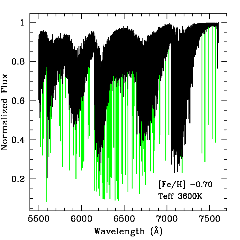
Figure 10: A synthetic spectrum from 5500-7600Å for the M giant with T_eff=3600K, in the core of 47 Tuc, including 5.4 million TiO lines, and Fe lines measured for the EW analysis of the IL spectrum. The green color indicates the synthesis performed with TiO plus Fe lines, and the black color indicates synthesis of TiO only. The TiO band heads of the alpha system are clearly visible.

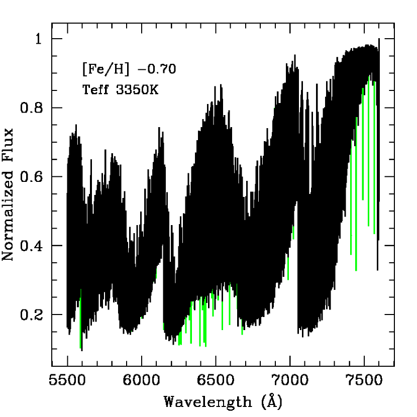
Figure 11: A synthetic spectrum from 5500-7600Å for the M giant with T_eff=3350K, in the core of 47 Tuc, including 5.4 million TiO lines, and Fe lines measured for the EW analysis of the IL spectrum. Colors are the same as for Figure 10. Notice the heavy TiO blanketing below $\sim$7300Å , that depresses the continuum and obliterates most atomic lines; the M giant window in the interval 7300–7600Å is relatively unaffected by TiO blanketing .

To understand the effect on the cluster core IL spectrum caused by blanketing and blending in the M star spectra, we present Figures 10 and 11, which show synthetic spectra in the region 5500–7600Å for the two M giants known to be in the core of 47 Tuc. The atomic lines measured in our IL EW spectrum analysis are also included in these figures. The synthetic spectra were computed using the 2004 version of the synthesis program MOOG (modified to take large line lists) and 5.4 million TiO lines from the 2006 version of the list by Plez (1998). We have not included other molecules or atomic lines in our calculations other than the list of Fe lines that were measured in the IL spectrum. We employed Kurucz alpha-enhanced model atmospheres with [Fe/H]=$-$0.70 dex and [O/Fe] and [Ti/Fe] = $+$0.3 dex. The model atmospheres were derived from the alpha-enhanced Kurucz grid; the cooler M giant model was extrapolated using a cubic spline technique, whereas the warmer M giant model was obtained by linear interpolation. Figures 10 and 11 show syntheses computed both with and without our Fe line list. The comparison demonstrates the effect of the TiO blends and pseudo continuum on the detectability of these atomic lines. Note that the TiO blanketing is significantly less than would be expected of solar-metallicity M stars of the same temperature (see Houdashelt et al. 2000) due to reduced TiO formation at the low metallicity of 47 Tuc.

It is clear from these figures that the TiO blanketing in the coolest of the 47 Tuc core M giants has severely attenuated the apparent continuum flux, and obliterated many of the atomic lines below 7300Å. Thus, pseudo equivalent widths for many of the atomic lines may be very small, suggesting that the coolest M star in the core of 47 Tuc probably makes very little contribution to the integrated-light EW of lines below 7300Å. The warmer of the two M giants in the core of 47 Tuc, with intermediate strength TiO bands, has greater optical flux and potentially a more serious effect on IL line EWs. Because TiO formation and the M giant fraction increases with metallicity, the EW abundance method used here will be less reliable for GCs more metal-rich than 47 Tuc.

The effect of the M giants on the integrated light EW of Fe I lines is difficult to assess without detailed computations due to two competing effects: First, while the neutral metal line strength increase for cooler stars, so does the TiO line blanketing, which effectively reduces the apparent continuum flux level. As indicated above, the continuum line blanketing is dominant for the coolest M giants. Second, the M giants constitute $\sim$8.0% of the total I band light, but only $\sim$2.5% of the total V band light for the cluster. Thus, the inclusion of the M giants would seem to be important for lines in the I band $\sim$8000–9000Å, but much less important in the V band, near 5500Å.

To test the effect of the M stars on our abundance results, we made two changes to the analysis described so far based on the HST photometry. First, we reduced the number of K giants by two and, second, we included the two M giant LPVs indicated by Lebzelter & Wood (2005). In order to include the M stars in the EW IL abundance analysis, we generated pseudo continuum fluxes and pseudo EWs for the two known 47 Tuc core M giants over the 5500–7600Å region, based on the spectrum synthesis calculations that we generated for Figures 10 and 11. As mentioned earlier, the syntheses included the Fe lines for which we had EW measurements, plus the 5.4 million TiO lines. The abundance input for the synthesis of each M giant was scaled to [Fe/H]=$-$0.70 dex, with [Ti/Fe] and [O/Fe]=$+$0.3 dex. The pseudo continuum flux levels were determined for the synthetic spectrum by integrating the theoretical spectrum synthesis flux over the wavelength bounds of the actual continuum windows used for measuring the EWs from the IL spectrum. For each iron line we averaged the synthetic fluxes in the adjacent continuum windows and then we calculated a pseudo EW by integrating the synthetic flux over 0.4Å, centered on the line. In most cases the pseudo EWs were smaller than if there had been no TiO, due to the pseudo continuum TiO blanketing, but in a few cases TiO features increased the apparent line EW. For yet other lines the pseudo EWs were negative, due to heavy blanketing in the continuum regions, but not in the lines. The ILABUNDS program was then enhanced to permit the use of pre-calculated pseudo EWs for the M giants to be included in the calculation of the total mean integrated-light EW.

To test the reliability of the calculations, we substituted pre-computed pseudo-EWs for a cmd box containing three K giants; the method reproduced the mean [Fe/H] within 0.006 dex of the mean determined without the approximation. In the nominal method, omission of the three K giants would have altered the derived mean iron abundance by 0.06 dex; thus, the approximation was accurate to about 10%.

When we compare the IL abundance results from the cmd with the two M-giants to abundances determined for a cmd in which the two M giants were excluded, the [Fe/H] from neutral and ionized species increased by 0.02 and 0.01 dex respectively. Furthermore, there was no obvious effect on the Fe lines redder than 7000Å, so the small discrepancy between lines redder and bluer than this wavelength does not appear to have been due to the M giants. Most likely the problem resulted from difficulties associated with extraction of the data for orders that are very close together on the CCD. With corrections of only 0.01 to 0.02 dex we can conclude that for 47 Tuc we are fortunate that the M giants in the cmd, with their heavy TiO blanketing, make a negligible difference to the derived abundances and the IL spectrum.

We note also that wavelength interval 7300–7600Å has vastly lower TiO opacity than surrounding regions, as can be readily seen in Figures 10 and 11. This window has been used for abundance analysis of individual M giants (e.g. Smith & Lambert 1985). Because the M giant continuum flux is unimpeded by TiO absorption in this window, a comparison of EW abundance results from lines in this region with line abundances from bluer wavelengths (where the continuum is heavily blanketed in M giants) will be sensitive to the M giant fraction in the cluster. The M giant window not only provides a potential probe for unresolved GC M giants, but the EW abundance method could be employed more reliably in this wavelength interval for metal-rich GCs, without the need to account for TiO blanketing effects. This is not a good option in our du Pont data, because there is some evidence that the orders might suffer from background subtraction problems at these wavelengths.

Because globular clusters more metal-rich than 47 Tuc have a larger fraction of M giants, they would require bigger corrections to the EW analysis result than the 0.01–0.02 dex found for 47 Tuc. For clusters with significant M giant populations, and very large abundance corrections to the EW technique (using pseudo EWs), it will be necessary to abandon the EW analysis technique entirely, and instead use spectrum synthesis profile matching for every line and continuum region not in the M giant window. This would significantly increase the effort required and the uncertainty of the results. Further computational studies are necessary to determine the metallicity beyond which it will be important to employ this spectrum synthesis profile matching abundance method.

In summary, we have explored the effect of the M giant population on the IL spectrum and abundance analysis for 47 Tuc using an approximate method of pseudo-EWs for these stars, including synthesis of millions of TiO lines. We find that the derived overall GC IL abundances change by only 0.02 to 0.01 dex for Fe I and Fe II lines respectively. Thus, the M giants could safely be ignored in an abundance analysis of 47 Tuc, but for higher metallicity GCs, with a larger fraction of M stars, the effect will be greater, possibly enough to require use of a laborious, and less reliable, synthesis profile matching abundance technique. For GC IL abundance studies at high metallicities, the M giant window at 7300–7600Å would constitute a valuable check on the abundance results from lines outside this window.

3.2.3 Abundances of Elements Other than Iron

Abundances for elements other than Fe were computed using the EWs and atomic parameters listed in Table 2. Due to the velocity broadening in 47 Tuc, various lines that are normally clean in red giant stars were not usable. A notable example is the strongest line of a Mg I triplet at 6318.708Å, which is blended with a Ca I line 0.1 Å to the blue. The [O I] line near 6300Å is another unfortunate case, as it is blended with the very strong telluric emission line. In GCs with large systemic velocities, however, the oxygen feature may be usable.

Elements with odd numbers of protons or neutrons, or elements with significant fraction of odd-numbered isotopes, suffer from hyperfine splitting (hfs) of the energy levels. For lines with large hfs splittings, the line is split into many non-overlapping, or partially overlapping, sub-components that reduce or eliminate saturation of the feature. Desaturation by hfs can significantly lower the computed abundance compared to a single line. However, for the case of unsaturated, weak, lines (e.g. $\leq$20–30mÅ), the hfs treatment gives the same result as a single line approximation.

We have computed hfs abundances for lines of Ba, Co, Cu, Eu, La, Mn, Nd, V and Zr, by synthesis of each line including all hfs components. Previous experience with lines of Al, Na, Sc and Y indicated that the hfs effect is too small to make a difference, so we neglected to perform hfs abundance calculations for those species. The A and B hfs constants for each line were taken from references indicated by McWilliam & Rich (1994) and McWilliam et al. (1995), and the wavelengths and strengths of the hfs components were computed using standard formulae. For the lines considered here we find typical hfs abundance corrections for Cu, Co, Mn, La, V and Nd of $-$0.8, $-$0.3, $-$0.3, $-$0.15, $-$0.1 and $-$0.08 dex respectively; abundances derived with hfs are always lower than abundances derived assuming a single line. We note that for the La II line at 6774Å hfs constants were available only for one level in the transition; however, we are still able to use the line because its small equivalent width ensured that the single line treatment was reliable.

In Table 4 we list the average integrated-light abundances for all measured elements in 47 Tuc. For abundance ratios relative to Fe we employed the solar abundance distribution of Asplund et al. (2005), except for Fe, for which we adopted a solar abundance of 7.50 dex. Table 4 also contains comparisons with other analyses for 47 Tuc: Brown & Wallerstein (1992), Carretta et al. (2004), Alves-Brito et al. (2005), Wylie et al. (2006), and Koch & McWilliam (2008).

A difficulty in the comparison with previous studies is that there is variance between the earlier works in the 0.1 to 0.2 dex range. This not surprising, given the variety of techniques and assumptions employed by previous studies to measure chemical abundances for 47 Tuc. If we compare our mean abundance ratios with the mean of the previously published studies listed in Table 4, we find that, of 14 species measured by two or more previous studies, our values are higher by 0.08 dex with a standard deviation of 0.17 dex. Only two [X/Fe] ratios measured here differ by more than two sigma from the mean literature values: Zr and Eu. These elements are represented by one weak line each. In the case of Zr the line occurs at the ends of two adjacent orders, where the noise is large. However, since our [Zr/Fe] ratio, near zero, is similar to our other heavy elements it seems possible that the value found here is correct. The single Eu II line in our spectrum, at 6645Å , is quite weak (EW$\sim$16 mÅ), so it is possible that our EW is artificially low due to noise.

It is notable that our [Na/Fe] ratio, at $+$0.45 dex, is larger than the mean of previous studies by 0.2–0.3 dex, depending on whether the Wylie et al. (2006, henceforth W06) result is included. This difference may not be significant, given the 0.17 dex rms scatter in our Na abundances, however part of the difference likely results from the low solar photospheric abundance for Na given by Asplund et al. (2005), which is 0.10 dex lower than their meteoritic value (itself lower by 0.06 dex than earlier estimates of the solar meteoritic Na abundance). Yet another possibility is that the integrated-light Na abundance may really be higher than in individual red giant and turnoff stars if a significant fraction of the AGB star population in 47 Tuc shows proton burning products in their atmospheres. In this regard it is interesting that the sample of W06 is dominated by AGB stars and is unusually enhanced in Na, with a mean [Na/Fe]=$+$0.65 dex. If our high Na values reflect proton burning products in the envelopes of luminous evolved stars in the cluster, then we might also expect to see depletions of O, and possibly Mg, combined with enhancements of Al in the integrated-light analysis. We were unable to measure O in this work, however we do find that Mg is lower than the average of the published studies by 0.18 dex, and Al is higher by 0.15 dex. More detailed work would be required to investigate this possibility.

Besides these comparisons with other studies of 47 Tuc we may investigate how well our integrated-light abundances compare with the composition of the Galaxy in general. This is particularly useful for elements studied here that were not included in previous work on 47 Tuc (e.g. Cu, Mn). We are interested to know whether our integrated-light abundances are consistent with Galactic stars and clusters with metallicity similar to 47 Tuc. For example, the mean [X/Fe] for alpha elements studied here (Mg, Si, Ca, Ti), at $+$0.34 dex, compares well with the halo average of $+$0.35 (e.g. see McWilliam 1997).

As discussed above the [Na/Fe] and [Al/Fe] ratios are higher (by $\sim$0.2 and 0.1 dex respectively) than typically seen for the 47 Tuc metallicity, but this is likely due to proton burning products in the atmospheres of the most luminous stars in the cluster. Within the measurement uncertainties our 47 Tuc [Mn/Fe] ratio, at $-$0.44 dex, is lower than, but consistent with, the deficient values seen in Galactic stars and clusters at the same [Fe/H], near $\sim$$-$0.3 dex (e.g. Sobeck et al. 2006; Johnson 2002; McWilliam, Rich & Smecker Hane 2003; Carretta et al. (2004).

In the disk and halo of the Galaxy the [Cu/Fe] ratio declines roughly linearly with decreasing [Fe/H], reaching a value of $\sim$$-$0.6 to $-$0.7 dex by [Fe/H]$\sim$$-$1.5 (Mishenina et al. 2002; Simmerer et al. 2003). At the metallicity of 47 Tuc previous studies indicate [Cu/Fe] near $-$0.1 to $-$0.2 dex. This is entirely consistent with the [Cu/Fe] ratio found here, at $-$0.13 dex, from our integrated-light analysis.

W06 abundances for the light s-process elements Y and Zr are enhanced by $\sim$0.6 to 0.7 dex, in contrast to the solar-like ratios found here; unfortunately, there is insufficient data from other studies of 47 Tuc to draw a conclusion regarding these two elements. W06 selected a sample of AGB and RGB stars from 47 Tuc, so it may be that their s-process abundance enhancements simply reflect AGB evolution of the stars themselves; however, they found similar s-process enhancements in both their RGB and AGB populations. Previous studies of Y and Zr in nearby Galactic disk and halo stars (e.g. Edvardsson et al. 1993; Gratton & Sneden 1994) show that [Y/Fe] remains at the solar ratio to the metallicity of 47 Tuc, and that [Zr/Fe] is very slightly enhanced, near 0.1 to 0.2 dex, consistent with the results for these two elements found here. We suggest that the enhancements found for Y and Zr by W06 are most likely due to either systematic errors, or result from s-process enhancements in their AGB stars.

The [Eu/Fe] ratio in Galactic metal-poor stars follows a trend similar to the alpha elements, increasing with decreasing [Fe/H] in the solar neighborhood, to a value near 0.3 to 0.4 dex and roughly flat below [Fe/H]$\sim$$-$1 (McWilliam & Rich 1994; Woolf et al. 1995). At the 47 Tuc metallicity the measured [Eu/Fe] ratio of Galactic stars ranges from 0.2 to 0.3 dex. Thus, our rather low [Eu/Fe] ratio, at 0.04 dex, is not only lower than other reported measurements in individual 47 Tuc stars, but is also at odds with the general trend seen in Galactic stars in general. With a central line depth of only $\sim$3 percent it is hardly surprising that the Eu II line at 6645Å gives discordant results.

Table 4 indicates a 0.25 dex enhancement in [Sc II/Fe], based on one line, but a normal solar-scaled Sc abundance from a single Sc I line. However, the Sc II enhancement in our integrated-light analysis is in qualitative agreement with claims of mild Sc enhancements with decreasing metallicity (e.g. Bai et al. 2004; Nissen et al. 2000); but see Prochaska & McWilliam (2000).

The remaining elements roughly scale with [Fe/H], similar to the trends seen in the Galaxy (e.g. Edvardsson et al 1993; Sneden & Gratton 1994; McWilliam 1997).

The above abundance trends indicate that our integrated-light 47 Tuc abundances are consistent with the composition of Galactic stars of similar metallicity. This supports the idea that we have successfully managed to perform detailed chemical abundance analysis on the integrated light spectrum of the core of 47 Tuc, using the observed color-magnitude diagram as an essential input ingredient.

3.3 Integrated-Light Abundance Analysis With Theoretical Isochrones

For GCs beyond the Local Group it is not currently possible to resolve individual stars to obtain empirical cmds. Thus, the next step in developing an IL abundance analysis strategy for extra-galactic clusters is to use theoretical isochrones with parameters constrained by the IL spectrum. In this paper, we have employed theoretical isochrones from two groups: Padova and Teramo. The Padova isochrones of Girardi et al. (2000) and Salasnich et al. (2000) were obtained from the group’s website. The isochrones we use are the set computed with convective overshoot and a constant mixing length. For the Padova isochrones, our IL abundance calculations were made with scaled solar composition only, due to the very limited selection of alpha-enriched models. The competing isochrones from the Teramo group (e.g. Cassisi, Salaris & Irwin 2003; Pietrinferni et al. 2006) were available for a variety of assumptions at the start of our work, including alpha-enhanced or scaled solar composition, with or without convective overshooting, two mass-loss rates (Riemer’s mass-loss parameter $\eta$=0.2 and 0.4), and normal or extended AGB. Maraston (2005) investigated the merits of the these various Teramo isochrones, as well as those from the Padova group, by comparing to observed clusters and favored the Teramo (BaSTI) isochrones. Guided by the Maraston (2005) and the BaSTI web site recommendations, we selected the Teramo classical evolutionary tracks with no overshooting for the treatment of the core, a metallicity-dependent mixing length parameter, an extended AGB, and a mass-loss parameter of $\eta$=0.40. Most recently the Teramo isochrones have been updated for corrections to the alpha-enhanced opacities initiated by Ferguson et al. (2005). While the Teramo isochrones offer a greater parameter flexibility than the Padova isochrones, we believe that it is useful to compare the IL abundance results obtained using both the Teramo and Padova isochrones.

Both the Teramo and Padova isochrones are provided without luminosity or mass functions. We therefore computed the frequency of each point on the theoretical isochrones using the IMF recommended by Kroupa (2002), and the initial masses indicated for each isochrone point. A simple program was used to bin points along the theoretical isochrones into cmd boxes, each containing at least 3.5% of the total V-band flux. For each box the V-band flux-weighted model atmosphere parameters were computed according to the equations 4, 5 and 6, above. In this way, the theoretical isochrones provided an input file of atmosphere parameters for our IL abundance analysis program with 21–27 cmd boxes, similar to the input file used for the observed cmd analysis (see Table 3).

For the most luminous stars in the cluster, near the tip of the giant branch, small number statistics can lead to incomplete sampling if the cluster has a low total luminosity or if only a small fraction of the cluster is scanned with the spectrograph. The latter is true for our spectrum of 47 Tuc. In order to address the issue of this statistical incompleteness in the observed IL spectrum of the 47 Tuc core we used the theoretical isochrones and Kroupa IMF to estimate the number of stars in each cmd box. To make this calculation it was necessary to input an estimated M_v for the 32$\times$32 arc second region of the core scanned with the spectrograph slit. We did this by summing the observed V-band fluxes of the stars in the HST core photometry and correcting for our adopted distance modulus and foreground reddening. This procedure resulted in a value of M_v(core) =$-$6.25. As the giant branch tip is approached, the number of stars in the high luminosity cmd boxes decreases. We truncated the top of the cmd luminosity function at the point where the integrated probability of finding a single star fell below 0.5, since it was more probable that no stars were present in the cluster beyond this point.

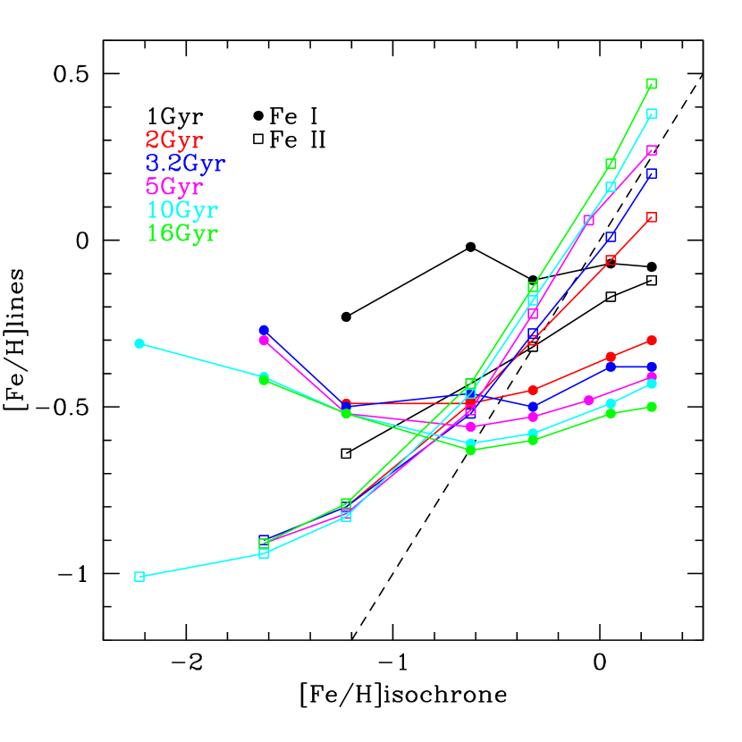
Figure 12: Computed abundances from Fe I and Fe II lines in 47 Tuc (filled circles and open squares respectively) for Padova isochrones of various ages and metallicities. Note the different sensitivity to isochrone metallicity of the Fe I and Fe II lines, and the dependence on age. The dashed line is the locus of [Fe/H] from the Fe lines equal to the value in the input isochrone.

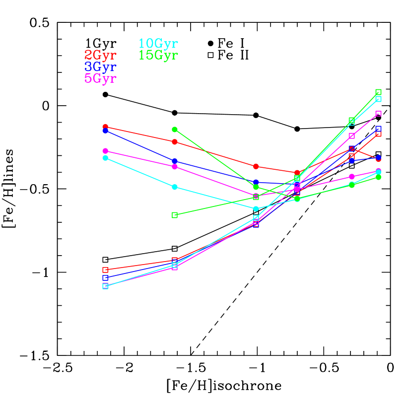
Figure 13: Computed abundances, from Fe I and Fe II lines (filled circles and open squares respectively) in 47 Tuc, for various ages and metallicities, using Teramo (BaSTI) alpha-enhanced, AGB-enhanced, classical isochrones with mass loss parameter $\eta$=0.40. Note the different sensitivity to isochrone metallicity of the Fe I and Fe II lines, and the dependence on age.

Following the same analysis procedures as before we computed Fe I and Fe II abundances from the 47 Tuc IL EWs using theoretical isochrones, from the Padova and Teramo groups, in place of the observed cmds. However, because the age and metallicity were not known in advance we computed the line abundances for a range of assumed age and metallicity. For the Padova scaled solar isochrones we used scaled solar composition Kurucz model atmospheres with the ODFNEW opacity distribution function; the results are presented in Figure 12. From the Teramo (BaSTI) group, we used the alpha-enhanced isochrones throughout, corrected for the Ferguson et al. (2005) alpha opacities, together with the alpha-enhanced Kurucz stellar model atmosphere grid with the AODFNEW opacity distribution functions (Castelli & Kurucz 2004). For the Teramo (BaSTI) isochrones, spanning a large range of age and metallicity, the iron abundance results are shown in Figure 13.

In Figure 12 and 13, the Fe I abundances that we identify using the isochrones at any given age change by less than 0.2 dex over the whole range of input isochrone metallicities. The Fe I abundances agree with the input isochrone metallicity near [Fe/H]$\sim$$-$0.5 to $-$0.6 dex for the 15 Gyr models. The figures show that significantly higher [Fe/H] values are obtained from the lines if very young ages are adopted; at 1Gyr, agreement between isochrone metallicity and line abundances occurs near $-$0.1 dex, while for old ages the result hardly changes at all between 10 and 15 Gyr. For iron abundance uncertainties of $\sim$0.1 dex the convergence of the stellar isochrones result in an insensitivity to age older than about 5 Gyr.

The Fe II line abundances in Figures 12 and 13 increase much more strongly with isochrone metallicity than the Fe I lines. We interpret the strong dependence of the Fe II abundance with adopted input isochrone metallicity as follows: when the adopted isochrone metallicity is overestimated, the computed continuum opacity is artificially enhanced due to increased H^- from increased electrons from the ionization of the extra metals. In this case, to match the integrated-light Fe II line strength requires an over-estimate of the true metal content, as this depends on the line to continuum opacity. In this way, the computed Fe II abundances increase with the adopted isochrone Z. For Fe I lines, on the other hand, an overestimated isochrone metallicity results in enhanced recombination of Fe II to Fe I in the model atmospheres. This increase in the Fe I number is matched by a similar increase in the H^- opacity and, as a result, the computed Fe I line strengths remain relatively unchanged for a given input isochrone metallicity. At very low isochrone Z, around 1/100 solar, the Fe II abundance trends in Figures 12 and 13 become less sensitive to metallicity. We believe that this results from the fact that the electron density in very metal-poor stellar atmospheres no longer depends upon ionization of metals, but is dominated by the ionization of hydrogen. We note that the Fe II abundances in Figures 12 and 13 also show a sensitivity to isochrone age, with the largest change for the youngest ages; but the direction of the derived abundance changes is such that younger isochrones give lower Fe II abundances, whereas Fe I abundances are increased.

It must be noted that the initial impression from Figures 12 and 13 is that the self consistency appears to be better for the Padova iron abundance than for the Teramo results, because the Fe II and Fe I abundances and the isochrone [Fe/H] value agree at similar values, near $-$0.6 dex as mentioned above. On the other hand, in these figures, the Fe I and Fe II agreement for the Teramo-based analysis agree at much lower [Fe/H] than Fe I and the isochrone [Fe/H]. This could easily be due to higher adopted [$\alpha$/Fe] ratios for the Teramo isochrones and Kurucz alpha-enhanced models than actually present in 47 Tuc. Furthermore, the whole issue is somewhat confused by the recent changes in the solar composition by Asplund et al. (2005) and the delay between such solar results and the compositions used to compute stellar model atmospheres and isochrones. While the Padova agreement is better we must remember that 47 Tuc really is enhanced in alpha elements (e.g. see Table 4), as expected from its overall metallicity, so alpha-enhanced models are appropriate. Thus, it may be that the Fe I, Fe II and isochrone [Fe/H] agreement found by use of the solar-composition Padova isochrones was simply fortuitous.

3.3.1 Isochrone Problems?

In order to identify the cause of the differences between the iron abundance results from observed cmd and theoretical isochrones, we have compared the observed and predicted luminosity functions for 47 Tuc in detail. To do so, we adopt the 47 Tuc distance modulus of 13.50$\pm$0.08 and age, of 11.2$\pm$1.1 Gyr, from Gratton et al. (2003). We note that more recent results reviewed by Koch & McWilliam (2008) indicate a mean distance modulus of 13.22, but this short scale leads to a change in $\log{g}$ of $\sim$0.1 dex, and does not significantly affect the resultant abundances. For the reddening we averaged the two E(B$-$V) values given by Gratton et al. (2003), at 0.021 and 0.035, with the value of 0.032 from Schlegel et al. (1998), for a mean of 0.03 magnitudes. For this comparison, we adopted the alpha-enhanced, AGB-enhanced, Teramo isochrones with a metallicity of Z=0.0080 (corresponding to [Fe/H]=$-$0.70 according to the Teramo web site), and a mass-loss parameter of $\eta$=0.40. We note that the assumed conversion between [Fe/H] and Z for alpha-enhanced composition varies significantly in the literature; this is likely due to the recent changes to the best estimates for the solar oxygen and iron abundances (e.g. Asplund et al. 2005).

In Figure 14, we compare the observed and theoretical V-band luminosity functions for 47 Tuc. We note that while the adopted age of 11 Gyr provides a good match to the cmd at the main sequence turnoff and the Red Clump, it is also possible to obtain good matches with the observed luminosity function using older ages and a shorter distance modulus for the cluster. For this reason, we cannot confidently measure the cluster age. For the isochrones which produce good matches to the observed luminosity function, three major differences are still apparent: a deficit of stars below the turnoff in the observations; a general excess of observed giants above the Red Clump, highlighted by the spike in stars at the AGB bump; and an excess in the observed cmd at the very tip of the giant branch.

While it might be reasonable to assume that the paucity of stars observed below the main sequence turnoff is due to incomplete photometry, Howell et al. (2000) has noted this in the data and attributed it to a real deficit of low-mass stars, presumably caused by dynamical mass-segregation processes. Mass segregation was first observed in the 47 Tuc core by Paresce et al. (1995) and is known in numerous other cluster cores (e.g. King, Sosin & Cool 1995; Ferraro et al. 1997; Gouliermis et al. 2004). The striking excess of AGB bump stars in the observed core V-band luminosity function corresponds to the group of stars near V$\sim$13.2 and (B$-$V)$\sim$1.0 in the cmd shown in Figure 5. We note that this same group of stars is present in the Kaluzny (1997) V,V$-$I 47 Tuc color-magnitude diagram of an outer field. We investigated a number of parameters for the Teramo isochrones, but we could find no combination of ages, from 10 to 14 Gyr, or mass-loss rate that gave a spike corresponding to the AGB bump. We conclude that the models are deficient in predicting the AGB bump, despite the use of “AGB enhanced” models. This under-prediction is reminiscent of the Schiavon et al. (2002) 0.4 dex deficiency of the theoretical AGB numbers compared with observations; however, here we require an enhancement for the AGB bump only. Finally, while there is an excess of flux at the tip of the observed giant branch luminosity function, compared to the predictions, the total flux at the tip comes from only 5 stars; thus, at $\sim$30% this flux excess is within the 1$\sigma$ Poisson noise of $\sim$45%. Therefore, while the excess flux from the giant branch tip is real, it does not indicate a problem with the theoretical isochrone.

We have applied two corrections to the theoretical Teramo isochrone to make the corresponding V-band luminosity function appear more like the observed function. First, to approximately match the main sequence turnoff region, we ignore all stars with M_v more than $+$4.90. Second, to match the observed AGB bump region, we apply an enhancement factor of 3.0 to stars in the M_v range from $-$0.10 to $-$0.70. Figure 15 compares the observed luminosity function with the corrected Teramo isochrone; the match is significantly improved, although it is clear that the real cluster still has slightly more flux coming from the giants than the model. Although not plotted here, we note that the theoretical luminosity function for Padova isochrones with age and abundance parameters like 47 Tuc show differences with the 47 Tuc luminosity function that are very similar to those discussed above; they also show a deficit in the predicted AGB bump by a factor of 3, and RGB tip deficit slightly more than for the Teramo isochrones, and a near-identical overestimate of dwarf stars below the turnoff.

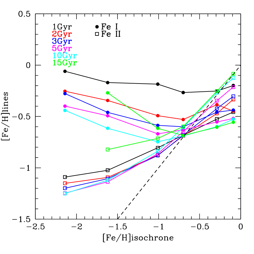
Figure 16: Computed abundances for Fe I and Fe II (filled circles and open squares respectively) in 47 Tuc integrated light, using Teramo (BaSTI) isochrones with corrections of $-$0.125 and $-$0.165 dex respectively; similar to Figure 13. Note that for 10 and 15 Gyr Fe I and Fe II abundances are equal $\sim$0.3 dex lower than the isochrone metallicity; we do not understand this inconsistency.

A computation of the IL abundances from the measured Fe I and Fe II lines gives different results for the original 47 Tuc Teramo isochrone and our modified version of the isochrone with the MS and AGB bump corrections. For our list of Fe I lines the mean difference is $-$0.125 dex, while for the Fe II lines the difference is $-$0.165 dex, where these differences are corrected-isochrone minus uncorrected-isochrone abundance. To first order the differences provide zero-point offsets to be applied to uncorrected-isochrone abundances. We note that these offsets are valid only for one specific age and metallicity. Given the variability of turnoff, RGB, HB and AGB stars in GCs with different ages and metallicities it is unlikely that these offsets will be universal. When these corrections are applied to the abundances in Figure 13 we obtain a corrected plot, Figure 16, showing the dependence of [Fe I/H] and [Fe II/H] on assumed age and isochrone metallicity. We note that there is a systematic trend of decreasing derived Fe I abundance with increasing age, similar to the Padova isochrone results in Figure 12, but at 15 Gyr the Fe I abundances show an increase over the 10 Gyr model; a similar turn-around occurs in the direction of the derived Fe II abundances. This effect appears to result from a change in the core helium-burning stars in the isochrone from red clump to blue horizontal branch, and is related to age, metallicity and the mass-loss parameter, $\eta$.

As shown in Figure 16, the Fe I lines give $-$0.70 dex for the 10–15 Gyrs isochrones with [Fe/H] $-$0.70 dex. The satisfying agreement between isochrone [Fe/H] and the value derived from Fe I lines indicates an older age range (10–15 Gyr) for 47 Tuc, as expected from color-magnitude diagrams (e.g. Gratton et al. 2003); ages of 3 Gyr or less are completely inconsistent with the Fe I line abundances. The Fe II lines give higher abundances than by 0.08 and 0.09 dex, respectively, for the 10-15 Gyr isochrones with [Fe/H]=$-$0.70 dex. While the difference of $\sim$0.08 dex between Fe I and Fe II abundances are within measurement uncertainties, there is a systematic difference which bears some thought. We suggest three possibilities that might explain these systematically higher Fe II abundances derived from the theoretical isochrones. First, there may be systematic errors in the measured equivalent widths of Fe II lines, which are weak and often blended in the 47 Tuc IL spectrum. Second, the alpha enhancement adopted for the theoretical isochrone may be higher than the actual alpha enhancement of the cluster. This may be related to the reduction in the solar oxygen abundance by Asplund et al. (2005). Third, there may be a statistical variance, or other mechanism, that increased the representation of stars at the tip of the giant branch in excess of those predicted by the Teramo isochrones.

Given that our Padova isochrones employed solar composition rather than including the alpha enhancements necessary for to 47 Tuc, more detailed comparisons of the merits of the two sets of theoretical isochrones is not possible at this time.

3.3.2 Isochrone Diagnostics and Abundances for Unresolved GCs

A significant difficulty in the use of the theoretical isochrones for IL abundance analysis is the choice of isochrone parameters of age, metallicity, and alpha enhancement. Fortunately, for 47 Tuc we can assume a roughly old age, and be assured that our Fe I abundances will be close to the truth. For unresolved clusters, the integrated colors could be used to constrain the combined effects of age and metallicity; however, the well-known age-metallicity degeneracy seen in cluster cmds makes determination of the isochrone parameters impossible solely on the basis of photometry. This is similar to the covariance between temperature and metallicity in the abundance analysis of individual stars. For full spectroscopic analysis of individual stars, various abundance diagnostics are used to constrain the atmosphere parameters. Likewise, we propose to use diagnostic spectral features to constrain the GC isochrone parameters, resulting in an isochrone choice that is completely consistent with the spectra. The most obvious example of such a diagnostic is that the isochrone metallicity must be consistent with the abundances computed from the absorption lines; this may include the alpha enhancement, which should agree with the abundances returned from the alpha element lines. We discuss a variety of other diagnostics below.

In general the abundance computed for an individual line depends on the isochrone age and metallicity, but also on the excitation potential and ionization stage of the line. For example, if an isochrone with an incorrect age is adopted in the analysis, abundances derived from low excitation Fe I lines will be different than for high excitation Fe I lines due to the inappropriate stellar temperatures, resulting in a non-zero slope in the plot of iron abundance versus excitation potential. Our work (see below) bears out this expectation, however we also note that this use of excitation potential versus iron Fe I line abundances as an age diagnostic may be complicated by the presence of a hot horizontal branch that might be confused with hot main sequence stars in old, low metallicity clusters. The Fe II lines should also provide a diagnostic, because they are sensitive to the electron density (unlike the Fe I lines), which in individual stars is a strong function of gravity. Thus, a constraint on the isochrone parameters comes from the consistency of the abundance results for lines from both ionization stages of iron.

Another potential spectral diagnostic is derived from the computed abundance of individual Fe lines as a function of wavelength. A sub-population of relatively hot stars within a cluster will have its greatest contribution to the total flux at blue wavelengths. Thus, we may only expect agreement between iron abundances from blue and red wavelengths with the correct mix of hot and cool stars. This constraint of consistency with wavelength is similar to the the method used by Maraston et al. (2006), who found that thermally pulsing AGB stars contribute significantly to the total infrared fluxes of stellar populations in the $\sim$1 Gyr age range.

To investigate spectral diagnostics of the isochrone parameters we begin with Figure 17, which shows iron abundances versus EW and excitation potential (EP) for the lines in Table 2. Abundances for this plot were derived using a theoretical, alpha-enhanced, Teramo cmd for an age of 15 Gyr. Similar plots are used as diagnostics for studies of individual stars. Figure 17 shows that the iron abundance is approximately independent of EW and EP, which indicates that the microturbulent velocities and temperatures employed in the abundance calculations were consistent with the measured line EWs.

Figure 18 shows the results of our abundance calculations using a Teramo isochrone for an age of only 1Gyr. In this case the plot of iron abundance versus EW indicates that abundances derived from strong and weak lines do not agree, with strong lines giving higher abundances. In an analysis of a single star’s spectrum, this observation would indicate that the adopted microturbulent velocity parameter is too small. Since Figures 6 and our analysis using the empirical cmd has already demonstrated that our adopted microturbulent velocity law is roughly correct, the disagreement between strong and weak lines in Figure 18 suggests that the input isochrone has too many stars with low microturbulent velocity. This suggests that the input isochrone contains more dwarf stars than the cluster, because dwarf stars have lower microturbulent velocities than giants. The plot of iron abundance with excitation potential for the 1 Gyr isochrone shows a decrease in abundance with increasing EP. For single stars this would indicate that the adopted temperature is too low. In the integrated light analysis this suggests that there is an excess of hot stars in the input isochrone compared to the real cluster, which is consistent with the idea that there is a larger fraction of dwarf stars in the 1Gyr isochrone than in the observed cluster. Thus, both the EW and EP plots suggest that the older, 10–15 Gyr isochrones provide better consistency among computed iron line abundances than do very young isochrones ($\sim$1 Gyr).

Figures 17 and 18 are used here only to demonstrate diagnostic possibilities; clearly careful measurement of the deviations from zero slope in the EW and EP plots offers the possibility to determine the best fit isochrone age. The measured 1$\sigma$ uncertainty in the slopes of these two figures, at 0.00063 dex/mÅ and 0.019 dex/eV, respectively, is sufficient to provide 3$\sigma$ constraints on ages younger than 2 Gyr only. However, a factor of 2 improvement in the abundance measurement uncertainties would permit 3$\sigma$ measurement of ages up to 5 Gyr. This reduced abundance scatter could reasonably be expected by mitigation of uncertainties due to $gf$ values, blends, and use of higher S/N spectra. In this regard a differential abundance technique, relative to a standard giant or a known cluster, and a careful study of each line would be fruitful. Indeed, results with a GC training set (Bernstein et al. 2008) suggests that it will be possible to provide age constraints for the current plots to ages up to $\sim$3–5 Gyr. Older than 5 Gyr the abundance slope differences are too small to constrain the age.

In principle, iron ionization equilibrium (consistency of the Fe I and Fe II abundances and isochrone metallicity) can also be used to constrain the isochrone age. This is particularly sensitive to the Fe II abundance, which requires the additional constraint of the isochrone alpha enhancement and proper accounting for the most luminous stars in the isochrone, since the Fe II lines are strongest at the lowest gravities. In Figure 16 we see that the 5 Gyr isochrone for our 47 Tuc model is closest to consistency of Fe I, Fe II abundances and the isochrone metallicity; however, the 47 Tuc cmd suggests a significantly older age, close to 12 Gyr (e.g. Koch & McWilliam 2008).

Another age diagnostic may be obtained from a plot of iron abundance with wavelength. In this case, excessively young ages would give different abundances for lines at blue wavelengths. In practice, both our 1Gyr and 10–15 Gyr give noisy, approximately flat, trends of abundance with wavelength for our spectra; although much bluer spectral lines may have shown sensitivity to age.

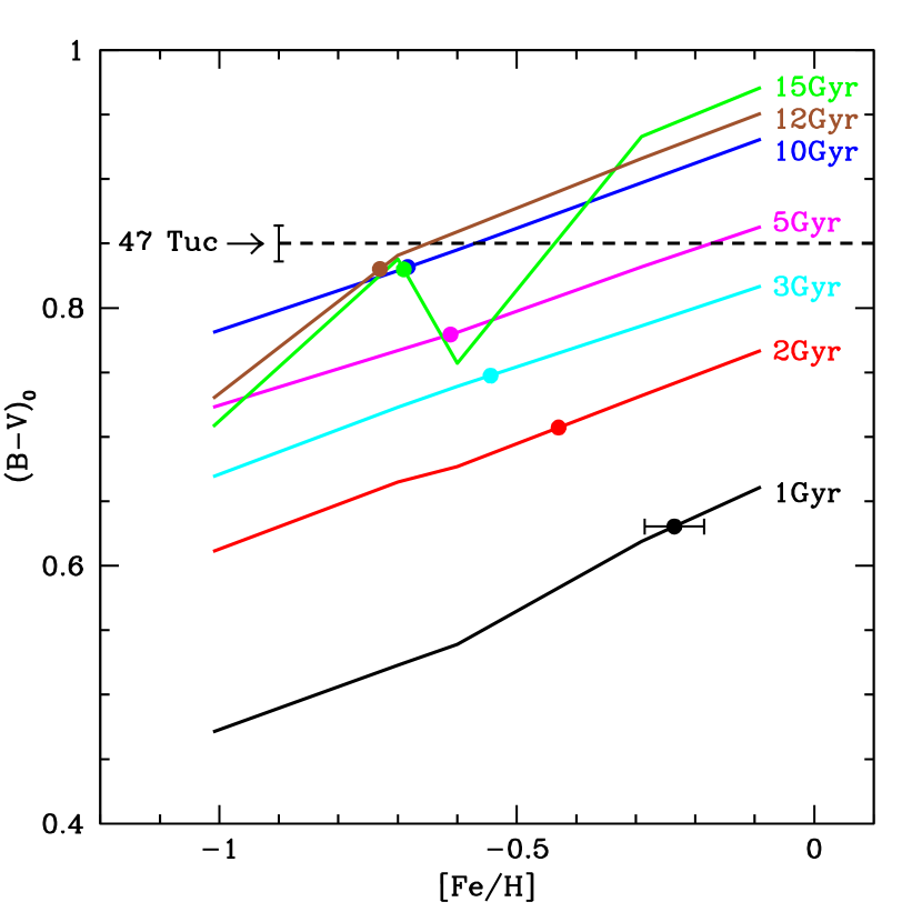
Figure 19: Solid lines indicate our computed integrated-light (B$-$V)₀ GC colors, based on Teramo isochrones (canonical alpha-enhanced models with $\eta$=0.4), for a range of age and [Fe/H]. Filled circles indicate the [Fe/H] values derived from 100 Fe I lines in the IL spectrum, depending on assumed age. The dashed horizontal line shows the observed (B$-$V)₀ color for the inner 47 Tuc region included in our IL spectrum, as measured by Peterson (1986). Error bars indicate $\pm$1$\sigma$ uncertainties in the observed color and on the mean [Fe/H]. The intersection of the observed (B$-$V)₀ color with derived [Fe/H] point indicates a self-consistent solution at [Fe/H]=$-$0.70$\pm$0.056 and age $\geq$10 Gyr. Note that the 15 Gyr isochrone color trend differs from younger isochrones, due to the presence of a blue horizontal branch at 15 Gyr, instead of a red clump.

Given the limitation associated with spectral age diagnostics we now include broad-band, B$-$V colors, combined with the abundances derived from the spectra, to improve constraints on both age and metallicity. Essentially we use the different sensitivity to age of the integrated-light colors and abundances derived from the Fe absorption lines to simultaneously constrain age and [Fe/H]. In Figure 19 we show theoretical integrated-light B$-$V colors, for alpha-enhanced, $\eta$=0.4, Teramo isochrones with ages ranging from 1 to 15 Gyr. To calculate the cluster B$-$V color we integrated the predicted B and V fluxes for each point on the Teramo isochrone, appropriately weighted by the Kroupa IMF. We note that our IL B$-$V colors depend upon the reliability of the Teramo isochrones, and as we have already seen the AGB bump in the Teramo predictions are under-estimated compared to the 47 Tuc cmd. Fortunately, when we enhance the AGB bump of the Teramo isochrones the effect on our IL B$-$V color is negligible, with a change of only $-$0.004 magnitudes; therefore, we should lower the loci in Figure 19 by 0.004 magnitudes. We note that the effect of $\alpha$-enhancement on the integrated B$-$V color seems to be rather small for 47 Tuc parameters: for 12 Gyr and [Fe/H]=$-$0.70 our solar composition calculations give B$-$V 0.012 magnitudes bluer than the alpha-enhanced isochrone; thus, an uncertainty of $\sim$0.1 dex in the adopted alpha-enhancement would change the predicted B$-$V color by only 0.002 magnitudes. Another isochrone morphology effect occurs for the oldest tracks with the choice of mass-loss parameter, $\eta$, such that the helium burning stars at high mass-loss and low masses reside on the Horizontal Branch instead of the Red Clump. Indeed, the unusual behavior of the 15 Gyr track in Figure 19 is due to the emergence of the Horizontal Branch compared to younger isochrones; notably, the 15 Gyr isochrone with a lower mass-loss rate ($\eta$=0.2) behaves more regularly. Another isochrone systematic that can affect the our colors is the relationship between color, temperature and metallicity adopted by the Teramo group: the B-band is particularly challenging for spectrum synthesis, due to the large number of strong absorption lines in red giants, and the M star spectra are especially complex.

Figure 19 indicates the computed [Fe/H] for each age track, where the isochrone metallicity and [Fe/H] from the Fe I lines are consistent, as derived from Figure 16. These points form a locus that intersects the observed B$-$V color for the isochrone whose age and metallicity are consistent with both the photometric and spectroscopic data. The horizontal dashed line in the figure shows the observed IL B$-$V color of 47 Tuc from Peterson (1986), de-reddened for E(B$-$V)=0.03; the $\pm$1$\sigma$ error bar of the observed (B$-$V)₀, at 0.014 mag., is the quadrature sum of 0.01 magnitude uncertainties in both the observed color and the reddening.

The random error on the mean integrated-light [Fe/H] value, determined from the Fe I lines is 0.021 dex. The systematic uncertainties, as discussed in section §3.2.1, give a total random + systematic uncertainty on the [Fe I/H] values in Figure 19, of 0.050 dex; this is indicated by the horizontal $\pm$1$\sigma$ error bars on the 1Gyr point. When we also include the 0.025 dex uncertainty, due to the choice of isochrone age (estimated from Figure 19), the total 1$\sigma$ systematic + random uncertainty on unresolved IL [Fe/H] from Fe I lines becomes $\pm$0.056 dex.

Other potential sources of uncertainty include non-LTE corrections, and errors in the input isochrones, including the adopted helium mass fraction, Y, the assumptions about mixing length, mass-loss and innumerable other parameters that went into the Teramo isochrone calculations.

Figure 19 constrains the 47 Tuc isochrone age in the range 10 to 15 Gyr, with [Fe/H]=$-$0.70 $\pm$0.056 dex. The B$-$V color and [Fe/H] uncertainties indicates that the 8 Gyr isochrone is ruled out at the 2.7$\sigma$ level. This integrated-light result is completely consistent with the cmd best fit of 12 Gyr with the Teramo isochrones by Koch & McWilliam (2008) and [Fe/H]=$-$0.76 $\pm$0.01 $\pm$0.04 from echelle spectra of individual K giants, as well as our value of [Fe/H]=$-$0.75$\pm$0.026$\pm$0.045 dex, obtained for the IL analysis which employed the known 47 Tuc cmd.

The excellent agreement between IL [Fe/H] and age with other studies is tempered by the recognition that the isochrone parameters (e.g. mass-loss parameter, helium mass fraction, no convective overshooting) were chosen that best match Galactic globular clusters; thus, it is not surprising that the 47 Tuc (an important Galactic GC) cmd is well matched by the Teramo isochrones employed here. However, since intermediate age and young GCs are not found in the Galaxy the constraints on that part of parameter space is limited. Fortunately for this analysis of 47 Tuc, the helium core burning stars occupy a well defined red clump. Analysis of GCs with prominent blue horizontal branches may be much more difficult, although some horizontal branch tests with GCs have been performed (e.g. Cassisi & Salaris 1997).

Finally, we note that the EW and EP plots in Figures 17 and 18 show that there is a possibility to detect the difference between hot main sequence stars and hot horizontal branches. If a cluster contains more hot horizontal giant branch stars than are present in the isochrone being used for the analysis, the EP–abundance plot would show a slope resulting from hotter than predicted stellar temperatures. While this EP plot may not distinguish between the high temperatures of young dwarf stars and horizontal branch stars, the EW plot would differ for these two cases, because the Horizonatal Branch stars have higher microturbulent velocities than dwarf stars. This diagnostic possibility will be explored in a later paper.

4 Summary and Conclusions

We are developing a method for analyzing the detailed chemical abundances of extragalactic, spatial unresolved globular clusters using high resolution spectroscopy. To do so, we have taken spectra of a “training set” of resolved GCs in the Milky Way and LMC. In this paper, we take the first step in developing the analysis method by exploring the analysis of an integrated light spectrum of the core of the Galactic globular cluster 47 Tuc. The spectra discussed here are high signal to noise ratio ($\sim$100 per pixel) echelle spectra that we obtained by scanning over the central 32$\times$32 arcsecond region of the cluster. Further work on the training set will be presented in later papers.

We have explored two methods for detailed abundance analysis of IL GC spectra: first, with observed cmds and subsequently using theoretical isochrones to calculate integrated-light EWs from model atmosphere spectrum synthesis. We have modified the stellar spectrum synthesis program, MOOG, in order to compute abundances from IL EWs of single lines, and for the general case of blended features, including features arising from hyperfine structure. The main purpose of calculating abundances using the observed cmd was to verify the basic strategy associated with modeling an light–weighted equivalent width, but it would also be of value for measuring abundances from ground-based spectra of clusters in nearby galaxies (e.g. LMC, M31, and M33) that are resolved by space-based telescopes.

We have demonstrated that GCs similar to 47 Tuc (M_v$\sim$$-$9) can be used to derive abundances for many elemental species, with accuracies similar to extant studies of individual stars. Given the current faint limit of echelle spectrographs on the world’s largest telescopes, this suggests that we may derive detailed chemical abundances for clusters to a distance of $\sim$5 Mpc.

Our cmd-based IL spectral abundance analysis of the 47 Tuc core provides [Fe I/H] and [Fe II/H] abundances of $-$0.75$\pm$0.026$\pm$0.045 and $-$0.72$\pm$0.056$\pm$0.064 dex respectively (random and systematic errors). These [Fe/H] values are well within the [Fe/H] range, of $-$0.60 to $-$0.81 dex, reported by recent high resolution studies of individual stars in 47 Tuc.

Diagnostic plots of iron abundance versus EW, line excitation potential, and wavelength reveal no systematic trends for the Fe I lines in our cmd analysis. In the study of single stars, these diagnostic plots are used to constrain stellar atmosphere parameters. For our integrated-light analysis the EW plot indicates that our adopted run of microturbulent velocity with gravity is approximately correct. The wavelength and excitation potential plots suggests that the mix of stellar temperatures of the adopted isochrone model is correct.

Comparison of our cmd-based 47 Tuc IL abundance results for various elements are consistent with previous studies within the range of reported [X/Fe] values. It is notable that elements whose abundances, relative to Fe, are measured higher or lower than the solar ratio in previous studies (e.g. Mg, Si, Ca, Ti, Mn) are confirmed in this work, while elements whose abundances scale with [Fe/H] (e.g. s-process elements, V, Cr, Ni, Co) follow the scaling here. Our [Cu/Fe] ratio, at $-$0.13 dex, while not measured by any study of individual 47 Tuc stars (perhaps due to the complications of hfs analysis) is completely consistent with the small deficiency seen in Galactic stars having the same [Fe/H] as 47 Tuc; indeed, our [X/Fe] ratios for 47 Tuc are generally consistent with expectations based on its [Fe/H]. The notable exceptions to the abundance consistencies are our higher values for Na and Al, our low value for Eu, and a slightly low value for Mg (but Mg is still enhanced). Given the very small central depth of the single Eu II line available we believe that the low Eu result is simply an artifact of the spectrum noise. However, we believe that the pattern of Na, Mg and Al abundances indicates the presence of proton burning products, presumably in the envelopes of the luminous AGB star population within the cluster. If this is correct then it may be a general feature to be found in other old populations, such as extra-galactic bulges and elliptical galaxies. A difference between abundance results here and in the literature that we are not able to understand are the enhanced abundances of light s-process elements found by Wylie et al. (2006). It is possible that Wylie et al. (2006) detected genuine s-process abundance enhancements in the stars, formed during AGB evolution, that is not present in the majority of the cluster.

Table 4 shows that the median rms scatter of our integrated-light abundances is 0.18 dex, in good agreement with the 0.17 dex scatter with published abundances. For our 102 Fe I lines the rms scatter is slightly higher, at 0.26 dex, probably due to the inclusion of blended lines, or lines with somewhat uncertain $gf$ values. The formal error on our mean Fe I abundance is 0.03 dex, while most other species have errors on the mean in the range 0.07 to 0.10 dex.

A break-down of the fractional EW contributed by each cmd region indicates that the integrated-light Fe I lines are formed mostly in the upper part of the RGB, increasing towards the most luminous stars, with a non-negligible contribution from the AGB and Red Clump regions. The low excitation potential Fe I line formation is skewed even more to the most luminous red giants. On the other hand the Fe II lines have the greatest contribution from the AGB and Red Clump regions with significant formation in the RGB, but not especially skewed to the most luminous RGB stars.

We have explicitly investigated the potential complications in IL analysis that might arise due to M giants by performing spectrum synthesis calculations, including 5.4 million TiO lines, for two M giants contained in the scanned core region of 47 Tuc. From the synthetic spectra we measured pseudo-EWs and included these as corrections to the flux-weighted EWs for the cluster analysis. This led to negligible abundance corrections for 47 Tuc. The mild impact of M stars on the 47 Tuc IL analysis was partly due to the low M giant fraction, resulting from the low metallicity of the cluster, and also because the heavy TiO blanketing greatly reduced the M giant flux contribution for the lines. However, we note that a TiO window, in the region 7300–7600Å, will allow flux from M stars to have a greater influence on the integrated light than at other wavelengths. Thus, we suggest that Fe I line abundances from the TiO window, compared to other wavelengths, would provide a diagnostic of the M giant fraction; this will be especially important for clusters more metal-rich than 47 Tuc.

Although integrated light abundance analysis of resolved clusters present interesting possibilities for clusters in some Local Group galaxies, most applications of IL abundance analysis will be for unresolved clusters in more distant galaxies. Therefore, we have extended our integrated light analysis technique to the case of unresolved clusters, using theoretical isochrones. We include scaled solar abundance theoretical isochrones of the Padova group (Girardi et al. 2000; Salasnich et al.2000), but we focus on the alpha-enriched isochrones of the Teramo group with mass loss parameter $\eta$=0.4 and extended AGB treatment (e.g. Cassisi, Salaris & Irwin 2003; Pietrinferni et al. 2006) that employ the recently corrected alpha-element opacities of Ferguson et al. (2005). For both sets of theoretical isochrones we used the Kroupa (2002) IMF to set the number of stars at each mass.

Abundances were computed using the measured integrated-light EWs and a grid of theoretical isochrones ranging from 1 to 15 Gyr. However, because the Teramo isochrones include choices of mass-loss parameter, alpha enhancement, and AGB treatment, where the Padova models do not have as much flexibility, and following the recommendations of Maraston (2005), we favor the Teramo isochrones.

Plots of isochrone [Fe/H] versus [Fe/H] derived from the Fe I and Fe II lines in the integrated-light spectrum show different behaviors for Fe I and Fe II lines. For a given age, the Fe I line abundances are insensitive to the input isochrone metallicity, with a range of only $\sim$0.2 dex over 2 dex in isochrone metallicity. Above [Fe/H]$\sim$$-$1.5, the derived Fe II abundances scale with the adopted input isochrone metallicity (for a given age), with unit slope; below this metallicity limit the Fe II abundances are roughly independent of isochrone metallicity, similar to the Fe I lines. The Fe I line abundances do show a strong dependence on the adopted isochrone age. This is apparently modulated by the mean temperature of the cluster stars, which increases with decreasing age. For old ages, from 10 to 15Gyr, the derived abundances vary by only $\sim$0.1 dex, presumably because the red giant branches are very similar.

Our diagnostic plots of Fe abundance versus line EP, and line EW, show distinct trends when an isochrone age is selected that is significantly younger than the observed cluster: there is a slope in the EW versus abundance plot due to the low mean microturbulent velocity of the extra dwarf stars in the young isochrone, and there is a slope in the excitation versus abundance plot due to the high average temperature of the extra hot dwarfs in the young isochrone. By use of these diagnostics we may certainly eliminate the ages of 1 to 2 Gyr for the 47 Tuc spectrum. Careful differential abundance analyses may push this age discrimination up to 5 Gyr, but the abundance trends are too subtle for anything older. Our mild age discriminant may be of limited use; however, for old GCs the exact age has very little effect on the derived abundances.

These diagnostics suggest to us a possible discriminant between blue horizontal giant branch (BHB) stars in an old cluster and hot dwarf stars in a young cluster. The BHB stars will affect the abundance versus EW plot differently than dwarf stars in a young cluster, because the BHB stars have higher microturbulent velocities than dwarf stars. Thus, while the excitation versus abundance plot may show that there is a population of hot stars in the cluster, the EW versus abundance plot will indicate whether these hot stars are low gravity BHB stars, or high gravity dwarfs.

Comparing the luminosity function of the theoretical Teramo isochrones with the best fit parameters of Gratton et al.(2003), we find that the theoretical isochrone over-predicted stars below the main sequence turnoff and under-predicted the luminosity of the AGB bump; there is also a slight under-prediction for the tip of the giant branch, but this could reasonably be due to Poisson noise effects. The lack of stars below the main sequence turnoff is a well known result of mass-segregation in cluster cores. We are unaware of the source of the under-predicted AGB bump luminosity, but we note that Schiavon et al. (2002) found a similar under-prediction 47 Tuc, but his correction covered all luminous giants; it appears that both Teramo and Padova theoretical isochrones fall short of an accurate description of the AGB bump. In order to reproduce HST observations of the 47 Tuc core we corrected the theoretical luminosity function by increasing the contribution of the AGB bump region by a factor of 3.0, and applied a cut to eliminate main sequence stars less luminous than M_v=4.90.

We find that the corrected theoretical isochrone for 47 Tuc core reduces the derived IL abundances of Fe I and Fe II lines by 0.125 and 0.165 dex, respectively. We have applied these as zero-point corrections to IL abundances derived for Teramo isochrones; but, strictly speaking, they are only valid for only one age and metallicity.

When the corrected theoretical isochrones are used the [Fe/H] based on Fe I lines is consistent with the input isochrone [Fe/H] at $-$0.70 dex and an age of 10 to 15 Gyr; however, in this analysis the trend of line abundance with excitation potential only rules-out ages younger than $\sim$2 Gyr.

In order to improve our constraints on our age estimate from integrated-light, we computed theoretical integrated-light B$-$V colors, as a function of metallicity and age, based on the Teramo isochrones and the Kroupa IMF. We found that the observed B$-$V color combined with the self consistent [Fe/H], from the spectral line abundance analysis, indeed results in superior constraints on both age and metallicity than from the spectra alone. The B$-$V color plus spectral lines give an age in the range 10 to 15 Gyr, with 8 Gyr ruled out at at the 2.7$\sigma$ level, and [Fe/H]=$-$0.70$\pm$0.021$\pm$0.045 dex, based on the Fe I lines. This integrated-light result is completely consistent with the cmd best fit of 12 Gyr with the Teramo isochrones by Koch & McWilliam (2008) and [Fe/H]=$-$0.76 $\pm$0.01 $\pm$0.04 from echelle spectra of individual K giants. Indeed, based on Fe I lines, the mean of 5 high resolution abundance studies of individual stars in 47 Tuc gives a mean of [Fe/H]=$-$0.70 $\pm$0.04 dex, with a scatter about the mean of 0.086 dex, in perfect agreement with our value derived using theoretical isochrones alone.

One slight inconsistency is that [Fe/H] derived from the Fe II lines is higher than the intersection of Fe I and isochrone values by $\sim$0.08 dex. While this difference may simply be due to measurement error, other explanations include the possibility that the input alpha enhancement for the isochrones and model atmospheres is higher than for the cluster, or that Poisson noise at the tip of the giant branch increased the number of tip giants over the predicted value. In any event, the difference is small and similar to the dispersion between studies.

We have shown that detailed chemical abundance analysis of the integrated-light of Galactic globular cluster 47 Tuc provides results similar to the analysis of its individual stars. This relies on the low velocity dispersion of this rather luminous cluster. Our work suggests that we may employ techniques outlined in this paper to study the composition of globular clusters in distant galaxies, out to about 5 Mpc, using existing spectrograph-telescope combinations. Thus, it now appears possible to use GCs to study the detailed chemical composition of galaxies far beyond the Local Group.

Table 1: Log of observations and estimated S/N.

Object	Exp. (sec)	UT Date		Approximate S/N (per pix)
				4500Å	5500Å	6450Å
47 Tuc	11,030	18&19 July 2000		60	100	140

Table 2: Line Parameters and Integrated-Light Equivalent Widths for 47 Tuc

Species	Wavelength	E.P.	log gf	EW
	(mÅ)	(eV)		(mÅ)
Na I	6154.230	2.100	$-$1.570	43.5
Na I	6154.230	2.100	$-$1.570	63.2
Na I	6160.753	2.100	$-$1.270	72.0
Mg I	7387.700	5.750	$-$0.870	62.1
Al I	6696.032	3.140	$-$1.481	62.7
Al I	6698.669	3.140	$-$1.782	43.7
Si I	5690.433	4.930	$-$1.750	40.0
Si I	6237.328	5.610	$-$1.010	44.9
Si I	6721.844	5.860	$-$1.169	41.0
Si I	6976.504	5.950	$-$1.044	34.5
Si I	7226.208	5.610	$-$1.440	27.2
Si I	7405.790	5.610	$-$0.660	95.7
Ca I	5260.390	2.520	$-$1.719	40.5
Ca I	5581.979	2.520	$-$0.555	106.7
Ca I	5588.764	2.520	$+$0.358	156.7
Ca I	5590.126	2.520	$-$0.571	106.9
Ca I	5867.572	2.930	$-$1.640	43.1
Ca I	6161.295	2.520	$-$1.266	92.6
Ca I	6166.440	2.520	$-$1.142	92.8
Ca I	6455.605	2.520	$-$1.290	79.6
Ca I	6471.668	2.520	$-$0.686	101.2
Ca I	6572.795	0.000	$-$4.310	120.8
Ca I	7326.160	2.930	$-$0.230	144.3
Sc I	6210.671	0.000	$-$1.570	39.7
Sc II	6604.600	1.360	$-$1.480	56.0
Ti I	5282.402	1.053	$-$1.300	57.6
Ti I	5282.402	1.053	$-$1.300	62.9
Ti I	5295.780	1.067	$-$1.633	49.0
Ti I	5295.780	1.067	$-$1.633	68.8
Ti I	5453.650	1.443	$-$1.610	51.2
Ti I	5648.570	2.495	$-$0.260	32.5
Ti I	6303.767	1.440	$-$1.566	59.9
Ti I	6554.238	1.440	$-$1.218	77.5
Ti I	6556.077	1.460	$-$1.074	93.5
Ti I	6743.127	0.900	$-$1.630	76.5
Ti I	7209.468	1.460	$-$0.500	100.4
Ti I	7216.190	1.440	$-$1.150	85.9
Ti I	7251.717	1.430	$-$0.770	100.2
Ti II	5336.780	1.582	$-$1.700	103.4
Ti II	5381.010	1.570	$-$2.080	100.6
Ti II	5381.010	1.570	$-$2.080	88.8
V I	6274.658	0.270	$-$1.670	50.3
V I	6285.165	0.280	$-$1.510	70.7
V I	6531.429	1.220	$-$0.840	39.3
Cr I	6330.096	0.940	$-$2.920	67.0
Cr I	6881.716	3.440	$-$0.450	28.3
Cr I	7400.188	2.900	$-$0.111	100.5
Mn I	5399.479	3.853	$-$0.287	12.9
Mn I	5537.750	2.187	$-$2.017	52.6
Mn I	6013.497	3.073	$-$0.251	73.4
Mn I	6016.647	3.073	$-$0.216	83.6
Fe I	5522.446	4.209	$-$1.450	31.3
Fe I	5543.936	4.218	$-$1.040	52.7
Fe I	5560.212	4.435	$-$1.090	37.8
Fe I	5586.771	3.370	$-$0.120	152.1
Fe I	5618.632	4.209	$-$1.275	53.4
Fe I	5633.946	4.991	$-$0.230	46.2
Fe I	5633.946	4.991	$-$0.230	47.7
Fe I	5652.318	4.260	$-$1.850	25.0
Fe I	5741.848	4.256	$-$1.672	29.1
Fe I	5752.032	4.549	$-$0.864	51.1
Fe I	5775.081	4.220	$-$1.297	45.0
Fe I	5778.453	2.588	$-$3.440	40.3
Fe I	5811.915	4.143	$-$2.330	17.2
Fe I	5862.357	4.549	$-$0.051	91.4
Fe I	5905.671	4.652	$-$0.690	52.2
Fe I	5934.655	3.929	$-$1.070	107.2
Fe I	5934.655	3.929	$-$1.070	86.9
Fe I	5943.578	2.198	$-$4.456	28.1
Fe I	5976.777	3.943	$-$1.503	57.4
Fe I	6003.011	3.882	$-$1.120	75.0
Fe I	6012.210	2.223	$-$4.038	37.1
Fe I	6024.058	4.549	$-$0.120	83.9
Fe I	6027.051	4.076	$-$1.089	61.7
Fe I	6078.491	4.796	$-$0.481	61.0
Fe I	6079.008	4.652	$-$1.020	36.0
Fe I	6096.664	3.984	$-$1.830	39.3
Fe I	6151.617	2.176	$-$3.300	60.5
Fe I	6151.617	2.176	$-$3.300	66.4
Fe I	6173.341	2.220	$-$2.863	91.2
Fe I	6180.209	2.730	$-$2.615	71.5
Fe I	6187.995	3.940	$-$1.673	49.0
Fe I	6200.313	2.609	$-$2.386	76.9
Fe I	6213.437	2.220	$-$2.490	120.4
Fe I	6226.734	3.884	$-$2.120	28.2
Fe I	6229.232	2.830	$-$2.821	58.1
Fe I	6246.327	3.600	$-$0.796	102.3
Fe I	6254.253	2.280	$-$2.435	125.6
Fe I	6254.253	2.280	$-$2.435	132.3
Fe I	6265.141	2.180	$-$2.532	102.4
Fe I	6265.141	2.180	$-$2.532	121.6
Fe I	6270.231	2.860	$-$2.543	61.6
Fe I	6297.799	2.220	$-$2.681	105.5
Fe I	6301.508	3.650	$-$0.701	113.9
Fe I	6311.504	2.830	$-$3.150	62.5
Fe I	6322.694	2.590	$-$2.438	90.4
Fe I	6330.848	4.733	$-$1.640	20.7
Fe I	6335.337	2.200	$-$2.175	136.4
Fe I	6336.830	3.690	$-$0.840	102.4
Fe I	6353.849	0.910	$-$6.350	34.5
Fe I	6380.750	4.190	$-$1.366	58.5
Fe I	6380.750	4.190	$-$1.366	59.0
Fe I	6393.612	2.430	$-$1.505	160.8
Fe I	6411.658	3.650	$-$0.646	113.2
Fe I	6421.360	2.280	$-$1.979	152.6
Fe I	6430.856	2.180	$-$1.954	151.8
Fe I	6475.632	2.560	$-$2.929	93.2
Fe I	6481.878	2.280	$-$2.980	101.2
Fe I	6518.366	2.832	$-$2.397	89.7
Fe I	6533.928	4.559	$-$1.360	28.1
Fe I	6546.252	2.750	$-$1.536	128.3
Fe I	6593.871	2.430	$-$2.377	104.9
Fe I	6597.571	4.770	$-$0.970	29.3
Fe I	6608.044	2.270	$-$3.939	49.6
Fe I	6627.560	4.530	$-$1.559	23.9
Fe I	6646.966	2.600	$-$3.917	25.9
Fe I	6648.121	1.010	$-$5.720	35.2
Fe I	6677.997	2.690	$-$1.395	146.4
Fe I	6703.576	2.760	$-$3.059	44.9
Fe I	6705.105	4.610	$-$1.050	27.3
Fe I	6710.323	1.480	$-$4.807	43.3
Fe I	6715.386	4.590	$-$1.540	37.9
Fe I	6725.364	4.100	$-$2.227	25.8
Fe I	6726.666	4.607	$-$1.087	44.1
Fe I	6733.153	4.620	$-$1.479	22.0
Fe I	6739.524	1.560	$-$4.801	49.6
Fe I	6750.164	2.420	$-$2.592	95.6
Fe I	6810.262	4.607	$-$0.992	48.2
Fe I	6820.371	4.638	$-$1.214	41.9
Fe I	6828.592	4.638	$-$0.843	54.8
Fe I	6839.835	2.560	$-$3.378	44.0
Fe I	6841.341	4.610	$-$0.733	73.5
Fe I	6851.652	1.600	$-$5.247	29.8
Fe I	6855.161	4.559	$-$0.741	71.5
Fe I	6857.249	4.076	$-$2.050	28.2
Fe I	6858.155	4.590	$-$0.939	46.0
Fe I	6859.480	2.845	$-$4.447	12.1
Fe I	6911.512	2.424	$-$3.967	31.5
Fe I	6916.680	4.154	$-$1.359	48.4
Fe I	6988.524	2.404	$-$3.519	61.9
Fe I	7022.957	4.190	$-$1.148	65.4
Fe I	7068.423	4.070	$-$1.319	92.8
Fe I	7090.390	4.230	$-$1.109	79.7
Fe I	7114.549	2.692	$-$3.937	16.0
Fe I	7132.987	4.076	$-$1.635	59.0
Fe I	7145.312	4.610	$-$1.240	59.3
Fe I	7151.464	2.480	$-$3.657	60.8
Fe I	7180.004	1.480	$-$4.707	67.6
Fe I	7219.682	4.076	$-$1.617	50.8
Fe I	7411.162	4.280	$-$0.287	116.6
Fe I	7445.758	4.260	$+$0.053	119.0
Fe I	7491.646	4.301	$-$1.067	87.8
Fe I	7531.153	4.370	$-$0.557	87.5
Fe I	7568.900	4.280	$-$0.600	99.2
Fe II	5197.576	3.230	$-$2.240	81.0
Fe II	6238.390	3.889	$-$2.690	35.0
Fe II	6247.557	3.892	$-$2.380	37.0
Fe II	6416.928	3.890	$-$2.740	36.0
Fe II	6432.683	2.890	$-$3.630	27.0
Fe II	6456.383	3.903	$-$2.130	50.0
Fe II	6516.080	2.891	$-$3.440	44.0
Co I	6188.998	1.710	$-$2.450	68.0
Co I	6814.961	1.960	$-$1.900	53.2
Co I	7052.870	1.960	$-$1.620	112.4
Ni I	6327.604	1.680	$-$3.150	60.7
Ni I	6482.809	1.930	$-$2.630	77.0
Ni I	6586.319	1.950	$-$2.810	62.6
Ni I	6643.638	1.680	$-$2.300	120.8
Ni I	6767.784	1.830	$-$2.170	96.9
Ni I	6772.321	3.660	$-$0.980	43.3
Ni I	7110.905	1.930	$-$2.980	67.0
Ni I	7393.609	3.610	$-$0.270	90.0
Ni I	7422.286	3.630	$-$0.140	91.1
Ni I	7522.778	3.660	$-$0.400	111.1
Ni I	7525.118	3.630	$-$0.520	78.4
Ni I	7555.607	3.850	$+$0.110	105.1
Cu I	5105.541	1.390	$-$1.520	116.9
Y I	6435.049	0.070	$-$0.820	30.5
Y II	5402.780	1.840	$-$0.520	20.6
Zr I	6143.183	0.070	$-$1.100	30.4
Zr I	6143.183	0.070	$-$1.100	30.0:
Ba II	5853.688	0.604	$-$1.010	93.2
Ba II	6141.727	0.700	$-$0.077	137.9
Ba II	6141.727	0.700	$-$0.077	151.9
Ba II	6496.908	0.600	$-$0.377	161.8
Ba II	6496.908	0.600	$-$0.377	168.4
La II	6390.480	0.320	$-$1.520	30.7
La II	6774.260	0.130	$-$1.810	13.6
Nd II	5319.820	0.550	$-$0.194	44.8
Eu II	6645.127	1.380	$+$0.204	15.8

Table 3: 47 Tuc Core BV CMD Parameters

$\overline{V_{0}}$	$\overline{(B-V)_{0}}$	Teff	log g	$\xi$	R	f(V)a	Nstar
11.867	…	3350	0.300	1.88	237.30	0.0149	1b
12.127	…	3600	0.320	1.88	122.10	0.0117	1b
11.723	1.537	3899	0.558	1.83	77.85	0.0507	3
11.796	1.488	3957	0.648	1.81	70.24	0.0325	2
11.963	1.452	4001	0.760	1.78	61.74	0.0405	3
12.135	1.317	4175	0.979	1.74	47.98	0.0229	2
12.416	1.296	4204	1.116	1.71	40.97	0.0356	4
12.779	1.199	4342	1.365	1.65	30.75	0.0445	7
13.100	1.130	4446	1.566	1.61	24.39	0.0379	8
13.498	1.053	4568	1.803	1.56	18.57	0.0489	15
14.088	0.966	4714	2.126	1.49	12.81	0.0266	14
14.500	0.921	4792	2.334	1.45	10.08	0.0429	33
15.051	0.855	4915	2.616	1.39	7.28	0.0365	47
15.949	0.804	5014	3.025	1.30	4.55	0.0312	94
16.730	0.757	5127	3.389	1.22	2.99	0.0097	58
17.051	0.708	5272	3.582	1.18	2.40	0.0163	131
17.174	0.578	5695	3.796	1.14	1.87	0.0477	429
17.417	0.541	5833	3.940	1.11	1.59	0.0399	448
17.632	0.539	5842	4.029	1.09	1.43	0.0390	534
17.891	0.549	5803	4.120	1.07	1.29	0.0389	678
18.244	0.580	5691	4.221	1.05	1.15	0.0388	939
18.915	0.670	5389	4.374	1.01	0.96	0.0128	614
12.967	1.074	4533	1.570	1.61	24.28	0.0374	7
13.040	0.974	4700	1.699	1.58	20.93	0.0450	9
13.868	0.818	4986	2.182	1.48	12.01	0.0808	35
13.915	0.775	5081	2.245	1.47	11.17	0.0600	27
13.973	0.720	5237	2.339	1.45	10.02	0.0466	22
16.209	0.276	7306	3.886	1.12	1.69	0.0049	19
15.267	0.185	7693	3.609	1.18	2.32	0.0050	8

Note. —

a:  fractional V-band flux in each box

b:  M star

Table 4: Average Abundances for 47 Tuc Integrated Light (with HST cmd)

Species	log10$\epsilon$(M)	$\sigma$(M)	Nlines	[M/Fe]1	Notes	BW92	C04	A05	W06	KM08
Na I	5.97	0.17	3	$+$0.45		$+$0.11	$+$0.23	$+$0.03	$+$0.65	$+$0.22
Mg I	7.05	…	1	$+$0.22		$+$0.49	$+$0.40	$+$0.24	…	$+$0.46
Al I	6.20	0.02	2	$+$0.53		$+$0.67	$+$0.23	$+$0.13	…	$+$0.47
Si I	7.18	0.23	6	$+$0.37		$+$0.39	$+$0.30	$+$0.24	…	$+$0.40
Ca I	5.92	0.24	10	$+$0.31		$+$0.06	$+$0.20	$+$0.00	…	$+$0.35
Sc I	2.37	…	1	$+$0.02		…	…	…	…	…
Sc II	2.60	…	1	$+$0.25		$-$0.01	$+$0.13	…	…	…
Ti I	4.61	0.24	13	$+$0.41		$+$0.16	$+$0.26	$+$0.21	…	$+$0.36
Ti II	4.74	0.16	3	$+$0.54		…	$+$0.38	$+$0.28	…	$+$0.38
V I	3.22	0.16	3	$-$0.08	2	…	$+$0.05	…	…	…
Cr I	4.92	0.16	3	$-$0.02		…	$+$0.11	…	…	…
Mn I	4.25	0.18	4	$-$0.44	2	…	$-$0.29	…	…	…
Fe I	6.77	0.26	102	$-$0.751	3	$-$0.81	$-$0.67	$-$0.66	$-$0.60	$-$0.76
Fe II	6.73	0.15	7	$-$0.721	3		$-$0.56	$-$0.69	$-$0.64	$-$0.84
Co I	4.56	0.36	3	$+$0.34	2	…	…	…	…	…
Co I	4.19	…	1	$-$0.04	2,4	…	…	…	…	…
Ni I	5.53	0.20	12	$+$0.00		…	$+$0.06	…	…	…
Cu I	3.38	…	1	$-$0.13	2	…	…	…	…	…
Y I	1.73	…	1	$+$0.22		…	…	…	$+$0.65	…
Y II	1.32	…	1	$-$0.13		$+$0.48	…	…	$+$0.65	…
Zr I	1.94	…	1	$+$0.05	2	$-$0.22	…	$-$0.17	$+$0.69	…
Ba II	1.49	0.03	3	$+$0.02	2	$-$0.22:	…	$+$0.31	…	…
La II	0.58	0.27	2	$+$0.15	2	$+$0.24	…	$+$0.05	$+$0.31	…
Nd II	0.79	…	1	$+$0.04	2	…	…	…	$+$0.42	…
Eu II	$-$0.14	…	1	$+$0.04	2	$+$0.36	…	$+$0.33	$+$0.14	…

Note. —

1: The photospheric Solar Abundance Distribution of Asplund, Grevesse & Sauval (2005) was used to determine [X/Fe], except Fe for which we assumed an abundance of 7.50. Our [Fe/H] values were computed differential to the same lines in the sun.

2: Lines of these elements are strongly affected by hfs; hfs calculations were employed for these abundances.

3: For Fe the number in the [X/Fe] column is [Fe/H].

4: This abundance was derived from the Co I 68149̇Å line, which is cleaner than the other two Co I lines.

References: BW92 (Brown & Wallerstein 1992), C04 (Carretta et al. 2004), A05 (Alves-Brito et al. 2005), W06 (Wylie et al. 2006), KM08 (Koch & McWilliam 2008)

Figure 1: The relation between velocity dispersion and globular cluster absolute visual magnitude for Galactic globular clusters, based on Pryor & Meylan (1993); 47 Tuc (the globular cluster analyzed in this paper) and NGC 6397 (a metal-poor cluster of low luminosity) are identified.

Figure 2: A cut along the cross-dispersion direction of a 47 Tuc echelle integrated-light exposure (1$\times$4 arc sec slit; heavy solid line) compared with a scaled echelle spectrum of a single red giant star through a short slit (0.75$\times$0.75 arc sec; dotted line). The short slit flux was scaled to the total flux in the 47 Tuc spectrum in the order near column 1055. Note the similarity of the inter-order light of the two spectra below column 910. The sharp minima of the 47 Tuc spectra at larger column positions (redder wavelengths) suggests that the inter-order light there suffers contamination from the order wings. Where the GC IL scattered-light cannot be measured directly we employ the ratio of total flux to scattered-light in the short slit spectrum to determine the scattered-light for the 47 Tuc spectrum.

Figure 3: The integrated-light spectrum of the Mgb line region in NGC 6397 and 47 Tuc.

Figure 4: The integrated-light spectrum of the Eu II line region in 47 Tuc (above), compared to the same region in an RGB star (below).

Figure 5: CMD of the scanned region of 47 Tucanae (inner 32x32 arc sec), from HST images of Guhathakurta et al. (1992), Howell et al. (2000); kindly provided by R. Schiavon. Boxes indicate how the CMD was split into 27 sub-regions for the abundance analysis.

Figure 6: Iron abundance versus line equivalent width, in mÅ. Filled circles represent Fe I lines, open squares are Fe II lines. The absence of a trend of abundance with EW validates our choice of the microturbulent velocity law.

Figure 7: Iron abundance versus line excitation potential, in eV. Filled circles represent Fe I lines, open squares are Fe II lines. The abundance is approximately independent of excitation potential, which suggests that the atmosphere temperatures are approximately correct. The Fe I and Fe II abundances show good overlap, although the average $\epsilon$(Fe II) is higher by 0.09 dex.

Figure 8: Iron abundance versus line wavelength, in mÅ. Filled circles represent Fe I lines, open squares are Fe II lines.

Figure 9: The fractional contribution to the total equivalent width from each cmd box. Temperature increases for the cmd boxes from left to right, in the two segments of the figure. The figure shows the growth of one Fe I line of high excitation at 6597Å(4.8 eV, filled circles), an Fe I line of low excitation (1.0 eV, open squares) at 6648Å, and an Fe II line, at 6432Å (five pointed stars). All three lines are weak, being close to 30mÅ in 47 Tuc. The Fe I lines are predominately formed by stars on the Red Giant Branch, with some contribution from the AGB and red clump (RC); however, very little contribution to the Fe I line EWs occurs in the subgiant branch (SG), turnoff (TO) and main sequence (MS). The most important contribution to the Fe II line strength comes from the red clump and AGB. The coolest cmd boxes do not contribute as much to the total Fe II EW as they do for the Fe I lines due to the low ionization in these cool stars. The blue stragglers make no significant contribution to the EW of our iron lines.

Figure 14: A comparison of the observed V-band luminosity function for the 47 Tuc core (dashed line) with the 11 Gyr alpha-enhanced, AGB enhanced, Teramo (BaSTI) isochrone, with no overshooting, Z=0.0080 and $\eta$=0.40 (solid line). The observations indicate a paucity of stars below the main sequence turnoff, but more red giants, in particular the AGB bump region near M_v=$-$0.5.

Figure 15: A comparison of the observed V-band luminosity function for the 47 Tuc core (dashed line) with a the modified 11 Gyr alpha-enhanced, AGB enhanced, Teramo (BaSTI) isochrone, with no overshooting, Z=0.0080 and $\eta$=0.40 (solid line). Modifications include a cutoff for low luminosity stars below M_v=$+$4.90, and an enhancement, by a factor of 3.0, for stars in the between M_v of $-$0.10 and $-$0.70. The modified isochrone is a much better fit to the observed cmd, but there are still more giants in the real cluster than the predictions.

Figure 17: Plots of iron abundance versus EW and EP, computed using the Teramo 15Gyr, z=0.008, alpha-enhanced isochrone. Left Panel:  The iron abundance is independent of EW, indicating that the adopted mix of microturbulent velocities is consistent with the observed cluster.  Right Panel:  The roughly independent run of iron abundance with EP indicates that the mixture of stellar temperatures is consistent with the spectrum.

Figure 18: Plots of iron abundance versus EW and EP, computed using the Teramo 1Gyr, z=0.008, alpha-enhanced isochrone and measured EWs. Left Panel:  The positive slope of iron abundance with EW indicates that the actual cmd contains stars with smaller microturbulent velocities than the observed cluster; presumably this results from the large fraction of main sequence stars in the 1Gyr isochrone, which have high gravities and low microturbulent velocities.  Right Panel:  The decreasing iron abundance with line excitation potential indicates that the actual Globular Cluster is cooler than the input isochrone; this is expected if the adopted isochrone contains more young, hot main sequence stars than the cluster.

References

- Alonso et al. (1999) Alonso, A., Arribas, S. & Martinez-Roger, C. 1999, A&AS, 140, 261
- Alonso et al. (2001) Alonso, A., Arribas, S. & Martinez-Roger, C. 2001, A&AS, 376, 1039
- Alves-Brito et al. (2005) Alves-Brito, A., Barbuy, B., Ortolani, S., Momany, Y., Hill, V., Zoccali, M., Renzini, A. et al. 2005, A&A, 435, 657
- Asplund et al. (2005) Asplund, M., Grevesse, N. & Sauval, A.J. 2005, “Cosmic Abundances as Records of Stellar Evolution and Nucleosynthesis”, ASP Conference Series vol. 336, 2005, p. 25; Austin, Texas; eds. F.N. Bash & T.G. Barnes (also astro-ph/0410214).
- Bai et al. (2004) Bai, G.S., Zhao, G., Chen, Y.Q., Shi, J.R., Klochkova, V.G., Panchuk, V.E., Qui, H.M., & Zhang, H.W. 2004, A&A 425, 671
- Bernstein & McWilliam (2005) Bernstein, R.A., & McWilliam, A. 2005, in “Resolved Stellar Populations”, ASP Conf Series, eds. D. Valls-Gabaud and M. Chavez (astro-ph/0507042)
- Brodie & Huchra (1990) Brodie, J.P., & Huchra, J.P. 1990, ApJ, 362, 503
- Brown et al. (1994) Briley, M.M., Smith, V.V., & Lambert, D.L. 1994, ApJ, 424, L119
- Brown & Wallerstein (1992) Brown, J.A., & Wallerstein, G. 1992, AJ, 104, 1818
- Carretta et al. (2004) Carretta, E., Gratton, R.G., Bragaglia, A., Bonifacio, P., & Pasquini, L. 2004, A&A, 416, 925
- Cohen (1978) Cohen, J.G., 1978, ApJ, 223, 487
- Cassisi & Salaris (1997) Cassisi, S., & Salaris, M. 1997, MNRAS, 285, 593
- Cassisi, Salaris & Irwin (2003) Cassisi, S., Salaris, M. & Irwin, A.W. 2003, ApJ, 588, 862
- Castelli & Kurucz (2004) Castelli, F., & Kurucz, R.L. 2004, IAU Symposium 210, “Modelling of Stellar Atmospheres”, eds. N. Piskanov et al., poster A20 (astro-ph/0405087)
- Castilho et al. (2000) Castilho, B.V., Pasquini, L., Allen, D.M., Barbuy, B., & Molaro, P. 2000, A&A, 361, 92
- Edvardsson (1993) Edvardsson, B., Andersen, J., Gustafsson, B., Lambert, D.L., Nissen, P.E., & Tomkin, J. 1993, A&A, 275, 101
- Elson & Santiago (1996) Elson R.A.W., & Santiago, B.X. 1996, MNRAS, 278, 617
- Faber (1973) Faber, S.M. 1973, ApJ, 179, 731
- Faber & Jackson (1976) Faber, S.M., & Jackson R.E. 1976, ApJ, 204, 668
- Faber et al. (1985) Faber, S.M., Friel, E.D., Burstein, D.,, & Gaskell, C.M. 1985, ApJS, 57, 711
- Forte, Strom & Strom (1981) Forte, J.C., Strom, S.W., & Strom, K.M. 1981, ApJ, 245, L9
- Ferguson et al. (2005) Ferguson, J.W., Alexander, D.R., Allard, F., Barman, T., Bodnarik, J.G., Hauschildt, P.H., Heffner-Wong, A., Tamanai, A. 2005, ApJ, 623, 585.
- Ferraro et al. (1997) Ferraro, F.R., Carretta, E., Bragaglia, A., Renzini, A., Ortolani, S.
- Fulbright, McWilliam & Rich (2006) Fulbright, J., McWilliam, A., & Rich, R.M. 2006, ApJ, 636, 821
- Geisler et al. (1996) Geisler, D., Lee, M.G., & Kim, E. 1996, AJ, 111, 1529
- Girardi et al. (2000) Girardi et al. 2000, AAS 141, 371
- Gouliermis et al. (2004) Gouliermis, D., Keller, S.C., Kontizas, M., Kontizas, E., Bellas-Velidis, I. 2004, A&A, 416, 137
- Salasnich et al. (2000) Salasnich et al. 2000, AA 361, 1023
- Gratton et al. (1994) Gratton, R.G. & Sneden, C. 1994, A&A, 287, 927
- Gratton et al. (2003) Gratton, R.G., Bragaglia, A., Carretta, E., Clementini, G., Desider, S., Grundahl, F., & Lucatello, S. 2003, AA, 408, 529
- Grevesse & Sauval (1999) Grevesse, N., & Sauval, A.J. 1999, A&A, 347, 348
- Guhathakurta et al. (1992) Guhathakurta, P., Yanny, B., Schneider, D.P., & Bahcall, J.N. 1992, AJ, 104, 1790
- Harris (1991) Harris, W.E. 1991, ARA&A, 29, 543
- Houdashelt et al. (2000) Houdashelt, M.L., Bell, R.A., Sweigart, A.V., & Wing, R.F. 2000, ApJ, 119, 1424
- Howell et al. (2000) Howell, J.H., Guhathakurta, P., & Gilliland, R.L. 2000, PASP, 112, 1200
- Johnson (2002) Johnson, J.A. 2002, ApJS, 139, 219
- Kaluzny (1997) Kaluzny, J. 1997, A&AS, 122, 1
- Kaluzny et al. (1998) Kaluzny, J., Kubiak, M., Szymanski, M., Udalski, A., Krzeminski, W., Mateo, M. & Stanek, K.Z. 1998, A&AS, 128, 19
- Kaufer et al. (2004) Kaufer, A., Venn, K.A., Tolstoy, E., Pinte, C., Kudritzki, R.P. 2004, AJ, 127, 2723
- King et al. (1995) King, I.R., Sosin, C., & Cool, A.M. 1995, ApJ, 452, L36
- Koch & McWilliam (2008) Koch, A., & McWilliam, A. 2007, in preparation
- Kroupa (2002) Kroupa, P., 2002, Science, 295, 82
- Kuˇcinskas et al. (2006) Kuinskas, A., Hauschildt, P.H., Brott, I., Vanseviius, V., Lindegren, L., Tanab, T., & Allard, F. 2006, A&A, 452, 1021
- Letarte et al. (2006) Letarte, B., Hill, V., Jablonka, P., Tolstoy, E., Francois, P., & Meylan, G. 2006, A&A, 453, 547
- Lebzelter & Wood (2005) Lebzelter, T. & Wood, P.R. 2005, A&A, 441, 1117
- Luck & Bond (1985) Luck, R.E., & Bond, H.E. 1985, ApJ, 292, 559
- Maraston (2005) Maraston, C. 2005, MNRAS, 362, 799
- Maraston et al. (2006) Maraston, C., Daddi, E., Renzini, A., Cimatti, A., Dickinson, M., Papovich, C., Pasquali, A., & Pirzcal, N. 2006, ApJ, 652, 85
- McWilliam (1997) McWilliam, A. 1997, ARAA, 35, 503
- McWilliam & Bernstein (2002) McWilliam, A., & Bernstein, R.A. 2002, in “Extragalactic Star Clusters”, IAU Symposium 207, Held in Pucon, Chile March 12-16, 2001. Edited by D. Geisler, E.K. Grebel, and D. Minniti. San Francisco: Astronomical Society of the Pacific, 2002., p.739
- McWilliam, Rich & Smecker Hane (2003) McWilliam, A., Rich, R.M., Smecker Hane, T.A. 2003, ApJ, 592, L21
- Mishenina et al. (2002) Mishenina, T.V., Kovtyukh, V.V., Soubiran, C., Travaglio, C., & Busso, M. 2002, A&A, 396, 189
- Nissen et al. (2000) Nissen, P.E., Chen, Y.Q., Schuster, W.J., & Zhao, G. 2000, A&A, 353, 722
- Paresce et al. (1995) Paresce, F., de Marchi, G., Jedrzejewski, R. 1995, ApJ, 442, L57
- Peng, Ford & Freeman (2004) Peng, E.W., Ford, H.C., & Freeman, K.C. 2004, ApJ, 602, 705
- Peterson (1986) Peterson, C.J. 1986, PASP, 98, 192
- Pietrinferni et al. (2006) Pietrinferni, A., Cassisi, S., Salaris, M., & Castelli, F. 2006, ApJ, 642, 797
- Pilachowski et al. (1980) Pilachowski, C.A., Canterna, R., & Wallerstein, G. 1980, ApJ, 235, L21
- Plez (1998) Plez, B. 1998, A&A, 337, 495
- Prochaska & McWilliam (2000) Prochaska, J.X., & McWilliam, A. 2000, ApJ, 537, 57
- Pryor & Meylan (1993) Pryor, C. & Meylan, G. 1993, ASP Conference Series, vol. 50, 357. S.G. Djorgovski and G. Meylan (eds.)
- Racine, Oke & Searle (1978) Raceine, R., Oke, J.B., & Searle, L. 1978, ApJ, 223, 82
- Schiavon et al. (2002) Schiavon, R.P., Faber, S.M., Rose, J.A., & Castilho, B.V. 2002, ApJ, 580, 873
- Schlegel et al. (1998) Schlegel, D.J., Finkbeiner, D.P., & Davis, M. 1998, ApJ, 500, 525
- Simmerer et al. (2003) Simmerer, J., Sneden, C., Ivans, I.I., Kraft, R.P., Shetrone, M.D., & Smith, V.V. 2003, AJ, 125, 2018
- Smith & Lambert (1985) Smith, V.V. & Lambert, D.L., 1985, ApJ, 294, 326
- Sneden, C. (1973) Sneden, C. 1973, ApJ, 184, 839
- Sneden et al. (1973) Sneden, C., Kraft, R.P., Prosser, C.F., & Langer, G.E. 1991, AJ, 102, 2001
- Sobeck et al. (2006) Sobeck, J.S., Ivans, I.I., Simmerer, J.A., Sneden, C., Hoeflich, P., Fulbright, J.P., & Kraft, R.P. 2006, ApJ, 131, 2949
- Trager (2004) Trager, S.C. 2004, in Origin and Evolution of the Elements, Carnegie Observatories Centennial Symposia, vol. 4. Cambridge University Press. Edited by A. McWilliam and M. Rauch, 2004, p. 391.
- Venn et al. (2001) Venn, K.A., Lennon, D.J., Kaufer, A., McCarthy, J.K., Przybilla, N., Kudritzki, R.P., Lemke, M., Skillman, E.D., & Smartt, S.J. 2001, ApJ, 547, 765
- Wallerstein (1962) Wallerstein, G. 1962, ApJS, 6, 407
- Whitmore et al. (1995) Whitmore, B.C., Sparks, W.B., Lucas, R.A., Macchetto, F.D., & Biretta, J.A. 1995, ApJ, 454, L73
- Winkler (1997) Winkler, 1997, MNRAS, 287, 481
- Worthey et al. (1994) Worthey, G., Faber, S.M., Gonzalez, J.J., & Burstein D. 1994, ApJS, 94, 687
- Wylie et al. (2006) Wylie, E.C., Cottrell, P.L., Sneden, C.A., & Lattanzio, J.C. 2006, ApJ, 649, 248
- Zinn (1985) Zinn, R. 1985, ApJ, 293, 424