Double Coronal Hard and Soft X-ray Source Observed by RHESSI: Evidence for Magnetic Reconnection and Particle Acceleration in Solar Flares

Abstract

We present data analysis and interpretation of an M1.4-class flare observed with the Reuven Ramaty High Energy Solar Spectroscopic Imager (RHESSI) on April 30, 2002. This event, with its footpoints occulted by the solar limb, exhibits a rarely observed, but theoretically expected, double-source structure in the corona. The two coronal sources, observed over the 6–30 keV range, appear at different altitudes and show energy-dependent structures with the higher-energy emission being closer together. Spectral analysis implies that the emission at higher energies in the inner region between the two sources is mainly nonthermal, while the emission at lower energies in the outer region is primarily thermal. The two sources are both visible for about 12 minutes and have similar light curves and power-law spectra above about 20 keV. These observations suggest that the magnetic reconnection site lies between the two sources. Bi-directional outflows of the released energy in the form of turbulence and/or particles from the reconnection site can be the source of the observed radiation. The spatially resolved thermal emission below about 15 keV, on the other hand, indicates that the lower source has a larger emission measure but a lower temperature than the upper source. This is likely the result of the differences in the magnetic field and plasma density of the two sources.

1. Introduction

Magnetic reconnection is believed to be the main energy release mechanism in solar flares. In the classical reconnection model (e.g., Petschek, 1964), magnetic field annihilation in a current sheet produces outflows of high speed plasma in opposite directions (see Figure 1). This process can generate turbulence that accelerates particles and heats the background plasma stochastically (e.g., Ramaty, 1979; Hamilton & Petrosian, 1992; Park & Petrosian, 1995; Miller et al., 1996; Petrosian & Liu, 2004). Radio emission and hard and soft X-rays (HXRs and SXRs) produced by the high-energy particles and hot plasma are expected to show signatures of the two oppositely directed outflows. Specifically, one would expect to see two distinct X-ray sources, one above and one below the reconnection region (in the case of a vertical current sheet).

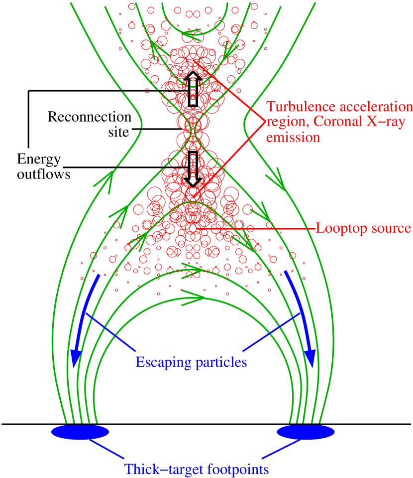
Figure 1.— Sketch of the stochastic acceleration model (Hamilton & Petrosian, 1992; Park & Petrosian, 1995; Petrosian & Liu, 2004) proposed for solar flares. The green curves are magnetic field lines in a possible configuration; the red circles represent turbulence or plasma waves that are generated during magnetic reconnection.

It is well established that many flares have SXR and HXR emission arising both from the source near the top of the loop (loop-top source, e.g., Masuda, 1994; Petrosian et al., 2002; Liu et al., 2004; Jiang et al., 2006; Liu, 2006; Battaglia & Benz, 2006) and from a pair of footpoint sources (e.g., Hoyng et al., 1981; Sakao, 1994; Sui et al., 2002; Saint-Hilaire et al., 2007). The loop-top source is believed to be near the reconnection site and produced by freshly accelerated particles and/or heated plasma. Observations of the expected two distinct X-ray sources above and below the reconnection region have been rarely reported. This may be due to limited sensitivity, dynamic range, and/or spatial resolution of the instruments, because one source may be much dimmer than the other, the two sources may be too close together to be resolved, or both may be much weaker than the footpoints.

Sui & Holman (2003) and Sui et al. (2004) reported a second coronal source that appeared above a stronger loop-top source in the 2002 April 15 flare and in another two homologous flares. They suggested that there was a current sheet existing between the two sources. Recently, in one of the events reported by Sui et al. (2004), Wang et al. (2007) discovered high speed outflows revealed by Doppler shifts measured by the Solar Ultraviolet Measurements of Emitted Radiation (SUMER) instrument on board the Solar and Heliospheric Observatory (SOHO). This provides more evidence of magnetic reconnection. Veronig et al. (2006) also found a second coronal source appearing briefly in the 2003 November 03 X3.9 flare (Liu et al., 2004; Dauphin et al., 2006). Li & Gan (2007) reported another RHESSI flare, occurring on 2002 November 02, that shows a similar double coronal source morphology. They interpreted the two sources as thermal emission because no HXR emission was detected above 25 keV and the footpoints were occulted. In their event, however, the two sources have somewhat different temporal evolution with the flux of the upper source peaking about 18 minutes later than that of the lower source. In radio wavelengths, Pick et al. (2005) reported a double-source structure observed in the 2002 June 02 flare with the multi-frequency Nançay Radio-heliograph (432–150 MHz). Due to its low brightness and/or technical difficulties, X-ray imaging spectroscopy of the weaker coronal source was not available or has not been studied for the above RHESSI events (Sui & Holman, 2003; Sui et al., 2004; Veronig et al., 2006; Li & Gan, 2007).

We report here another flare with two distinct coronal X-ray sources that occurred on April 30, 2002. The brightness of the upper source relative to the lower source is larger and the upper source stays longer ($\sim$12 minutes) than those (3–5 minutes) of Sui et al. (2004). In addition, the footpoints are occulted by the solar limb, and thus the spectra of the coronal sources are not contaminated by the footpoints at high energies. This makes a stronger case for the double coronal source phenomenon and allows for more detailed analysis, including X-ray imaging spectroscopy and temporal evolution of the individual sources. Analysis of the decay phase of this flare was originally reported by Jiang et al. (2006) as an example of suppression of thermal conduction and/or continuous heating attributed to the presence of plasma turbulence. Here we extend the analysis throughout the whole course of the flare.

Early in the flare, the two coronal sources are close together and the source morphology exhibits a double-cusp or “X” shape, possibly indicating where magnetic reconnection takes place. As the flare evolves, the two sources gradually separate from each other. Both sources exhibit energy dependent structure similar to that found for the flares reported by Sui et al. (2004) and Liu et al. (2004). In general, for the lower source, higher-energy emission comes from higher altitudes, while the opposite is true for the upper source. Imaging spectroscopy shows that the two sources have very similar nonthermal components and light curves. These observations suggest that the two HXR/SXR coronal sources are produced by intimately related populations of accelerated/heated electrons resulting from energy release in the same reconnection region, which most likely lies between the two sources. These are consistent with the general picture outlined above. We also find that the two sources have different thermal components, with a lower temperature and larger emission measure for the lower source. Different magnetic topologies and plasma densities of the two sources can be the causes of such differences.

We present the observations and data analysis in §2 and our physical interpretation in §3. We conclude this paper with a brief summary and discussion in §4. Details of specific RHESSI spectral analysis techniques are provided in Appendix A.

2. Observations and Data Analysis

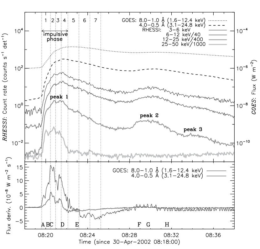
Figure 2.— Top: RHESSI and GOES-10 light curves of the 2002 April 30 M1.4 flare. The RHESSI count rates (left scale) are averaged over every 4 seconds, with scaling factors of 1, 1/40, 1/400, and 1/1000 for the energy bands 3–6, 6–12, 12–25, and 25–50 keV, respectively. The GOES fluxes (right scale) in the bandpass of 8–1 Å (1.6–12.4 keV) and 4.0–0.5 Å (3.1–24.8 keV) are in a cadence of 3 seconds. The vertical dotted lines mark the seven time intervals used for imaging spectroscopy (see Figures 7 and 8). Intervals 1–4 correspond to the impulsive phase according to the 25–50 keV light curve. Three peaks on the 12–25 keV curves are also marked. Bottom: Time derivatives of the GOES fluxes, showing the Neupert-type behavior. The capital letters (A–H) at the bottom mark the central times of the intervals of the images shown in Figure 5. Note that the energy release episode of peak 2 may actually start at $\sim$08:25 UT when the exponential decay rate of the RHESSI light curves (3–25 keV) decreases and the GOES time derivative (8–1 Å) starts to increase.

The event under study, classified as a Geostationary Operational Environment Satellite (GOES) M1.4 flare, started at 08:19 UT on April 30, 2002. Figure 2 (top panel) shows the RHESSI light curves in four energy bands between 3 and 50 keV together with the fluxes of the two GOES channels (1–8 and 0.5–4.0 Å). During the full course of the flare, RHESSI is in the A1 attenuator state, i.e. with the thin shutters in. According to the 12–25 keV light curve, there are three peaks that are progressively weaker and softer. Above 25 keV there is no detectable count rate increase beyond the first peak that we refer to as the impulsive phase.

The temporal trend of the time derivatives (Figure 2, bottom panel) of the GOES fluxes mimics that of the RHESSI 25–50 keV count rate. This type of correlation is known as the Neupert effect (Neupert, 1968) and has been observed in many (but not all) flares (Dennis & Zarro, 1993; Veronig et al., 2005; Liu et al., 2006b). Such flares are usually observed on the solar disk where HXRs are seen from the footpoints, indicating prompt energy release and impulsive heating of the chromosphere by the nonthermal electrons. The hot and dense plasma resulting from the subsequent chromospheric evaporation (Neupert, 1968) then fills the loop and gives rise to the gradual SXR increase (Liu, 2006, Chapter 8). In this flare, however, the footpoints are occulted by the limb (as we show below). Thus, the presence of the Neupert effect here implies that the coronal impulsive HXRs are produced by the same nonthermal electrons that further propagate down to the footpoints and drive chromospheric evaporation there.

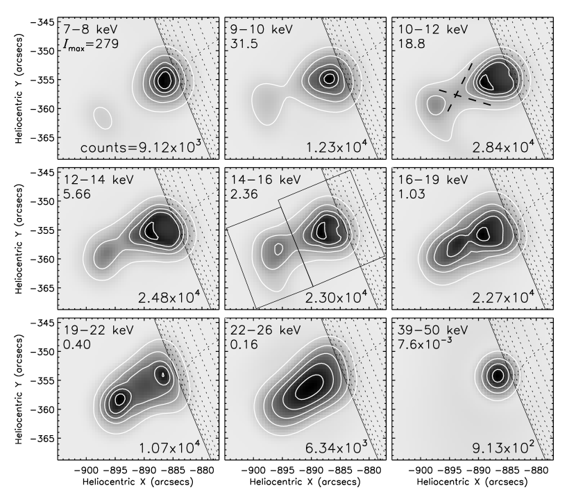
Figure 3.— RHESSI PIXON images in different energy bands at 08:20:27–08:20:56 UT (interval 2 in Figure 2), around the maximum of the main (first) HXR peak. We used the PIXON background model and detectors 3–6 and 8, which yield a resolution of $\sim 4\farcs 6$ determined from the FWHM of the point spread function obtained by simulation. Note that the PIXON algorithm, under favorable conditions, can achieve a resolution as small as a fraction (see Aschwanden et al., 2004, §A8) of the FWHM resolution of the finest detector used ($6\farcs 8$ for detector 3 in our case). The contour levels are 10%, 30%, 50%, 70%, and 90% of the maximum, $I_{\mathrm{\,max}}$ (shown in the upper left corner of each panel, in units of photons cm${}^{-2}\mathrm{\,s}^{-1}\mathrm{\,arcsec}^{-2}$), of each individual image. The numbers in the lower right corners are the total counts accumulated by the detectors used for image reconstruction. The heliographic grid spacing is 1^∘. The boxes shown in the 14–16 keV panel are used to obtain the fluxes and centroids of the two sources in all the images at this time (see text). The two black dashed lines in the 10–12 keV panel forming an “X” show the possible configuration of the reconnecting magnetic field.

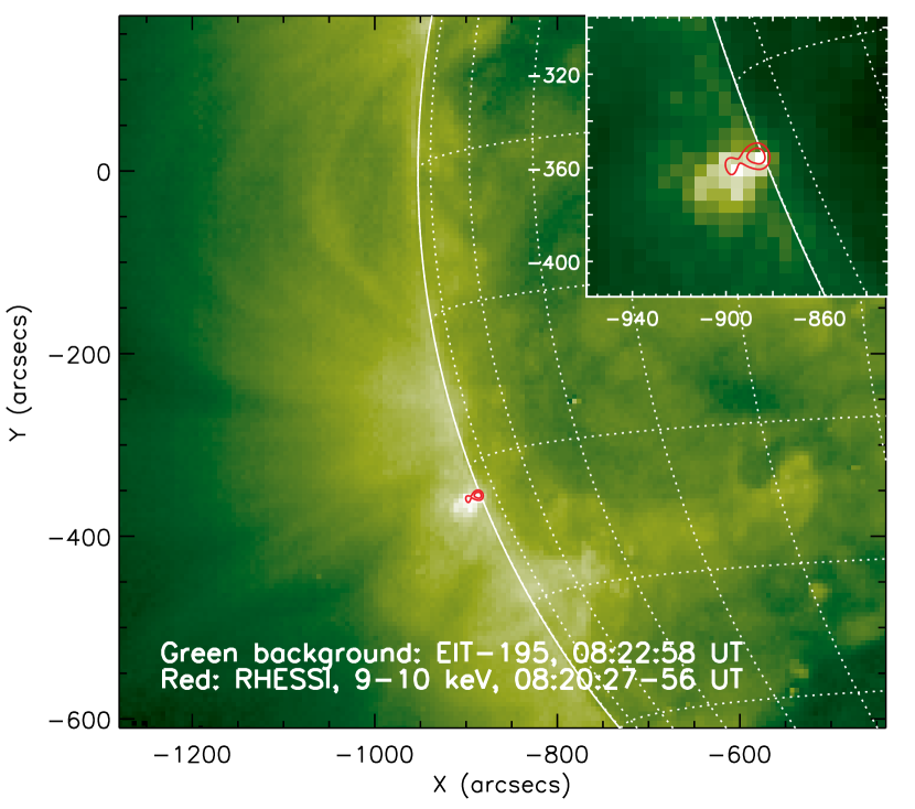
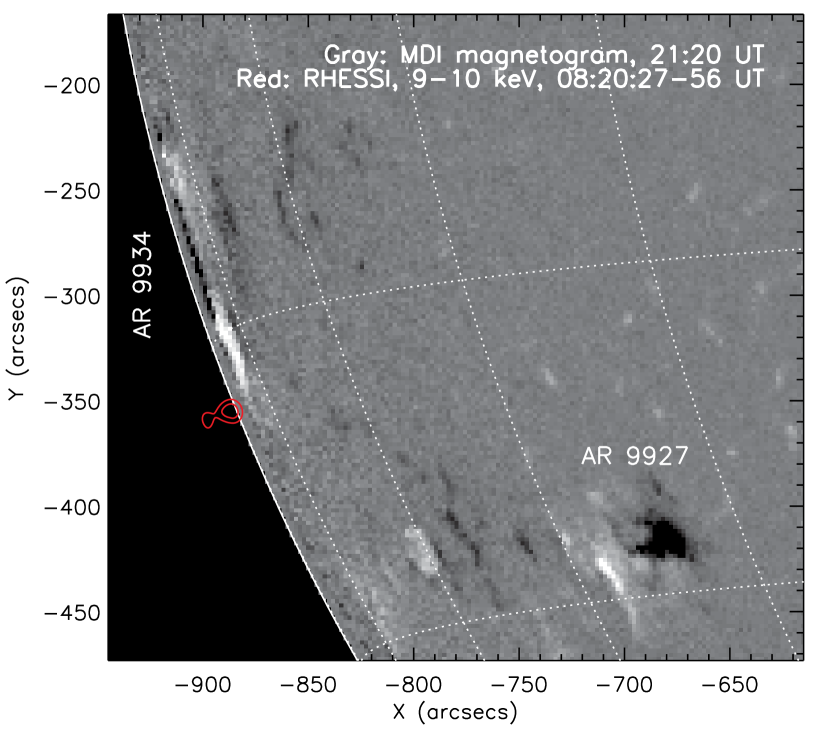
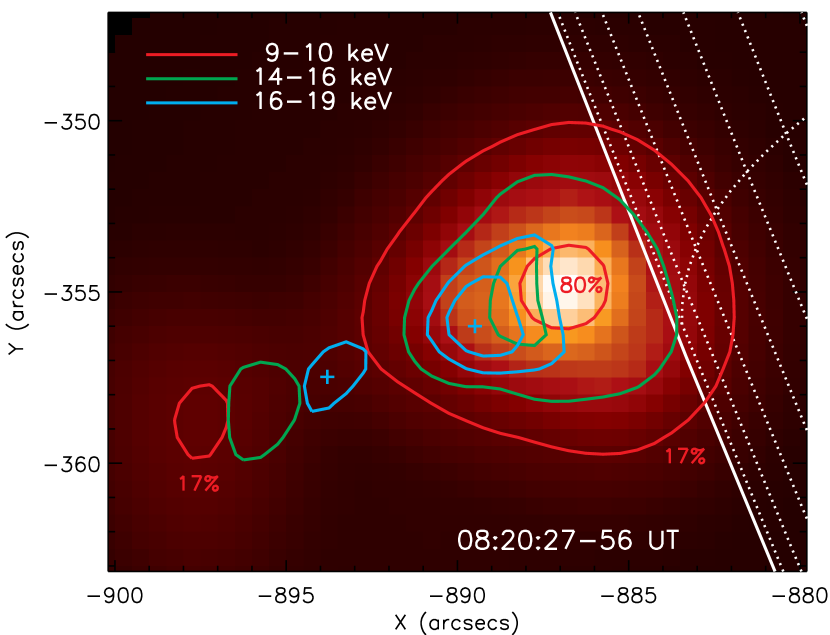
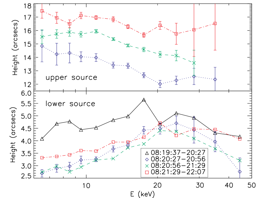
Figure 4.— Upper left: SOHO/EIT 195 Å image at 08:22:58 UT in the background, superimposed with RHESSI contours in red at 9–10 keV and 08:20:27–08:20:56 UT. The insert shows the zoomed view of the RHESSI source and co-spatial EIT emission (with a different color scale for better contrast). Upper right: SOHO/MDI magnetogram taken at 21:20 UT (some 13 hours after the flare), overplotted with the same RHESSI 9–10 keV contours in red. The NOAA active regions (ARs) are labeled. The heliographic grid spacing is 10^∘ in the two upper panels. Lower left: Overlay of images, same as those shown in Figure 3, in three energy bands as indicated in the legend. The contour levels are at 17% & 80% (9–10 keV), 47% & 90% (14–16 keV), and 80% & 90% (16–19 keV) of the maximum brightness of individual images. In each image, two contours appear in the lower coronal source, while only the lower-level contour is present in the upper source because of its faintness. The two plus signs mark the centroids (separated by $4\farcs 6\pm 0\farcs 3$) of the lower and upper 16–19 keV sources inside the 90% and 80% contours, respectively. The heliographic grid spacing is 1^∘. Lower right: Height above the limb of the centroids for the upper and lower coronal sources plotted as a function of energy for time intervals 1–4 marked in Figure 2. Note that during the first interval, only one source is detected and is shown as the lower source. For clarity, uncertainties are shown for only one time interval for the lower source and they are similar at other times.

The spatial morphology of the flare is shown in Figure 3 in X-rays and in Figure 4 in EUV. Figure 3 shows PIXON (Metcalf et al., 1996; Hurford et al., 2002) images at different energies integrated over the interval of 08:20:27–08:20:56 UT (marked #2 in Figure 2) during the first HXR peak. As can be seen, this flare occurred on the east limb, and the X-ray emission at all energies (even as high as 39–50 keV) appeared above the limb, suggesting that the footpoints were occulted. This conclusion is supported by SOHO observations shown in Figure 4. The top left panel shows an EUV Imaging Telescope (EIT) 195 Å image taken at 08:22:58 UT (just two minutes after the RHESSI images in Figure 4). The red contours are for the RHESSI image at 9–10 keV shown in Figure 3. The RHESSI source is co-spatial with the brightening in the EIT image, which is clearly above the limb. The flare occurred near the region where large-scale trans-equatorial loops are rooted, presumably behind the limb. There was no brightening on the disk detected by EIT, nor was an active region seen in the SOHO Michelson Doppler Imager (MDI) magnetograms in the vicinity of this flare. EIT and MDI have spatial resolutions of $2\farcs 6$ and $4\arcsec$, respectively, both better than the $6\farcs 8$ resolution of the finest RHESSI detector (#3) used here. The top right panel of Figure 4 shows the MDI magnetogram at 21:20 UT, about 13 hours after the flare. At this time, NOAA AR 9934 had just appeared on the disk next to the RHESSI source due to the solar rotation. This suggests that the flare took place in this active region when it was still behind the limb. Because of the large size of the active region, it is difficult to determine the possible locations of the footpoints of the flare and to estimate the approximate altitudes of the coronal sources.

2.1. Source Structure: Energy Dependence

Let us now return to Figure 3 and examine in detail the energy-dependent morphology of the flare. At the lowest energy shown (7–8 keV), there are two distinct sources, which we call the lower and upper coronal sources. The centroids of both sources are above the solar limb, and the upper source is dimmer. At a slightly higher energy, 9–10 keV, the sources appear closer together and a cusp shape develops between them. This trend is more pronounced at higher energies (10–19 keV) and the two sources (particularly the lower one) seem to have a feature convex toward each other, mimicking the “X” shape of the magnetic field lines in the standard reconnection model. Meanwhile, the relative brightness of the upper source increases with energy.

The change in source altitude with energy is shown more clearly in the lower left panel of Figure 4. The upper coronal source shifts toward lower altitudes with increasing energy while the lower coronal source behaves oppositely. At 16–19 keV, the two sources, while being spatially resolved, are closest together with their centroids separated by $4\farcs 6\pm 0\farcs 3$ (see Figure 4, lower left).

We can appreciate this more quantitatively by looking at the heights (above the limb) of the centroids of the upper and lower coronal sources as a function of energy. This is shown in the lower right panel of Figure 4. The boxes depicted in the middle panel of Figure 3 were used to obtain the centroid positions. The error bars were obtained from the centroid position uncertainties in the same images reconstructed with the visibility-based forward-fitting algorithm currently available in the RHESSI software. The energy-dependent pattern is clearly present; that is, the centroid of the upper (lower) source shifts to lower (higher) altitudes with increasing energy. We note that, at very high energies ($\gtrsim 20$ keV), this pattern becomes obscure (see Figures 3 and 4), but the uncertainties in the source locations become large due to low count rates.

Three other time intervals during the first HXR peak were also analyzed and the results are plotted in Figure 4, exhibiting similar patterns. At the very beginning of the flare (08:19:37–08:20:27 UT), only one source is visible and we assign its centroid (black triangles) to the lower source since it is the main source. As mentioned earlier, the second and third HXR peaks are weaker and softer, which does not allow for this kind of detailed analysis with narrow energy bins. We defer our physical interpretation of these observations to §3.1.

2.2. Source Structure: Temporal Evolution

We now change our perspective, using relatively wider energy bins as a trade-off for finer time resolution (compared with the above analysis), and examine the temporal evolution of the source structure throughout the full course of the flare.

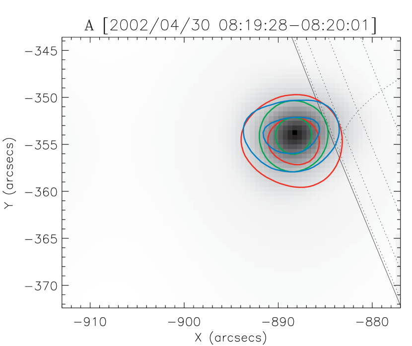
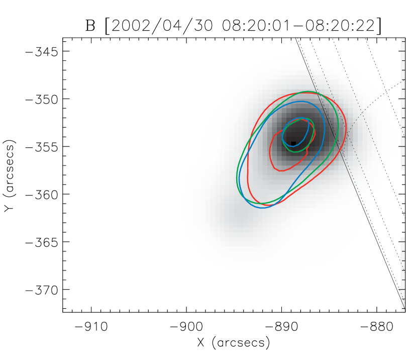
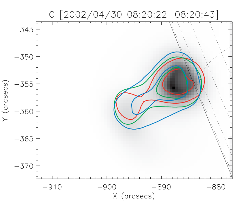
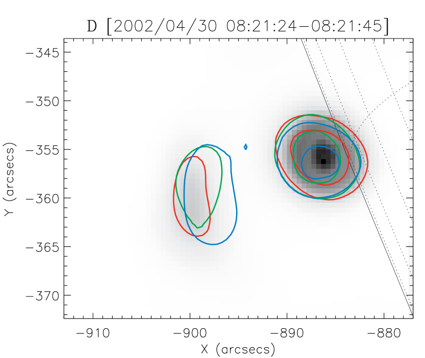
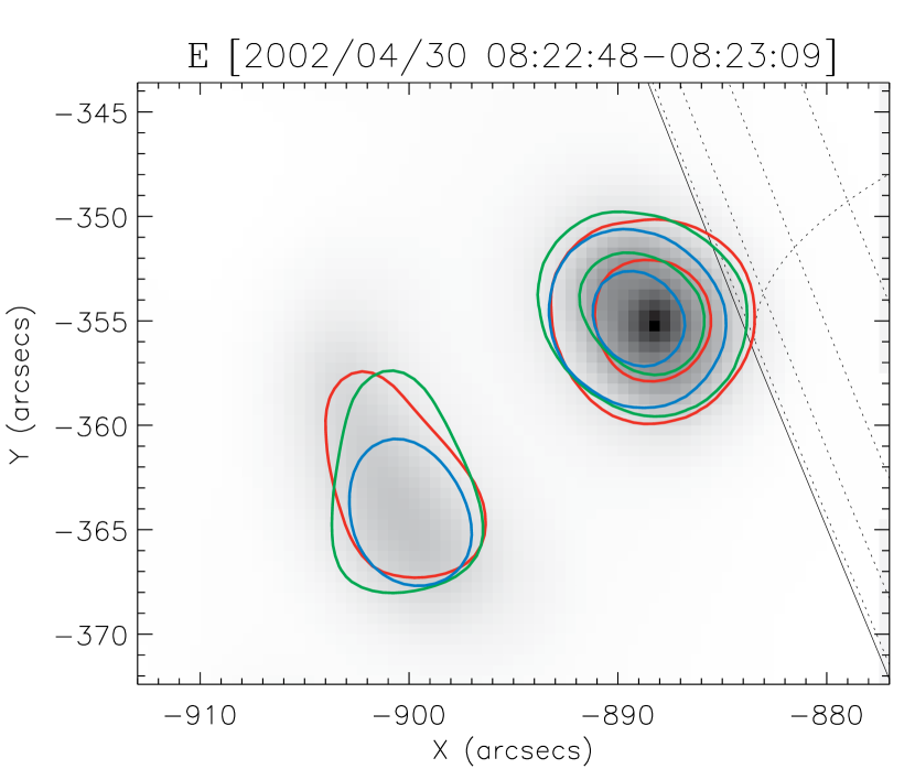
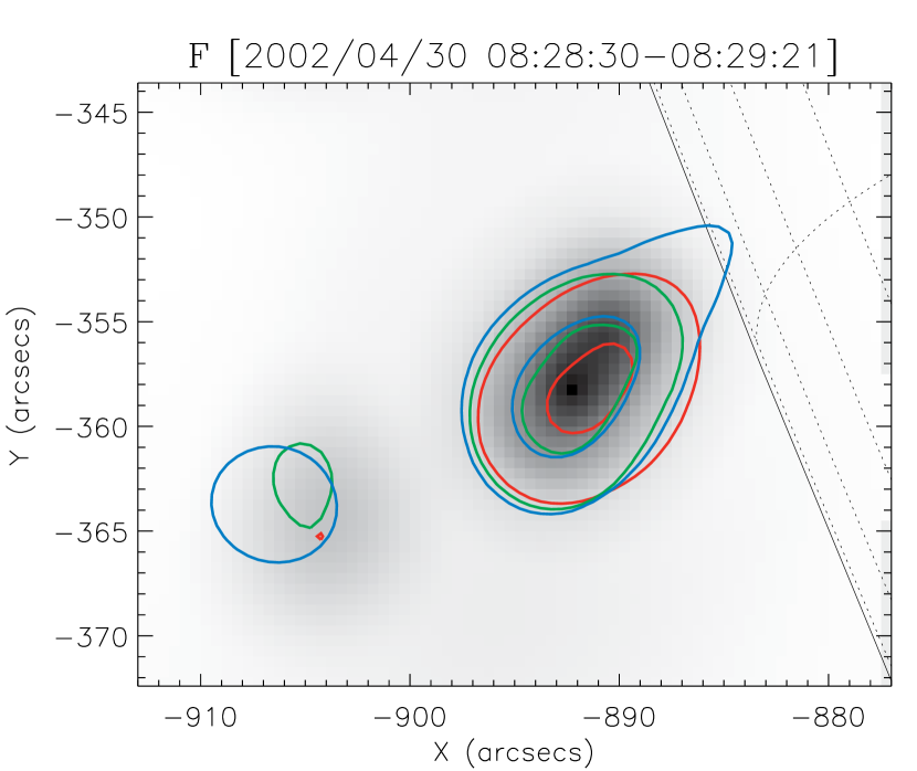
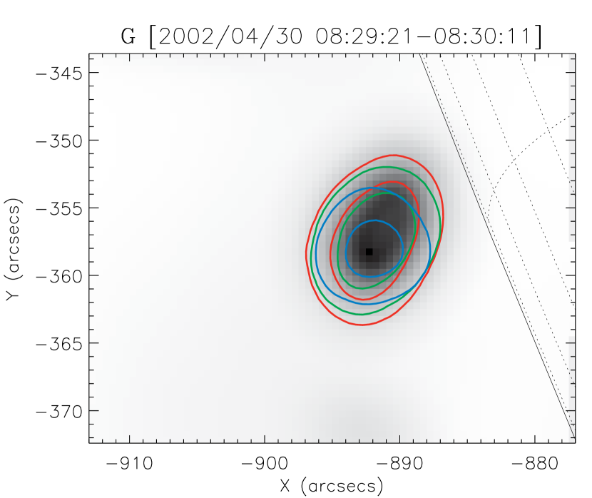
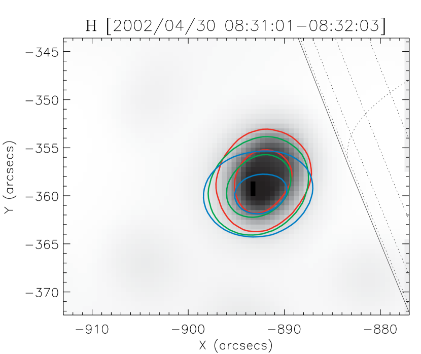
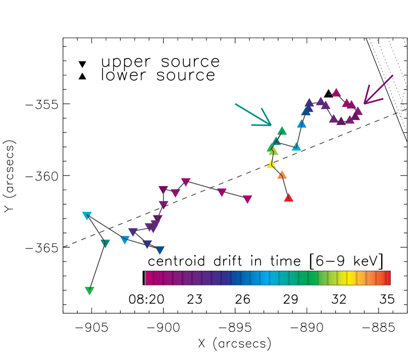
Figure 5.— PIXON images of different energies made with detectors 3–6 and 8 at selected times (i.e., intervals A–H as marked in Figure 2). In each panel, the gray-scale background is at 6–9 keV, while the red, green and blue contours (20% and 70% of the peak flux of each image) are at 9–12, 12–16 and 16–25 keV, respectively. The heliographic grid spacing is 2^∘. The last panel shows the locations of the centroids of the lower and upper 6–9 keV sources at different times indicated by the color bar. The dashed line indicates the radial direction (perpendicular to the limb). The magenta and green arrows point to the centroid locations at the times of the first and second HXR peaks, respectively.

Figure 5 shows the PIXON images taken at 6–9, 9–12, 12–16 and 16–25 keV at eight separate times (labeled A–H in Figure 2). The morphology evolves following the general trend mentioned above. Early (08:19:28-08:20:01 UT, interval A) in the flare, only a single source is visible. During the next time interval (B), the upper coronal source appears at 6–9 keV, but only a single source is evident at higher energies albeit with elongated shapes. In interval C, two distinct coronal sources appear in a dumb-bell shape at all the energies. As time proceeds, both sources move to higher altitudes. This morphology is present for about 12 minutes (from 08:20 to 08:32 UT) until the declining phase of the second peak when only one source is detected, possibly because of the faintness of the upper source and the low count rate. Note that after 08:29 UT the upper source is dimmer than 20% of the maximum of the image and thus does not appear in panels G and H.

The motions of the sources can be seen more clearly from the migration of the centroids. To obtain the centroids and fluxes of the sources, we use contours whose levels are equal to within 5% of the minimum between the two sources so that the contours of the two sources are independent. The last panel in Figure 5 shows the evolution of the centroid positions of the two sources at 6–9 keV. During the first HXR peak (indicated by the magenta arrow), the lower coronal source first shifts to lower altitudes and then ascends. This is consistent with the decrease of the loop-top height early during the flare observed in several other events (Sui & Holman, 2003; Liu et al., 2004; Sui et al., 2004). Meanwhile, the upper source generally moves upwards. Such centroid motions are also present at other energies as shown in the lower right panel of Figure 4. The reversal of the lower source altitude seems to happen again, but less obvious, during the second peak (marked by the green arrow).

We can examine the same phenomenon more quantitatively by checking the height of the source centroid as a function of time at different energies. This is shown in Figure 6a for the upper (left scale) and lower (right scale) coronal sources. We find that, again, the higher-energy emission comes from lower altitudes for the upper source and the lower source shows the opposite trend. The only exception (indicated by the dashed box) to this general behavior occurs for the upper source during the late declining phase of first HXR peak and during the second and third peaks when there are large uncertainties because of low count rates.

At 6–9 keV (red symbols), the altitude of the lower source first decreases at a velocity of $10\pm 2\mathrm{\,km}\mathrm{\,s}^{-1}$, while the altitude of the upper source increases at a velocity of $52\pm 18\mathrm{\,km}\mathrm{\,s}^{-1}$. These are indicated by linear fits (red solid line) during the high flux period. This happens during the rising phase (up to 08:21:14 UT) of the first HXR peak and is followed by an increase of the altitudes of the two sources with comparable velocities ($15\pm 1\mathrm{\,km}\mathrm{\,s}^{-1}$ and $17\pm 4\mathrm{\,km}\mathrm{\,s}^{-1}$ for the lower and upper sources, respectively) during the early declining phase (up to 08:22:59 UT). As time proceeds, the two sources generally continue to move to higher altitudes. The velocity of the lower source drops to $7.6\pm 0.5\mathrm{\,km}\mathrm{\,s}^{-1}$ until 08:28:56 UT, around the maximum of the second HXR peak, and then to $2.3\pm 0.6\mathrm{\,km}\mathrm{\,s}^{-1}$ afterwards. The velocity of the upper source also decreases in general, with some fluctuations most likely due to the large uncertainties mentioned above. The relative motion of the two sources can be seen from the temporal variation of the distance between their centroids as shown in Figure 6b (red asterisks), which undergoes a fast initial increase and then stays roughly constant at $15\arcsec\pm 1\arcsec$ within the uncertainties.

At 12–16 (green) and 16–25 keV (blue), the centroids have a trend similar to those at 6–9 keV, except for the lower coronal source during the early rising phase of the first HXR peak. The initial increase of the height of the “lower” source at about 08:20 UT results from the elongation (see the second panel in Figure 5) of the single source, which could be a combination of the lower and upper sources that are not resolved. The following rapid decrease in height in the next time interval is a consequence of the transition from a single-source to a double-source structure as mentioned earlier. The upper source, on the other hand, rises more rapidly than at 6–9 keV during the HXR rising and early declining phases. Its velocity at 16–25 keV, for example, is $32\pm 3\mathrm{\,km}\mathrm{\,s}^{-1}$ during the interval of 08:21:14–08:22:59 UT. This energy dependence of the rate of rise is consistent with the general trend of the loop-top source observed in several other flares (Liu et al., 2004; Sui et al., 2004). We note in passing that, in addition to the first HXR peak (marked with D₁ in Figure 6), the altitudes of the lower source centroids also appear to first decrease and then increase during two other time periods (D₂ and D₃). This effect is most pronounced at 12–16 and 16–25 keV.

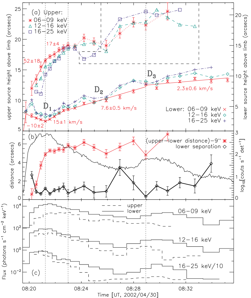
Figure 6.— (a) Height (above the limb) of the centroids at different energies for the upper (left scale) and lower (right scale) coronal sources. The dotted vertical lines separate the different phases according to the motion of the lower source centroid (see text). The red solid lines are linear fits to the data during the corresponding time intervals, with the adjacent red numbers indicating the velocities of the altitude gain in units of $\mathrm{\,km}\mathrm{\,s}^{-1}$. The centroid position of the upper source has large fluctuations and uncertainties during the interval marked by the dashed box. The letters D₁, D₂, and D₃ mark the times when the altitude of the lower source decreases. (b) Left scale: Distance (red asterisks) between the centroids of the two coronal sources at 6–9 keV and separation (diamonds) between the centroids of the lower source at 6–9 and 16-25 keV. The former is shifted downwards by $9\arcsec$. Right scale: Base-10 logarithm of the spatially integrated light curve (counts $\mathrm{\,s}^{-1}$ detector^-1, thin line) at 12–25 keV. (c) Light curves of the upper (dashed) and lower (solid) coronal sources in the energy bands of 6–9, 12–16, and 16–25 keV (divided by 10). The same contours (see text) were used to obtain these light curves and the centroid positions in panel a.

2.3. Spectral Evolution

In this section, we examine the relationship between the fluxes and spectra of the two coronal sources. Figure 6c shows the photon flux evolution at 6–9, 12–16, and 16–25 keV. As evident, the fluxes of the two sources basically follow the same time variation in all three energy bands. The upper coronal source, however, appears later and disappears earlier, presumably due to its faintness and the limited RHESSI dynamic range ($\sim$10:1). It also peaks later at 6–9 keV.

We also conducted imaging spectroscopic analysis for each of the seven time intervals defined in Figure 2. The spectra of the two sources separately and the spatially integrated spectra were fitted with a single-temperature thermal spectrum plus a power-law function. One important step was to fit the spatially integrated spectra of individual detectors separately and then average the results in order to obtain the best-fit parameters and their uncertainties. Interested readers are referred to Appendix A for the technical details of the spectrum fitting procedures used to obtain the results reported here.

Figure 7.— Spectra of the lower and upper coronal sources and the spatially integrated spectra (labeled as “total”) at four times during the major flare peak. The numbers (2, 3, 4, and 5) in the upper-right corners correspond to the numbered time intervals shown in Figure 2. The upper source’s spectra and the total spectra have been shifted downwards by one and three decades, respectively. The horizontal error bars represent the energy bin widths and the vertical error bars are the statistical uncertainties of the spectra. The best fit to the data with a thermal plus power-law model is shown as the dotted (dashed) line for the lower (upper) source. The thermal (dotted) and power-law (dashed) components of the best fit to the total spectra are also shown. The legend indicates the corresponding power-law indexes ($\gamma$) for each spectrum ($\gamma=2$ below the low cutoff energy). The lower portion of each panel shows the ratio of the upper to lower fluxes (asterisk symbols, left scale), and the residuals (solid lines, right scale) of the fit to the spatially integrated spectra, normalized to the $1\sigma$ uncertainty of the measured flux at each energy.

A sample of the resulting spectra of four intervals is shown in Figure 7. Fits to the spatially integrated spectra indicate that the low-energy emission is dominated by the thermal components, while the nonthermal power-law components dominate at high energies. The two components cross each other at an energy that we call $E_{\mathrm{\,cross}}$. The spectra of the two coronal sources measured separately have similar slopes. In general, the ratio of the two spectra (upper source/lower source) is smaller than unity and gradually increases with energy below around $E_{\mathrm{\,cross}}$. This trend can also be appreciated by noting the increasing relative brightness of the upper source when energy increases as shown in Figure 3. This energy-dependent variation of the flux ratio means that the thermal emissions of the two sources are somewhat different not only in emission measure (EM) but also in temperature, because different EMs alone would only affect the normalizations and produce a flux ratio that is independent of energy. We also note that above $E_{\mathrm{\,cross}}$, the ratio stays constant within the larger uncertainties. This means that the nonthermal spectra of the two sources have similar power-law indexes (see Figure 8a).

The reduced $\chi^{2}$ values of the spatially integrated spectra are somewhat large ($\gtrsim$2) partly because we set the systematic uncertainties to be zero as opposed to the default 2%. Another reason was that we averaged the photon fluxes and best-fit parameters over different detectors that have slightly different characteristics. Thus, the averaged model may not necessarily be the best fit to the averaged data (see §A.1, item 9), although the $\chi^{2}$ values of the fits to the individual detectors are usually close to unity. The normalized residuals exhibit some systematic (non-random) variations, as shown in the bottom portion of each panel of Figure 7. This suggests that simple spectrum form adopted here may not represent all the details of the data. However, since we are mainly concerned with the similarities and differences between the spectra of the two coronal sources, such systematic variations would affect both spectra the same way and thus will not alter our major conclusions. More sophisticated techniques, such as the regularization method (Kontar et al., 2004), can be used to obtain better fits to the data, but they are beyond the scope of this paper.

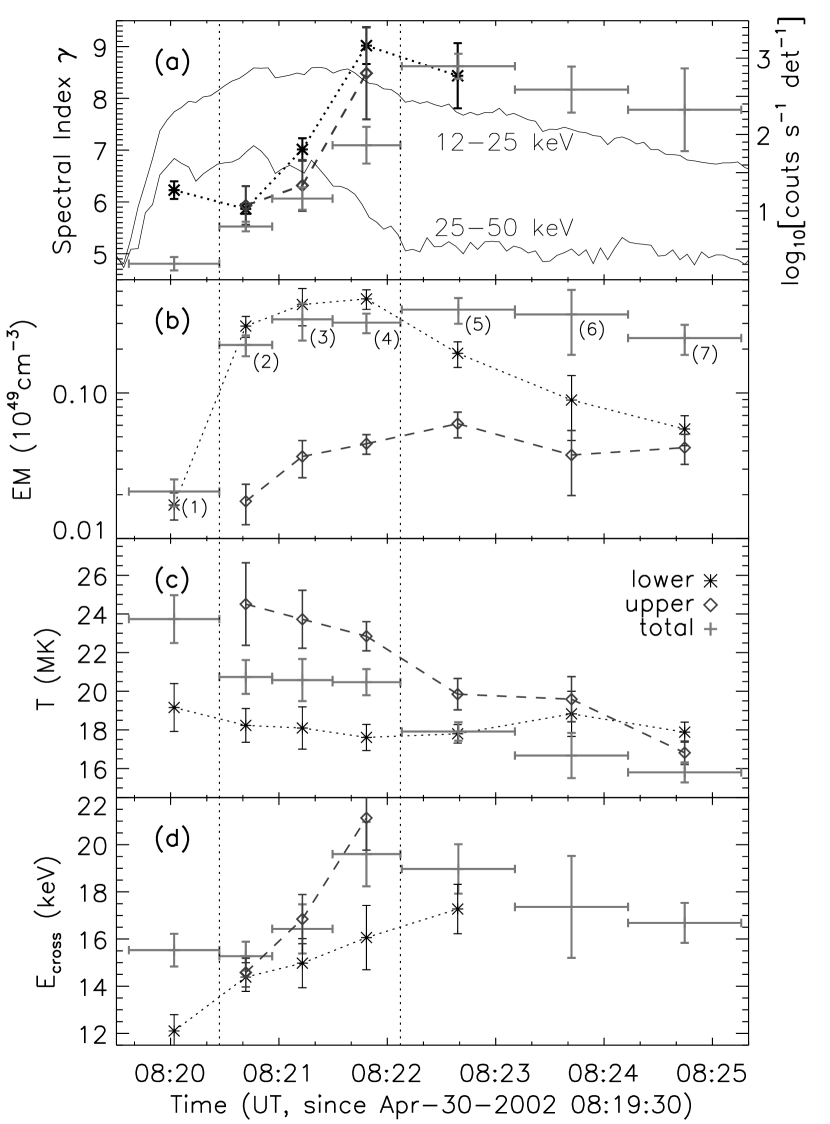
Figure 8.— Evolution of various spectroscopic quantities of the lower (asterisks) and upper (diamonds) coronal sources and the spatially integrated emission (pluses, labeled “total”). The horizontal error bars represent the widths of the time intervals of integration as labeled (1–7) in panel b (also in Figure 2). The two vertical dotted lines mark the boundaries of the time range when both coronal sources are best imaged. This spans the late impulsive phase (see the 25–50 keV light curve). Before and after this time range the imaging spectroscopy has relatively large uncertainties (see text). (a) Spectral indexes (symbols, left scale) of the power-law components of the model fits, together with the 12–25 and 25–50 keV light curves (solid lines, right scale). (b) and (c) Emission measures (in $10^{49}\mathrm{\,cm}^{-3}$) and temperatures (in $10^{6}$ K) of the thermal components of the model fits. (d) The cross-over energy, $E_{\mathrm{\,cross}}$, at which the thermal and power-law components are equal. Note that the values here are the upper limits of $E_{\mathrm{\,cross}}$. This is because we assumed a $\gamma=2$ index for the photon spectrum below the low-energy cutoff, but the power-law component may extend to low energies with a steeper index thus lowering the values of $E_{\mathrm{\,cross}}$.

We now examine the temporal evolution of various spectral characteristics as shown in Figure 8. Let us focus on the late impulsive phase outlined by the two vertical dotted lines. Again, we find that the power-law indexes (Figure 8a) of the two coronal sources are very close, with a difference of $\Delta\gamma\leq 0.7$. The two spectra undergo continuous softening during this stage, and the spatially integrated spectrum follows the same general trend.

Figures 8b and 8c show that the thermal emissions of the two sources are quite different as noted above. The lower coronal source has a larger emission measure but lower temperature than the upper source. As time proceeds, both sources undergo a temperature decrease and emission measure increase. This must be the result of the interplay of continuous heating, cooling by conduction and radiation, and heat exchange between regions of different temperatures within the emission source. Note that the temperature and emission measure of the spatially integrated spectrum, as expected, lie between those of the two sources.

We can further estimate the densities of the two sources using their EMs and approximate volumes. Assuming that the sources are spheres and using the $6\farcs 3$ and $5\farcs 2$ FWHM source sizes obtained from the visibility forward fitting images as the diameters, we obtained the volumes, $V$. We then estimated the lower limits of the densities ($n=\sqrt{\mathrm{\,EM}/[Vf]}$, assuming a filing factor $f$ of unity) of the lower and upper sources at 08:20:27-08:20:56 UT to be $2.4\times 10^{11}$ and $8.0\times 10^{10}\mathrm{\,cm}^{-3}$, respectively.

Figures 8d shows the history of the cross-over energy $E_{\mathrm{\,cross}}$. In general, the lower source has a lower $E_{\mathrm{\,cross}}$ because of its lower temperature. The $E_{\mathrm{\,cross}}$ values of both sources increase with time because the thermal emission becomes increasingly dominant, as seen in many other flares. Physical interpretation of these observations is presented in the next section.

3. Interpretation and Discussion

3.1. Energy Dependence of Source Structure

The energy-dependent source morphology presented in §2.1 (see Figure 4, lower left) is similar to that reported by Sui & Holman (2003) and Sui et al. (2004) and interpreted as magnetic reconnection taking place between the two coronal sources. In their interpretation, plasma with a higher temperature is located closer to the reconnection site than plasma with a lower temperature. This can result in higher-energy emission coming from a region closer to the reconnection site while lower-energy emission comes from a region further away, provided that the emission is solely produced by thermal emission (free-free and free-bound) and the lower-temperature plasma has a higher emission measure.

Our interpretation is somewhat different, particularly for this flare. Regardless of the emission nature (thermal or nonthermal) of the HXRs, the energy-dependent source structure here simply means harder (flatter) photon spectra closer to the reconnection site, which can give rise to a higher weighting there at high energies for the centroid calculations. A larger spatial gradient of the spectral hardness would lead to a larger separation of the emission centroids at two given photon energies, and a zero gradient (uniform spectrum) means no separation. As we have seen in §2.3, both coronal sources have substantial power-law (presumably nonthermal) tails (Figure 7), which makes a purely thermal interpretation improbable. In the framework of the stochastic acceleration model (Hamilton & Petrosian, 1992; Miller et al., 1996), one expects both heating of plasma and acceleration of particles into a nonthermal tail to take place. As shown in Petrosian & Liu (2004), higher levels of turbulence tend to produce harder electron spectra or more acceleration and less heating. One expects a higher turbulence level near the X-point of the reconnection site than further away. Consequently, there will be more acceleration and thus stronger nonthermal emission near the center, but more heating and thus stronger thermal emission further away from the X-point. In other words, the electron spectra and thus the observed photon spectra will be harder closer to the reconnection site. This physical picture is sketched in Figure 9.

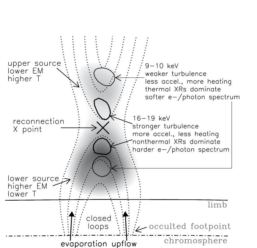
Figure 9.— Schematic of the physical scenario (see text) superimposed on the RHESSI observations, as a manifestation of the stochastic acceleration model illustrated in Figure 1. The 14–16 keV PIXON image at 08:20:27–08:20:56 UT is the gray background, overlaid with the simultaneous 9–10 (thin) and 16–19 keV (thick) contours. These are the same images shown in the lower left panel of Figure 4, with their orientation rotated for demonstration purposes. The hand-drawn dotted curves represent a possible magnetic field configuration.

The observations here support the above scenario. As shown in Figure 7, below the critical energy $E_{\mathrm{\,cross}}$ (say, $\sim$15 keV for 08:20:27–08:20:56 UT), the emission is dominated by the thermal component, and the two sources are further apart at lower energies (see Figure 4, lower panels). This translates to the outer region away from the center of the reconnection site being mainly thermal emission at low energies. Above $E_{\mathrm{\,cross}}$, on the other hand, the power-law component dominates. The two sources being closer together at higher energies thus means that the region near the center is dominated by nonthermal emission (see Figure 9).

We note that the small centroid separation of $4\farcs 6\pm 0\farcs 3$ (Figure 4, lower left) identifies a region within which the center of reconnection activity is located. To our knowledge, this is the smallest ($3.3\pm 0.2$ Mm) feature of the reconnection region yet resolved by X-ray observations on the Sun.

3.2. Temporal Evolution of Source Structure

Figure 6b shows the separation (black diamonds) between the centroids of the lower coronal source at 6–9 and 16–25 keV, together with the 12–25 keV light curve. These two curves seem to be anti-correlated such that this separation becomes smaller when the HXR flux is larger. This is consistent with that reported by Liu et al. (2004, Figure 1) in a much brighter (X3.9) flare where this effect was more pronounced. This trend was also present in two of the three homologous flares reported by Sui et al. (2004).

In our earlier publication (Liu et al., 2004), we suggested that the anti-correlation indicates a smaller (more homogeneous) spatial gradient of turbulence density or particle acceleration rate around the peak of the impulsive phase, owing to the presence of a higher turbulence level. Here, we further note that such a spatial distribution of acceleration rate can result from the interplay of various physical processes (with different spatial distributions and time scales) that contribute to energy release, dissipation, and redistribution. Processes that can carry energy away from the acceleration region include damping of turbulence (waves), escape of accelerated particles, thermal conduction, and radiative loss. Detailed modeling is required to offer a self-contained physical explanation for the observational feature presented here.

3.3. Spectral Characteristics

The temporal correlation of the light curves (Figure 6c) and the similar power-law spectral components (Figures 7 and 8a) of the two coronal sources, when taken together, suggest that these HXR emissions are produced by the nonthermal electrons that are accelerated by the same mechanism (presumably stochastic acceleration by similar turbulence) following the reconnection process. Such a correlation provides more direct evidence and a more complete picture for the interpretation outlined above in §3.1.

As we noted in §2.3, the coronal sources have quite different thermal emissions, with the lower source having a higher EM but lower temperature. There are several possible reasons why this can happen: (1) The lower source resides at a lower altitude where the local density may be slightly higher in the gravitationally stratified atmosphere. The difference between the heights of the two sources is on the order of 10 Mm, which is a fraction of the coronal density scale height ($\gtrsim$60 Mm, the quiet Sun value). Thus, the density difference due to height variation is no more than about 15%. This is not sufficient to account for the large difference in density between the two sources noted earlier. (2) As shown in Figure 9, the two coronal sources lie below and above the X point of the reconnection region. It is most likely that the lower source is located at the top of the flaring loop that is magnetically connected to the chromosphere. This allows the chromosphere to supply dense material to the lower source along the magnetic field lines during chromospheric evaporation. The evaporated plasma, although heated, is still relatively cooler than the hot plasma near the reconnection site in the corona. (3) In addition, thermal conduction and plasma convection can readily carry heat away from the lower source down the magnetic loop to the cool chromosphere. All the three reasons contribute to the higher EM and lower temperature of the lower coronal source. In contrast, the upper source may be magnetically disconnected from or more remotely connected to the solar surface. The lower density material of the upper source can thus be heated to a higher temperature due to the lack of a direct supply of cool material and the reduced thermal conduction to the chromosphere.

We have also noted that the nonthermal components of the two coronal sources have similar spectral indexes, but the upper source is weaker. The spectral indexes could not always be determined for both sources seen in other similar events (Sui & Holman, 2003; Sui et al., 2004; Veronig et al., 2006; Li & Gan, 2007), but the upper source was always the weaker of the two. Here we discuss the possibilities that can lead to the weaker nonthermal radiation of the upper source in particular and its low surface brightness in general. In the framework of the stochastic acceleration model, all the processes involved in producing the observed emission – the rate of generation of turbulence, the spectrum of turbulence, the rate of acceleration and emission – depend on the temperature, density, and the magnetic field strength and geometry. As we mentioned above, the temperature, density, and field geometry of the two coronal sources are different. The magnetic field strength most likely decreases with height. Consequently, we expect different HXR intensities from the two sources. For example, the lower plasma density in the upper source will result in lower surface brightness for both thermal and nonthermal bremsstrahlung emission. Magnetic topology can have similar effects. The electrons responsible for the upper source are likely to be on open field lines or on field lines that connect back to the chromosphere more remotely (e.g., Liu et al., 2006a) and thus produce their X-ray emission in a more spatially diffuse region. In contrast, for the lower source, the electrons are confined in the closed loop. In addition, as noted above, chromospheric evaporation can further increase the density in the loop, enhancing the density effect mentioned here. These factors, again, lead to lower surface brightness for the upper source. Finally, the rate of acceleration or heating depends primarily on the strength of the magnetic field (Petrosian & Liu, 2004), so that the relatively weaker magnetic field of the upper source may result in slower acceleration and thus weaker nonthermal emission. A large sample of this type of flares is required to confirm or reject this explanation.

We should emphasize that since the radiating electrons in both sources are the direct product of the same acceleration mechanism, they share common signatures. This would explain the spectral similarity of the nonthermal emissions of the two coronal sources. The thermal X-ray emitting plasma, however, in addition to direct heating by turbulence, involves many other indirect or secondary processes, such as cooling by thermal conduction and hydrodynamic effects (e.g., evaporation in the closed loop). Therefore, the two thermal sources exhibit relatively large differences in their temperatures and emission measures.

4. Concluding Remarks

We have performed imaging and spectral analysis of the RHESSI observations of the M1.4 flare that occurred on April 30, 2002. Two correlated coronal HXR sources appeared at different altitudes during the impulsive and early decay phases of the flare. The long duration ($\sim$12 minutes) of the sources allows for detailed analysis and the results support that magnetic reconnection and particle acceleration were taking place between the two sources. Our conclusions are as follows.

1. Both coronal sources exhibit energy-dependent morphology. Higher-energy emission comes from higher altitudes for the lower source, while the opposite is true for the upper source (Figures 3 and 4). This suggests that the center of magnetic reconnection is located within the small region between the sources.

2. The energy-dependent source structure (Figure 4), combined with spectrum analysis (Figure 7), implies that the inner region near the reconnection site is energetically dominated by nonthermal emission, while the outer region is dominated by thermal emission. This observation, in the framework of the stochastic acceleration model developed by Hamilton & Petrosian (1992) and Petrosian & Liu (2004), supports the scenario (Figure 9) that a higher turbulence level and thus more acceleration and less heating are located closer to the reconnection site.

3. The light curves (Figure 6c) and the shapes of the nonthermal spectra (Figures 7 and 8a) of the two X-ray sources obtained from imaging spectroscopy are similar. This suggests that intimately related populations of electrons, presumably heated and accelerated by the same mechanism following energy release in the same reconnection region, are responsible for producing both X-ray sources.

4. The thermal emission indicates that the lower coronal source has a larger emission measure but lower temperature than the upper source (Figures 8b and 8c). This is ascribed to the expected different magnetic connectivities of the two sources with the solar surface and the associated different plasma densities.

5. During the rising phase of the main HXR peak, the lower source (at 6–9 keV) moves downwards for nearly two minutes at a velocity of $10\pm 2\mathrm{\,km}\mathrm{\,s}^{-1}$, while the corresponding upper source moves upwards at $52\pm 18\mathrm{\,km}\mathrm{\,s}^{-1}$ (Figure 6a). During the early HXR declining phase, the two sources move upwards at comparable velocities ($15\pm 1\mathrm{\,km}\mathrm{\,s}^{-1}$ vs. $17\pm 4\mathrm{\,km}\mathrm{\,s}^{-1}$) for another two minutes. Afterwards, both sources generally continue to move upwards with gradually decreasing velocities throughout the course of the flare, with some marginally significant fluctuations.

6. For the lower source, the separation between the centroids of the emission at different energies seems to be anti-correlated with the HXR light curve (Figure 6b), which is consistent with our earlier finding (Liu et al., 2004). In the stochastic acceleration model, such a feature suggests that a stronger turbulence level (thus a larger acceleration or heating rate and a higher HXR flux) is associated with a smaller spatial gradient (i.e., more homogeneous) of the turbulence distribution or of the electron spectral hardness.

All the above conclusions fit the picture of magnetic reconnection taking place between the two sources as illustrated in Figure 9. This is another, yet stronger, case of a double-coronal-source morphology observed in X-rays, in addition to the five other events reported by Sui & Holman (2003), Sui et al. (2004), Veronig et al. (2006), and Li & Gan (2007).

The general variation with height of the coronal emission raises some interesting questions and provides clues to the energy release and acceleration processes.

The fact that there are two sources rather than one elongated continuous source suggests that energy release takes place primarily away from the “X” point of magnetic reconnection. This can be explained by the following scenario. One may envision that the reconnection gives rise to an electric field which results in runaway beams of particles. This is an unstable situation and will lead to the generation of plasma waves or turbulence, which can then heat and accelerate particles some distance away from the “X” point.

In addition, the energy-dependent structure of each source (i.e., higher energy emission being closer to the “X” point) that extends over a region of $\lesssim 10\arcsec$ suggests that energy release and some particle acceleration occurs in this region. This also indicates that the turbulence level or acceleration rate decreases with distance from the “X” point, which results in softer electron spectra further away from that point. In other words, this observation suggests that the usually observed loop-top source is part of the acceleration region that resides in the loop and has some spatial extent, which is consistent with the recent study reported by Xu et al. (2008). (In their cases, the second coronal source at even higher altitudes above the reconnection site were not detected presumably because of the low total intensity and/or surface brightness.)

Our conclusions do not support the idea that particles are accelerated outside the HXR source before being injected into the loop. Moreover, the observations here are contrary to the predictions of the collisional thick-target model (e.g., Brown, 1971; Petrosian, 1973), which has been generally accepted for the footpoint emission and was recently invoked by Veronig & Brown (2004) to explain the bulk coronal HXRs in two flares described by Sui et al. (2004). In such a model, one expects higher-energy emission to come from larger distances from the acceleration site (e.g., see Liu et al., 2006b, for HXRs from the legs and footpoints of a flare loop) due to the transport effects mentioned in §3.1. The electron spectrum becomes progressively harder with distance (because low-energy electrons lose energy faster). This disagrees with the observations of the flare presented here and of the two flares reported by Sui et al. (2004).

We note in passing that there is a common belief that the “Masuda” type of “above-the-loop” sources (Masuda et al., 1994) constitutes a special class of HXR emission. We should point out that the “Masuda” source is most likely an extreme case of the lower coronal source observed here and of the commonly observed loop-top sources that exhibit harder spectra higher up in the corona (e.g., Sui & Holman, 2003; Liu et al., 2004; Sui et al., 2004). We also emphasize that some type of trapping is required to confine high-energy electrons in the corona while allowing some electrons to escape to the chromosphere (see Figure 1). Coulomb collision in a high-density corona cannot explain simultaneous high-energy coronal and footpoint emission at energies as high as 33–54 keV in the Masuda case. The stochastic acceleration model, on the other hand, provides the required trapping by turbulence that can scatter particles and accelerate them at the same time (Petrosian & Liu, 2004; Jiang et al., 2006).

Finally, besides the stochastic acceleration model, other commonly cited mechanisms, such as acceleration by shocks (e.g., Tsuneta & Naito, 1998) and/or DC electric fields (e.g., Holman, 1985; Benka & Holman, 1994), may or may not be able to explain the energy-dependent source structure presented here. A rigorous theoretical investigation of these models is required to evaluate their viability.

Appendix A Appendix: RHESSI Spectral Analysis

We document in this section the specific procedures adopted to obtain the spatially integrated spectra throughout the flare and the spatially resolved spectra of the two individual coronal sources during the first HXR peak. These procedures are refinements to the standard RHESSI image reconstruction (Hurford et al., 2002) and spectral fitting (Smith et al., 2002) techniques that are implemented in the Interactive Data Language (IDL) routines available in the SolarSoftWare (SSW, Freeland & Handy, 1998). Specific analysis routines are described by (Schwartz et al., 2002) and in various documents on the RHESSI web site at http://hesperia.gsfc.nasa.gov/rhessidatacenter/. The procedures described here can be readily adopted for general RHESSI spectral analysis tasks.

A.1. Spatially Integrated Spectra

For the spatially integrated spectra, we used the standard forward fitting method implemented in the object-oriented routine called Object Spectral Executive (OSPEX) and described in Brown et al. (2006). OSPEX uses an assumed parametric form of the photon spectrum and finds parameter values that provide the best fit in a $\chi^{2}$ sense to the measured count-rate spectrum in each time interval.

In analyzing the RHESSI spatially integrated count-rate spectra, we took advantage of the fact that RHESSI makes nine statistically independent measurements of the same incident photon spectrum with its nine nominally identical detectors. By analyzing the data from each detector separately, up to nine values can be obtained for each spectral parameter. The scatter of these values about the mean then gives a more realistic measure of the uncertainty than can be obtained from the best fit to the spectrum summed over all detectors. In addition, treating each detector separately allows us to use the 1/3 keV wide “native” energy bins of the on-board pulse-height analyzers for each detector. This avoids the energy smearing inherent in averaging together counts from different detectors that have different energy bin edges and sensitivities. We limited the total number of energy bins by using the 1/3 keV native bins only where they are needed, i.e., between 3 and 15 keV. This provides the best possible energy resolution that is important in measuring the iron and iron-nickel line features at $\sim$6.7 and $\sim$8 keV, respectively (Phillips, 2004), and the instrumental lines at $\sim$8 and $\sim$10 keV. We used 1 keV wide energy bins (three native bins wide) at energies between 15 and 100 keV, where the highest resolution was not needed to determine the parameters of the continuum emission in this range.

We recommend the following sequential steps, which we generally followed, to obtain the “best-fit” values of the spectral parameters and their uncertainties in each time interval throughout the flare.

1. Select a time interval that covers all of the RHESSI observations for the flare of interest. Also include times during the neighboring RHESSI nighttime just before and/or just after the flare for use in determining the nonsolar background spectrum.

2. Accumulate count-rate spectra corrected for live time, decimation, and pulse pile-up (Smith et al., 2002, although it is best to correct pile-up in step 6 below) for each of the nine detectors in 4-s time bins (about one spacecraft spin period) for the full duration selected in step 1 above. A full response matrix, including off-diagonal elements, is generated for each detector to relate the photon flux to the measured count rates in each energy bin.

3. Import the count-rate spectrum and the corresponding response matrix for one of the detectors into the RHESSI spectral analysis routine, OSPEX. We used detector 4 since it has close to the best energy resolution of all the detectors.

4. Select time intervals to be used in estimating the background spectrum and its possible variation during the flare. In general, nighttime data must be used if the attenuator state changes during the flare; otherwise pre- and/or post-flare spectra can be used. Account can be taken of orbital background variations during the flare by using a polynomial fit to the background time history in selectable energy ranges or by using the variations at energies above those influenced by the flare. For this event, since the thin attenuator was in place for the whole duration of the flare a pre-flare interval was used for background estimation.

5. Select multiples of the 4-s time intervals used in step 2 that are long enough to provide sufficient counts and short enough to show the expected variations in the spectra as the flare progresses. Be sure that no time interval includes an attenuator change. For this event, we selected the seven time intervals marked in Figure 2 covering the first HXR peak.

6. Fit the spectrum for the interval near the peak of the event to the desired functional form. Spectra can be fitted to the algebraic sum of a variety of functional forms, ranging from simple isothermal and power-law functions to more sophisticated models, such as various multi-thermal models and thin- and thick-target models with a power-law electron spectrum having sharp low-energy and high-energy cutoffs. In our case, we assumed an isothermal component plus a double power-law to provides acceptable fits to the measured count-rate spectra in most cases. This simple two-component model is sufficient to capture the key physics for this flare, i.e., to estimate the relative contributions of the thermal and nonthermal components of the X-ray emission.

   The isothermal spectrum was based on the predictions using the CHIANTI package (v. 5.2, Dere et al., 1997; Young et al., 2003) in SSW with Mazzotta et al. (1998) ionization balance. The iron and nickel abundances were allowed to vary about their coronal values to give the best fit to the iron features in the spectra.

   For simplicity, we set the power-law index below the variable break energy to be fixed at $\gamma=2$ to approximate a flat (constant) electron flux below a cutoff energy. The value of $\gamma$ above the break energy and the break energy itself were both treated as free parameters in the fitting process.

   We also included several other functions to accommodate various instrumental effects. These included two narrow Gaussians near 8 and 10 keV, respectively, to account for two instrumental features that may be L-shell lines from the tungsten grids. The thin attenuator was in place during the entire course of the flare thus restricting us from fitting the spectra below $\sim$6 keV.

   Another routine available in OSPEX was used to both offset the energy calibration and change the detector resolution to better fit the iron-line feature at $\sim$6.7 keV. This is important at high counting rates when the energy scale can change by up to $\sim$0.3 keV.

   Pulse pile-up can best be corrected for at this stage using a separate routine with count-rate dependent parameters although this is still in the developmental stage and was not used for this paper. However, the average live time (between data gaps) during the impulsive peak (interval 1, 08:20:27–08:20:56 UT) of this M1.4 flare was 93.4%. This is to be compared with the values of 55% and 94% for the 2002 July 23 X4.8 flare and the 2002 February 20 C7.5 flare, respectively. In addition, the estimated ratio of piled-up counts to the total counts is below 10% at all energies, indicating very minor pile-up effects on the spectra of this event. A more detailed account on estimating pile-up severity can be found in Liu et al. (2006b, §2.1) and particularly for imaging spectroscopy in Liu et al. (2007).

   It is important to use good starting values of the parameters to ensure that the minimization routine converges on the best-fit values. These were obtained for detector 4 in the interval at the peak of the flare by experienced trial and error.

7. Once an acceptable fit (reduced $\chi^{2}\lesssim{2}$, with the systematic uncertainties set to zero) is obtained to the spectrum for the peak interval, OSPEX has the capability to proceed either forwards or backwards in time to fit the count-rate spectra in other intervals using the best-fit parameters obtained for one interval as the starting parameters to fit the spectrum in the next interval. This reduces the time taken to fit each time interval but various manual adjustments are usually required to the fitted energy range, the required functions, etc., in specific intervals to ensure adequate fits in each case with acceptable values of $\chi^{2}$.

8. The best-fit parameters found for each time interval for the one detector chosen in step 3 are now used as the starting parameters in OSPEX for the other detectors. In this way, acceptable fits can be obtained in each time interval for all nine detectors. In practice, it is usually not possible to include detectors 2, 5, or 7 in this automatic procedure since they have higher energy thresholds and/or poorer resolution compared to the other detectors.

9. The different best-fit values (in practice, only six were obtained) of each spectral parameter can now be combined to give a mean and standard deviation. These values then constitute the results of this spectral analysis and can be used for further interpretation as indicated in the body of the paper. For display purposes, it is important to show the best-fit photon spectrum computed using these mean parameters with some indication of the photon fluxes determined in each energy bin from the measured count rates. For this purpose, we have chosen to display the photon fluxes averaged over over all detectors used in the analysis (all but detectors 2, 5, and 7). The photon flux of each detector was determined by taking the count rate and folding it through the corresponding response matrix with the assumed photon spectrum having the best-fit parameters. This gives a reasonable representation but it is well known that data points determined in this way are “obliging” and follow the assumed spectrum (Fenimore et al., 1983, 1988). Hence, such plots (Figure 7) should be viewed with caution. Also note that the $\chi^{2}$ values of the averaged photon fluxes are not necessarily representative of the independent fits to the data of individual detectors.

A.2. Spatially Resolved Spectra

In order to determine the photon spectra of the two distinct sources seen in the X-ray images, we used RHESSI ’s imaging spectroscopy capability and carried out the following steps.

1. We select the same seven intervals (marked in Figure 2) as those used for the spatially integrated spectra.

2. For each selected time interval, images in narrow energy bins ranging from 1 keV wide at 6 keV to 11 keV wide at 50 keV were constructed using the computationally expensive PIXON algorithm (Metcalf et al., 1996), which gives the best photometry and spatial resolution (Aschwanden et al., 2004) among the currently available imaging algorithms. Detectors 3, 4, 5, 6, and 8 covering angular scales between $6\farcs 8$ and $106\arcsec$ were used to allow the two sources to be clearly resolved. No modulation was evident in the detector 1 and 2 count rates, showing that the sources had no structure finer than the $3\farcs 9$ FWHM resolution of detector 2.

3. The PIXON images were imported into OSPEX for extracting fluxes of individual sources. Note that the images are provided in units of [photons $\mathrm{\,cm}^{-2}\mathrm{\,s}^{-1}\mathrm{\,keV}^{-1}\mathrm{\,arcsec}^{-2}$] using only the diagonal elements of the detector response matrix to convert from the measured count rates to photon fluxes. OSPEX converts the images back to units of [counts $\mathrm{\,cm}^{-2}\mathrm{\,s}^{-1}\mathrm{\,keV}^{-1}\mathrm{\,arcsec}^{-2}$] using the same diagonal elements and then uses the full detector response matrix, including all off-diagonal elements, to compute the best-fit photon spectrum (photons $\mathrm{\,cm}^{-2}\mathrm{\,s}^{-1}\mathrm{\,keV}^{-1}$) for each source separately. The summed count rates in the two boxes shown in the middle panel of Figure 3 around the average positions of the two sources were accumulated separately for each image in each energy bin. The boxes were adjusted accordingly for each time interval if the sources moved. (Note that only a single box was used for Interval 1 when only the lower source was detected.)

4. The uncertainties in the count rates were calculated from the PIXON error map based on $\chi^{2}$ variations of the reconstructed image (see Liu, 2006, §A.2). The errors were originally obtained in photon space and then converted in the same way described above to count space where the actual fitting was performed.

5. The two independent count-rate spectra, one for each source, were then fitted independently to the same functions used for the spatially integrated spectra as described earlier. We further demand that the iron abundance of the thermal component and the break energy of the double power-law are fixed at the values given by the fit to the corresponding spatially integrated spectrum in the same time interval. This makes the spectra directly comparable for our purposes. Note that the error bars of the imaging spectral parameters are obtained from the $\chi^{2}$ variation during the fitting procedure. At times when such an error is smaller than that of the corresponding spatially integrated spectrum, the latter value is used instead.

Finally, for a self-consistency check, we have compared the sum of the imaging spectra of the two sources with the spatially integrated spectrum and found they are consistent. The only exception is at the low energies ($\lesssim$10 keV) where the imaging spectra do not have enough resolution to see the iron-line feature.

References

- Aschwanden et al. (2004) Aschwanden, M. J., Metcalf, T. R., Krucker, S., Sato, J., Conway, A. J., Hurford, G. J., & Schmahl, E. J. 2004, Sol. Phys., 219, 149
- Battaglia & Benz (2006) Battaglia, M. & Benz, A. O. 2006, A&A, 456, 751
- Benka & Holman (1994) Benka, S. G. & Holman, G. D. 1994, ApJ, 435, 469
- Brown (1971) Brown, J. C. 1971, Sol. Phys., 18, 489
- Brown et al. (2006) Brown, J. C., Emslie, A. G., Holman, G. D., Johns-Krull, C. M., Kontar, E. P., Lin, R. P., Massone, A. M., & Piana, M. 2006, ApJ, 643, 523
- Dauphin et al. (2006) Dauphin, C., Vilmer, N., & Krucker, S. 2006, A&A, 455, 339
- Dennis & Zarro (1993) Dennis, B. R. & Zarro, D. M. 1993, Sol. Phys., 146, 177
- Dere et al. (1997) Dere, K. P., Landi, E., Mason, H. E., Monsignori Fossi, B. C., & Young, P. R. 1997, A&AS, 125, 149
- Fenimore et al. (1988) Fenimore, E. E., Conner, J. P., Epstein, R. I., Klebesadel, R. W., Laros, J. G., Yoshida, A., Fujii, M., Hayashida, K., Itoh, M., Murakami, T., Nishimura, J., Yamagami, Y., Kondo, I., & Kawai, N. 1988, ApJ, 335, L71
- Fenimore et al. (1983) Fenimore, E. E., Klebesadel, R. W., & Laros, J. G. 1983, Advances in Space Research, 3, 207
- Freeland & Handy (1998) Freeland, S. L. & Handy, B. N. 1998, Sol. Phys., 182, 497
- Hamilton & Petrosian (1992) Hamilton, R. J. & Petrosian, V. 1992, ApJ, 398, 350
- Holman (1985) Holman, G. D. 1985, ApJ, 293, 584
- Hoyng et al. (1981) Hoyng, P., Duijveman, A., Machado, M. E., Rust, D. M., Svestka, Z., Boelee, A., de Jager, C., Frost, K. T., Lafleur, H., Simnett, G. M., van Beek, H. F., & Woodgate, B. E. 1981, ApJ, 246, L155
- Hurford et al. (2002) Hurford, G. J., Schmahl, E. J., Schwartz, R. A., Conway, A. J., Aschwanden, M. J., Csillaghy, A., Dennis, B. R., Johns-Krull, C., et al. 2002, Sol. Phys., 210, 61
- Jiang et al. (2006) Jiang, Y. W., Liu, S., Liu, W., & Petrosian, V. 2006, ApJ, 638, 1140
- Kontar et al. (2004) Kontar, E. P., Piana, M., Massone, A. M., Emslie, A. G., & Brown, J. C. 2004, Sol. Phys., 225, 293
- Li & Gan (2007) Li, Y. P. & Gan, W. Q. 2007, Advances in Space Research, 39, 1389
- Liu et al. (2006a) Liu, C., Lee, J., Deng, N., Gary, D. E., & Wang, H. 2006a, ApJ, 642, 1205
- Liu (2006) Liu, W. 2006, PhD thesis, Stanford University, http://adsabs.harvard.edu/abs/2006PhDT……..35L
- Liu et al. (2007) Liu, W., Dennis, B. R., Petrosian, V., & Holman, G. D. 2007, in preparation
- Liu et al. (2004) Liu, W., Jiang, Y. W., Liu, S., & Petrosian, V. 2004, ApJ, 611, L53
- Liu et al. (2006b) Liu, W., Liu, S., Jiang, Y. W., & Petrosian, V. 2006b, ApJ, 649, 1124
- Masuda (1994) Masuda, S. 1994, PhD thesis, University of Tokyo
- Masuda et al. (1994) Masuda, S., Kosugi, T., Hara, H., Tsuneta, S., & Ogawara, Y. 1994, Nature, 371, 495
- Mazzotta et al. (1998) Mazzotta, P., Mazzitelli, G., Colafrancesco, S., & Vittorio, N. 1998, A&AS, 133, 403
- Metcalf et al. (1996) Metcalf, T. R., Hudson, H. S., Kosugi, T., Puetter, R. C., & Pina, R. K. 1996, ApJ, 466, 585
- Miller et al. (1996) Miller, J. A., Larosa, T. N., & Moore, R. L. 1996, ApJ, 461, 445
- Neupert (1968) Neupert, W. M. 1968, ApJ, 153, L59
- Park & Petrosian (1995) Park, B. T. & Petrosian, V. 1995, ApJ, 446, 699
- Petrosian (1973) Petrosian, V. 1973, ApJ, 186, 291
- Petrosian et al. (2002) Petrosian, V., Donaghy, T. Q., & McTiernan, J. M. 2002, ApJ, 569, 459
- Petrosian & Liu (2004) Petrosian, V. & Liu, S. 2004, ApJ, 610, 550
- Petschek (1964) Petschek, H. E. 1964, in The Physics of Solar Flares, ed. W. N. Hess, 425
- Phillips (2004) Phillips, K. J. H. 2004, ApJ, 605, 921
- Pick et al. (2005) Pick, M., Démoulin, P., Krucker, S., Malandraki, O., & Maia, D. 2005, ApJ, 625, 1019
- Ramaty (1979) Ramaty, R. 1979, in AIP Conf. Proc. 56: Particle Acceleration Mechanisms in Astrophysics, ed. J. Arons, C. McKee, & C. Max, 135–154
- Saint-Hilaire et al. (2007) Saint-Hilaire, P., Krucker, S., & Lin, R. P. 2007, submitted to Sol. Phys.
- Sakao (1994) Sakao, T. 1994, PhD thesis, University of Tokyo
- Schwartz et al. (2002) Schwartz, R. A., Csillaghy, A., Tolbert, A. K., Hurford, G. J., Mc Tiernan, J., & Zarro, D. 2002, Sol. Phys., 210, 165
- Smith et al. (2002) Smith, D. M., Lin, R. P., Turin, P., Curtis, D. W., Primbsch, J. H., Campbell, R. D., Abiad, R., Schroeder, P., et al. 2002, Sol. Phys., 210, 33
- Sui & Holman (2003) Sui, L. & Holman, G. D. 2003, ApJ, 596, L251
- Sui et al. (2004) Sui, L., Holman, G. D., & Dennis, B. R. 2004, ApJ, 612, 546
- Sui et al. (2002) Sui, L., Holman, G. D., Dennis, B. R., Krucker, S., Schwartz, R. A., & Tolbert, K. 2002, Sol. Phys., 210, 245
- Tsuneta & Naito (1998) Tsuneta, S. & Naito, T. 1998, ApJ, 495, L67
- Veronig & Brown (2004) Veronig, A. M. & Brown, J. C. 2004, ApJ, 603, L117
- Veronig et al. (2005) Veronig, A. M., Brown, J. C., Dennis, B. R., Schwartz, R. A., Sui, L., & Tolbert, A. K. 2005, ApJ, 621, 482
- Veronig et al. (2006) Veronig, A. M., Karlický, M., Vršnak, B., Temmer, M., Magdalenić, J., Dennis, B. R., Otruba, W., & Pötzi, W. 2006, A&A, 446, 675
- Wang et al. (2007) Wang, T., Sui, L., & Qiu, J. 2007, ApJ, 661, L207
- Xu et al. (2008) Xu, Y., Emslie, A. G., & Hurford, G. J. 2008, ApJ, 673, in press
- Young et al. (2003) Young, P. R., Del Zanna, G., Landi, E., Dere, K. P., Mason, H. E., & Landini, M. 2003, ApJS, 144, 135