A fluctuation-response relation of many Brownian particles under non-equilibrium conditions

Abstract

We study many interacting Brownian particles under a tilted periodic potential. We numerically measure the linear response coefficient of the density field by applying a slowly varying potential transversal to the tilted direction. In equilibrium cases, the linear response coefficient is related to the intensity of density fluctuations in a universal manner, which is called a fluctuation-response relation. We then report numerical evidence that this relation holds even in non-equilibrium cases. This result suggests that Einstein’s formula on density fluctuations can be extended to driven diffusive systems when the slowly varying potential is applied in a direction transversal to the driving force.

I introduction

The construction of statistical mechanics applicable to non-equilibrium systems has been attempted for a long time. However, even in non-equilibrium steady states, no general framework is known, except for the linear response theory Kubo . For example, a useful form of the steady state distribution function has not been determined in systems far from equilibrium.

In order to consider a strategy for investigating the statistical mechanics of non-equilibrium steady states, let us recall the justification of equilibrium statistical mechanics. The equilibrium statistical mechanics leads to Einstein’s formula on macroscopic fluctuations, which relates a large deviation functional of macroscopic fluctuations with a thermodynamic function. Since the validity of this formula can be checked by measuring the fluctuations of macroscopic quantities, we expect that its examination in non-equilibrium steady states might provide a hint to develop non-equilibrium statistical mechanics.

With regard to the large deviation functionals in non-equilibrium steady states, we review a few works. First, a large deviation functional of density fluctuations is exactly derived for non-equilibrium lattice gases DLS1 ; DLS2 . This functional is nonlocal in contrast to equilibrium cases, and the local part takes the same form as the equilibrium form. The latter property seems to be specific to the model, which is sufficiently simple to solve. Indeed, the local part of the density fluctuations in a driven lattice gas is strongly influenced by an externally driven force HS1 . However, even in this case, it has been numerically shown that the local part can be described by an extended, operationally constructed thermodynamic function HS1 . This result has been proved mathematically for some systems under a special condition SST .

In this paper, in order to check the generality of the result in Refs. HS1 and SST , we study a model of interacting Brownian particles under non-equilibrium conditions. Here, note that the motion of Brownian particles is believed to be described by Langevin equations. This has been confirmed experimentally by measuring the trajectories of Brownian particles with a high accuracy, which might have become possible by the recent development of technology for optical instruments KTG ; Grier ; Grier2 . From this fact, the system of Brownian particles is regarded as an ideal system for studying the fundamental problems of statistical mechanics, both theoretically and experimentally.

This paper is organized as follows. In Sec. II, we introduce Langevin equations describing the motion of many Brownian particles under an external driving force. We also define the correlation coefficient $C$ and the response coefficient $R$ that we study. After reviewing briefly, the equality between $C$ and $R$ (called a fluctuation-response relation), we conjecture in Sec. III that the fluctuation response relation can be extended to non-equilibrium systems on the basis of the consideration of Einstein’s formula on macroscopic fluctuations. In Sec. IV, we report a result of numerical experiments. The final section is devoted to a few remarks.

II model

We study the system that consists of $N$ Brownian particles suspended in a two dimensional solvent of temperature $T$. Let ${\boldsymbol{x}}_{i}$, $i=1,2,...,N$, be the position of the $i$-th particle, where ${\boldsymbol{x}}_{i}\in[0,L]\times[0,L]$ with a periodic boundary conditions. We express the $\alpha$-th component of ${\boldsymbol{x}}_{i}$ as $x_{i\alpha}$ with $\alpha=1,2$. That is, ${\boldsymbol{x}}_{i}=(x_{i1},x_{i2})$. Each particle is driven by an external force $f{\boldsymbol{e}}_{1}=(f,0)$ and is subject to a periodic potential $U(x_{1})$ with period $\ell$. For simplicity, we assume that the periodic potential is independent of $x_{2}$. Furthermore, we express the interaction between the $i$-th and $j$-th particles by an interaction potential $u(|{\boldsymbol{x}}_{i}-{\boldsymbol{x}}_{j}|)$.

The motion of the $i$-th Brownian particle is assumed to be described by a Langevin equation

$$\gamma\frac{dx_{i\alpha}}{dt}= \left(f-\frac{\partial U(x_{i1})}{\partial x_{i\alpha}}\right)\delta_{\alpha 1}$$

$$-\frac{\partial\ }{\partial x_{i\alpha}}\sum_{j=1,j\neq i}^{N}u(|{\boldsymbol{x}}_{i}-{\boldsymbol{x}}_{j}|)+R_{i\alpha}(t),$$ (1)

where $\gamma$ is a friction constant and $R_{i\alpha}(t)$ is zero-mean Gaussian white noise that satisfies

$$\left\langle R_{i\alpha}(t)R_{j\beta}(t^{\prime})\right\rangle=2\gamma T\delta_{ij}\delta(t-t^{\prime}).$$ (2)

Here, the Boltzmann constant is set to unity. The $i$-th and $j$-th particles interact via the soft core repulsive potential $u(r)$ given by

$$u(r)=\begin{cases}K(r-2r_{c})^{2}/2&\text{when \ \ $r\leq 2r_{\rm c}$},\\ 0&\text{when \ \ $r>2r_{\rm c}$}.\end{cases}$$ (3)

where $r_{c}$ is the cutoff radius of the potential. We also assume a form of the periodic potential $U(x_{1})$ as

$$U(x_{1})=U_{0}\sin\left(\frac{2\pi x_{1}}{\ell}\right).$$ (4)

It should be noted that without the periodic potential $U(x_{1})$, the system is equivalent to an equilibrium system in a moving frame with velocity $f/\gamma$. Thus, the periodic potential is necessary for investigating the non-equilibrium nature. In the case that $f=0$, the Langevin equation given in Eq. (1) satisfies the detailed balance condition with respect to the canonical distribution; consequently, the stationary distribution is canonical. On the contrary, in the non-equilibrium cases where $f\neq 0$, the stationary distribution is not the canonical distribution because of the lack of the detailed balance condition.

In this paper, all quantities are converted to dimensionless forms by setting $\gamma$, $\ell$, and $T$ to unity. The values of the parameters in our model are chosen as follows. First, $r_{c}=2.0$, that is, the interaction range of the particle is comparable in size to the period of the periodic potential. Second, in the soft-core repulsive interaction $u(r)$ in Eq. (3), $K=200,300,400$, and $500$. Third, $U_{0}=15.0$ and $20.0$, and finally $L=30$ and $N=50$. Furthermore, Eq. (1) is solved numerically by using an explicit time integration method with the time step $\Delta t=1.0\times 10^{-3}$.

With these parameters, we first perform preliminary measurements so as to check how far the system is from the equilibrium. Concretely, we measure the current $J$ as a function of an external force $f$, where we calculate $J$ numerically as

$$J=\frac{1}{\tau_{\rm c}}\int_{t_{\rm in}}^{t_{\rm in}+\tau_{\rm c}}dt\sum_{i=1}^{N}\frac{dx_{i1}(t)}{dt}.$$ (5)

Here, we choose the values of $t_{\rm in}$ and $\tau_{\rm c}$ so that the right-hand side becomes independent of these values within the numerical accuracy we imposed. The result is displayed in Fig. 1, by which we judge that the system with $f=20$ is in a state far from the linear-response regime. Thus, in the argument below, we investigate the system with $f=20$ as an example of non-equilibrium systems.

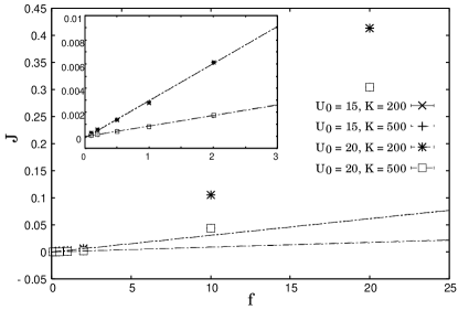
Figure 1: Current $J$ in the $x_{1}$ direction as a function of $f$. The average values of $J$ for 10 samples are plotted for several values of $f$. The statistical error bars are smaller than the symbols. Inset: Close-up of the linear response regime.

Now, we study the statistical properties of the density field

$$\rho({\boldsymbol{x}},t)=\sum_{i=1}^{N}\delta({\boldsymbol{x}}-{\boldsymbol{x}}_{i}(t)).$$ (6)

We consider the Fourier series of the density field

$$\hat{\rho}_{(n_{1},n_{2})}= \int d^{2}{\boldsymbol{x}}\rho({\boldsymbol{x}})e^{-i\frac{2\pi}{L}(n_{1}x_{1}+n_{2}x_{2})}.$$ (7)

Using this, we characterize density fluctuations on large scales in terms of the correlation coefficient

$$C\equiv\left\langle\left({\rm Re}[\delta\hat{\rho}_{(0,1)}]\right)^{2}\right\rangle,$$ (8)

where $\delta\hat{\rho}_{(n_{1},n_{2})}$ is a Fourier series of the deviation $\delta\rho({\boldsymbol{x}})=\rho({\boldsymbol{x}})-\left\langle\rho({\boldsymbol{x}})\right\rangle$ from the average density profile $\left\langle\rho({\boldsymbol{x}})\right\rangle$, and ${\rm Re}[\ ]$ represents the real part of a complex number.

According to the fluctuation-response relation, which is valid in equilibrium cases, $C$ is related to a response coefficient against a potential perturbation. In the present problem, we consider the response of ${\rm Re}[\delta\hat{\rho}_{(0,1)}]$ to the potential

$$V({\boldsymbol{x}})=\epsilon\cos\left(\frac{2\pi x_{2}}{L}\right).$$ (9)

We note that this potential does not depend on $x_{1}$, that is, we apply the perturbation potential transversal to the external field $f$ in a manner similar to that in Refs. HS1 ; SST . Quantitatively, the response coefficient is defined as

$$R\equiv-\lim_{\epsilon\rightarrow 0}\frac{\left\langle{\rm Re}[\delta\hat{\rho}_{(0,1)}]\right\rangle_{\epsilon}}{\epsilon},$$ (10)

where $\left\langle\ \right\rangle_{\epsilon}$ represents the statistical average in the steady state under the potential (9).

Here, by the fluctuation-response relation is meant

$$C=TR.$$ (11)

Although it should hold in equilibrium cases, there is no reason to expect that it also holds in non-equilibrium systems. Nevertheless, we can measure both $C$ and $R$ even for non-equilibrium systems. Thus, we can check the relation concretely by numerical experiments.

III conjecture

Before presenting the results of numerical experiments, we review the understanding of the relation given in Eq. (11). In equilibrium cases, the relation can be directly obtained from the canonical distribution; however, here we present an alternative, phenomenological understanding based on a macroscopic fluctuation theory in order to consider an extension of the relation.

Let $\tilde{\rho}({\boldsymbol{x}})$ be a fluctuating density field defined at a macroscopic scale. Then, due to the large deviation property, the stationary distribution is written as

$$P_{\rm S}(\tilde{\rho}(\cdot))\simeq\exp\left(-L^{2}I(\tilde{\rho}(\cdot))\right),$$ (12)

where $I(\tilde{\rho}(\cdot))$ is called a large deviation functional. According to the fluctuation theory for systems under equilibrium conditions, $I$ is determined by thermodynamics. Concretely, using a free energy density $f(T,\rho)$, we can write

$$I(\tilde{\rho}(\cdot))=\frac{1}{TL^{2}}\int d^{2}{\boldsymbol{x}} [f(T,\tilde{\rho}({\boldsymbol{x}}))-f(T,\bar{\rho})$$

$$+V({\boldsymbol{x}})(\tilde{\rho}({\boldsymbol{x}})-\bar{\rho})],$$ (13)

where $\bar{\rho}$ is the average density. This relation is called Einstein’s formula and can be proved within a framework of equilibrium statistical mechanics. Noting that $\hat{\rho}_{(0,1)}$ is an example of macroscopic density fluctuations, we find that Eq. (11) is obtained from Eqs. (12) and (13).

Equations (12) and (13) are so simple that they are expected to be extended to those valid in non-equilibrium systems. More concretely, we conjecture that Eq. (13) holds if the free energy is extended in a consistent manner.

In this conjecture, the existence of the extended free energy is highly nontrivial. Indeed, severe restrictions are required to construct thermodynamics in non-equilibrium steady states, as discussed in Ref. SST . Nevertheless, we already know that thermodynamics can be extended in non-equilibrium states for driven lattice gases when we focus on the transversal direction to the driving force HS1 ; SST . Since the present model has common features with driven lattice gases, we expect that the thermodynamics can be extended to our model in a manner similar to that for driven lattice gases.

These considerations lead us to conjecture the validity of Eq. (11), although the statistical distribution is not canonical in non-equilibrium cases. Note that Eq. (11) can be checked independently of the question whether or not thermodynamic functions can be extended to non-equilibrium steady states.

IV Measurement and result

Before measuring $C$ and $R$, we estimate the relaxation time $\tau_{\rm D}$ for the density field. This estimation is necessary for the accurate determination of statistical averages by numerical experiments. Since perturbation effects of the potential $V({\boldsymbol{x}})$ can be neglected, we estimate $\tau_{\rm D}$ only for the systems without this potential. Initially, we prepare an inhomogeneous particle configuration; as an example, all particles are placed on the sites of a hexagonal lattice with the lattice interval $2r_{c}$. Then, we observe a diffusion phenomenon of the density field by solving Eq. (1) numerically. Because we found that the diffusion in the $x_{1}$ direction is slower than that in the $x_{2}$ direction, we measure only the time dependence of $\hat{\rho}_{(1,0)}(t)$. Repeating this procedure $30$ times, we estimate the statistical average of $|\hat{\rho}_{(1,0)}(t)|$. We then obtain a fitting $|\hat{\rho}_{(1,0)}(t)|=|\hat{\rho}_{(1,0)}(0)|e^{-t/\tau_{\rm D}}$. We found that the $K$ dependence of $\tau_{\rm D}$ is small and that $\tau_{\rm D}$ is a decreasing function of $f$ when the other parameters are fixed. From these observations, we estimate $\tau_{\rm D}$ for the system with $U_{0}$, $K$, and $f$ by measuring $\tau_{\rm D}$ for the system with $f=0$, $K=200$, and $V({\boldsymbol{x}})=0$.

Using $\tau_{\rm D}$ evaluated above, we estimate a statistical average $\left\langle A\right\rangle_{\epsilon}$ using a time average

$$\left\langle A\right\rangle_{\epsilon}=\frac{1}{\tau}\int_{t_{0}}^{t_{0}+\tau}dtA(t),$$ (14)

where we chose the values of $t_{0}$ and $\tau$ as those more than 40 times of the relaxation time $\tau_{\rm D}$ for the density field.

We now measure $R$ in Eq. (10) for all the values of $U_{0}$ and $K$ (mentioned previously) both under the equilibrium condition $f=0$ and the non-equilibrium condition $f=20$. By measuring $\left\langle{\rm Re}[\delta\hat{\rho}_{(0,1)}]\right\rangle_{\epsilon}$ for several values of $\epsilon$, we estimate the regime where it linearly depends on $\epsilon$. The slope in this region yields $R$. As one example, in Fig. 2, $\left\langle{\rm Re}[\delta\hat{\rho}_{(0,1)}]\right\rangle_{\epsilon}$ is displayed for $U_{0}=15$ and $K=200$: $R$ is evaluated as $5.51\pm 0.01$ for the non-equilibrium case ($f=20$), while it is $4.64\pm 0.03$ for the equilibrium case.

Figure 2: Average values of $\left\langle{\rm Re}[\delta\hat{\rho}_{(0,1)}]\right\rangle_{\epsilon}$ over $100$ samples are plotted as a function of $\epsilon$. $U_{0}=15$ and $K=200$. The statistical error bars are smaller than the symbols.

Next, we measure $C=\langle({\rm Re}[\delta\hat{\rho}_{(0,1)}])^{2}\rangle_{0}$ for the same values of the parameters. We find that for $f=20$, the value of $C$ shows clear deviation from the equilibrium value. This suggests that the stationary distribution of $\rho$ in the non-equilibrium case is not close to the equilibrium distribution.

From the two independent measurements of $R$ and $C$, we can check the fluctuation-response relation $C=TR$. The result is summarized in Fig 3. This suggests that the relation given in Eq. (11) holds even in the non-equilibrium steady states to a similar extent as that in the equilibrium states.

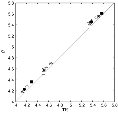
Figure 3: $C$ vs $TR$ for several values of $U_{0},K$, and $f$. Two same symbols correspond to the data obtained by using the same $U_{0}$ and $K$ for the equilibrium and non-equilibrium conditions.

Here, we present a remark on the systematic deviation from the equality in Fig 3. Let us recall that the validity of the equality given in Eq. (11) can be proved mathematically in equilibrium cases. Therefore, each point in Fig. 3 should exist on the solid line within the statistical error bar at least for the equilibrium cases. We conjecture that the slight but systematic deviation from the solid line in Fig. 3 is caused by numerical inaccuracy associated with a choice of the value of $\Delta t$. In order to check it further, we measured how the deviation depends on the time step $\Delta t$ in our numerical calculation. As shown in Fig 4, $C/(RT)$ approaches 1 in the limit $\Delta t\to 0$. Thus, we expect that in both equilibrium and non-equilibrium cases, the fluctuation-response relation holds with a higher accuracy if we perform numerical experiments with a smaller $\Delta t$.

Figure 4: $(C-TR)/TR$ as a function of the time step $\Delta t$. $U_{0}=15$ and $K=200$.

V concluding remarks

Before concluding this paper, we present two remarks. First, let us notice that the system we study is a typical example of the so-called driven diffusive system Schmidttmann ; Gregory ; Garrido . It has been believed that in such a system the equal-time spatial correlation function generally exhibits a power-law decay of the type $r^{-d}$ for a large distance $r$, where $d$ is the spatial dimension of the system Grinstein ; Dorfman . This power-low decay is called the long-range correlation. In fact, it has been proved for the model given in Eq. (1) that this type of long-range correlation appears when the interaction length between two particles is sufficiently larger than the period $\ell$ NakamuraSasa . However, such a nonlocal behavior of density fluctuations was not observed in our numerical experiments. A plausible explanation for this apparent inconsistency might be that the system size we study is much smaller than that at which the long-range correlation can be observed, though the system size is so large that thermodynamic fluctuations can be argued. Further studies will be necessary in order to gain a clearer understanding.

As the second remark, we address an example of laboratory experimental systems related to our study and consider the possibility of observing our simulation results experimentally. First, since a periodic potential with a period of $6$ $\mu$m can be designed by using an optical instrument Brunner , let us assume that $\ell=1$ corresponds to $6\mu$m. Then $r_{c}=2.0$ and $L=30$ correspond to $12.0$ $\mu$m and $180$ $\mu$m, respectively. Here, the cutoff radius $r_{c}$ may be interpreted as an interaction range such as the Debye screening length of the screened Coulomb potential. According to Ref. Blaaderen , such a long screening length can be realized experimentally. Note that the core radius of the particle is of the order of micrometers. Next, in order to realize the periodic boundary conditions in the direction of the external force, it might be a good method to place all the particles under a rotating optical tweezer with a velocity $v$ Seifert . Indeed, by observing the system in the moving frame $v$, we can confirm that the spatially homogeneous force $f=\gamma v$ is produced with periodic boundary conditions. (See Fig. 5.) We expect that such an implementation is possible due to the recent development of the optical technology Grier2 .

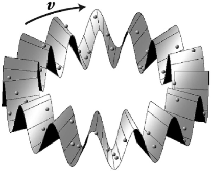
Figure 5: Schematic figure of a driven diffusive system under periodic boundary conditions.

In conclusion, we have demonstrated that the fluctuation-response relation given in Eq. (11) is plausible for many Brownian particles under an external driving force when we focus on a direction transversal to the driving force. If this relation is valid for any average density, one can obtain a formula that relates the intensity of density fluctuations in the transversal direction to the derivative of a chemical potential with respect to the density HS1 . Then, by measuring the work required to change the system size in the transversal direction, one may confirm the Maxwell relation, which ensures the existence of a thermodynamic function extended to non-equilibrium steady states SST ; HS1 . In this manner, we will confirm Einstein’s formula for the system we study. This provides a realistic and nontrivial example for a framework of steady-state thermodynamics.

We thank Masaki Sano, Yoshihiro Murayama, and Kumiko Hayashi for their helpful suggestions. This work was supported by a grant (No. 19540394) from the Ministry of Education, Science, Sports and Culture of Japan.

References

-
(1)
Electronic address:
takenobu.nakamura@aist.go.jp
- (2) R. Kubo, M. Toda, and N. Hashitsume, Statistical Physics II: Nonequilibrium Statistical Mechanics (Springer, Berlin, 1991).
- (3) K. Hayashi and S.I. Sasa, Phys. Rev. E 68, 035104(R), (2003).
- (4) S. Sasa and H. Tasaki, J. Stat. Phys. 125, 125, (2006).
- (5) B. Derrida, J. L. Lebowitz, and E. R. Speer, Phys. Rev. Lett. 87, 150601, (2001); B. Derrida, J. L. Lebowitz, and E. R. Speer, J. Stat. Phys. 107, 599, (2002).
- (6) B. Derrida, J. L. Lebowitz, and E. R. Speer, Phys. Rev. Lett. 89, 030601, (2002); B. Derrida, J. L. Lebowitz, and E. R. Speer, J. Stat. Phys. 110, 775, (2003).
- (7) P. T. Korda, M. B. Taylor, and D. G. Grier, Phys. Rev. Lett. 89, 128301, (2002).
- (8) J. C. Crocker and D. G. Grier, Phys. Rev. Lett. 73, 352, (1994).
- (9) P. T. Korda, G. C. Spalding, and D. G. Grier, Phys. Rev. B 66, 024504, (2002).
- (10) V. Blickle, T. Speck, C. Lutz, U. Seifert, and C. Bechinger, Phys. Rev. Lett. 98, 210601, (2007).
- (11) B. Schimttmann and R. K. P. Zia, Statistical mechanics of driven diffusive systems (Academic Press, 1995).
- (12) G. L. Eyink, J. L. Lebowitz, and H. Spohn, J. Stat. Phys. 83, 385, (1996).
- (13) P. L. Garrido, J. L. Lebowitz, C. Maes, and H. Spohn, Phys. Rev. A 42, 1954, (1990).
- (14) G. Grinstein, D. H. Lee and S. Sachdev, Phys. Rev. Lett. 64, 1927, (1990).
- (15) J. R. Dorfman, T. R. Kirkpatrick, and J. V. Sengers, Ann. Rev. Phys. Chem. 45, 213, (1994).
- (16) T. Nakamura and S.I. Sasa, Phys. Rev. E 74, 031105, (2006).
- (17) C. Bechinger, M. Brunner, and P. Leiderer, Phys. Rev. Lett. 86, 930, (2001).
- (18) A. Yethiraj and A. v. Blaaderen, Nature 421, 513, (2003).