Morphology of flows and buoyant bubbles in the Virgo cluster

Abstract

There is growing evidence that the active galactic nuclei (AGN) associated with the central elliptical galaxy in clusters of galaxies are playing an important role in the evolution of the intracluster medium (ICM) and clusters themselves. We use high resolution three-dimensional simulations to study the interaction of the cavities created by AGN outflows (bubbles) with the ambient ICM. The gravitational potential of the cluster is modelled using the observed temperature and density profiles of the Virgo cluster. We demonstrate the importance of the hydrodynamical Kutta-Zhukovsky forces associated with the vortex ring structure of the bubbles, and discuss possible effects of diffusive processes on their evolution.

1 Introduction

It has been more then 40 years since the first detection of x-ray emission from a cluster of galaxies was made. The emission was detected from around the M87 galaxy (Byram et al., 1966) at the centre of the Virgo cluster, whose proximity helped to get high resolution maps of the x-ray emitting gas (Matsushita et al., 2002; Young et al., 2002; Ghizzardi et al., 2004, hereafter G04). Later observations revealed that many clusters are bright x-ray sources, with luminosities in the range $10^{43\ldots 45}$$\,\textup{erg\,s}^{-1}$. The properties of the x-ray emission from clusters of galaxies were found to be most consistent with thermal bremsstrahlung from hot gas (Sarazin, 1986). This implies that the observed ICM has an electron density, $n_{\text{e}}$, in the range of $10^{-4\ldots-2}\,{\rm cm}^{-3}$, and a temperature, $T_{\text{a}}$, of the order $10^{7\ldots 8}$ K.

The radiative cooling time of the gas in a cluster core due to bremsstrahlung can be as short as $10^{6}$ yr. Unless the gas is thermally supported, the cooling leads inexorably to an inflow of the cold gas onto the central galaxy (for a review of cooling flow theory see, e.g., Fabian, 1994). However, many observations have since demonstrated both the lack of the cold gas deposits, and spectroscopically determined mass deposition rates up to an order of magnitude smaller than the rates predicted by the classical cooling flow model (Voigt & Fabian, 2004).

This apparent contradiction has led to the suggestion that the gas in the cluster cores is reheated. A number of different mechanisms were proposed to reduce the cooling flow (or prevent it from forming in the first place): currently the most popular candidates are outflows from active galactic nuclei (AGN) (see, e.g., Churazov et al., 2001; Brüggen & Kaiser, 2002; Bîrzan et al., 2004); thermal conduction of heat from the outer regions (see, e.g., Narayan & Medvedev, 2001; Voigt et al., 2002; Voigt & Fabian, 2004; Pope et al., 2006); disruption and heating of the flow by sound waves and turbulence (see, e.g., Ruszkowski et al., 2004; Fujita & Suzuki, 2005; Fujita et al., 2004); heating by supernovae explosions (see, e.g., Voit & Bryan, 2001; Pipino et al., 2002; Tang & Wang, 2005). Clear discrimination between the different models based on the observational data is difficult. Morphological features of the x-ray emission were used as the evidence in favour of a particular mechanism (Ruszkowski et al., 2004; Fabian et al., 2003; Brüggen et al., 2005). The morphological resemblance is important, and although it is impossible to base a prove in favour of a particular mechanism on the morphology alone, it is important to understand how different physical processes affect the morphology of the observed features.

Despite some recent progress in the understanding of the physical state of the ICM (Enßlin et al., 2005; Enßlin & Vogt, 2006; Lazarian, 2006), many key parameters remain not well known. Since laboratory experiments on plasma with conditions close to those found in astronomical objects are still rare (Keenan & Rose, 2004), all estimates of such physical properties of the ICM as the values of thermal diffusivity and viscosity are generally based on modifications of the values calculated in the classical work of Spitzer (1962). It is accepted that magnetic fields decrease the diffusivity, since they suppress movements of charged particles across the field lines. The same is believed to be true for the value of the viscosity as well. Usually a fraction of the Spitzer value is used to approximate thermal diffusivity of the ICM (Chandran & Cowley, 1998; Narayan & Medvedev, 2001), which assumes chaotic orientation of the magnetic field lines (i.e., magnetic fields lines are bent on scales smaller than the mean free path of an electron in the plasma). The value of the thermal conductivity in turbulent ICM can be an order of magnitude larger than the Spitzer value, as shown by Cho et al. (2003) and Lazarian (2006). The exact extent of this amplification depends on the state of the turbulence in the ICM, which is difficult to estimate from the present observational data.

The kinetic effects are likely to be important in the context of the ICM physics. Collisionless interactions on the scale smaller than the mean free path can affect the overall dynamics of the AGN-ICM interaction (Schekochihin et al., 2006, 2005).

1.1 The Model

While a model that accounts for the above mentioned physical properties of the ICM is clearly necessary for a detailed understanding of its dynamics, we will use a simplified approach in order to investigate certain aspects of the dynamics related to AGN activity. In this work we use a purely hydrodynamical model of the ICM, which includes radiative cooling to simulate conditions preexisting to AGN activity due to the cooling flow.

We use numerical simulations to study the morphology of the AGN-blown bubbles. We do not simulate inflation of the bubbles by AGN outflows, instead we introduce them as perturbations of the temperature and density fields of the cluster at a certain point during the simulation (see §2.3 for more details). While the inflation of the bubbles can influence their subsequent evolution, we are more interested in the time scales that are larger than the inflation time, and the effects of numerical techniques on the hydrodynamics of the bubbles. Although the effect of the velocity field produced by the jet inflation of the bubbles is likely to be important especially during the early stages of the evolution, here we study the influence of the velocity field induced by the buoyantly rising bubble and the fluid instabilities developing on its surface on the morphology of the bubbles. The combined effect of the jet injection and buoyancy will be addressed in the future work.

The gravitational potential of the cluster is modelled using observed temperature and density profiles for the Virgo cluster as determined by G04, using XMM, BeppoSAX and Chandra data (see §2.2 for more details). The observational data allows for more accurate modelling of the gravitational potential then a fitted theoretical profile (e.g., NFW, Navarro et al., 1997), as the gravity of the central galaxy can become dominant at the cluster core.

The outline of the current work is as follows: in § 2 we discuss numerical framework and initial conditions for our simulations, in § 3 we present analysis of the simulations. In § 4 we discuss implications and limitations of the current work. Finally, we present our main conclusions in § 5.

2 Numerical Framework

For our numerical experiment we use flash (version 2.3) – a modular, adaptive-mesh (AMR), parallel simulation code, capable of handling general compressible flow problems found in many astrophysical environments (Fryxell et al., 2000).

The hydro module of the flash code solves Euler’s equations in three dimensions. In the conservative form the equations are given by,

$$\frac{\partial\rho}{\partial t}+\nabla\cdot\left(\rho\mathbf{v}\right)=0,$$ (1)

$$\frac{\partial\rho\mathbf{v}}{\partial t}+\nabla\cdot\left(\rho\mathbf{v}\otimes\mathbf{v}\right)+\nabla P=\rho\mathbf{g}$$ (2)

$$\frac{\partial\rho{\cal E}}{\partial t}+\nabla\cdot\left(\left(\rho{\cal E}+P\right)\mathbf{v}\right)=\rho\left(\mathbf{v}\cdot\mathbf{g}\right)$$ (3)

where $\rho$ is the fluid density, $\mathbf{v}$ is the fluid velocity, $P$ is the pressure, ${\cal E}$ is the sum of the internal energy $E$, and the kinetic energy per unit mass, ${\cal E}=E+|\mathbf{v}|^{2}/2$, $\Lambda$ is the cooling function (see § 2.1), and $(\mathbf{v}\otimes\mathbf{v})_{ij}=v_{i}v_{j}$ denotes a tensor product.

The physical size of the computational grid is $10^{24}\,{\rm cm}\approx 322$ kpc in each direction. Numerically the grid is constructed using nested blocks of $16^{3}$ cells, with the ratio of sizes between the neighbouring blocks being either 1:1 or 1:2. The minimum refinement level (minimum level of nested blocks with 1:2 ratio) is set to 3, which results in the largest cell size of $10^{24}\,{\rm cm}/(2^{3-1}16)=10^{24}\,{\rm cm}/64\approx 1.56\times 10^{22}\,{\rm cm}\approx 5$ kpc. The maximum refinement level was set to 8, giving a minimum cell size of $10^{24}\,{\rm cm}/(2^{8-1}16)=10^{24}\,{\rm cm}/2048\approx 4.88\times 10^{20}\,{\rm cm}\approx 0.16$ kpc.

2.1 Radiative Cooling

We have developed a new module for flash, which implements the cooling function, $\Lambda$ (see Fig. 1), to account for the radiative losses from the fully ionised plasma in the wide range of temperatures, $4<\log T<8.5$, using the values tabulated by Sutherland & Dopita (1993) (metallicity was taken to equal half solar [Fe/H]$=-0.5$). For temperatures exceeding $\log T=8.5$ we calculate $\Lambda$ using the formula for thermal bremsstrahlung (McKee & Cowie, 1977),

$$\dot{E}=-\frac{1}{\rho}\Lambda,$$ (4)

$$\Lambda=n_{\text{e}}n_{\text{p}}\Lambda_{\text{N}},$$ (5)

$$\Lambda_{\text{N}}=2.5\times 10^{-27}T^{0.5}\quad\text{[erg s${}^{-1}$ cm${}^{3}$]},$$ (6)

where $\dot{E}$ is the rate of the energy loss per unit mass, $n_{\text{e}}$, $n_{\text{p}}$ are the electron and proton number densities, which for fully ionised gas with primordial abundances (mass of Helium is 0.25 of total mass of the gas) relates to the mass density of the ICM as,

$$n_{\text{e}}=1.167n_{\text{p}},$$ (7)

$$\rho=1.143n_{\text{e}}a,$$ (8)

where $a=1.661\times 10^{-24}$ g is the atomic mass unit ($\approx m_{\text{p}}$).

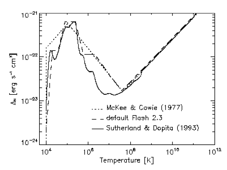
Figure 1: Dependence of the cooling function, $\Lambda_{\text{N}}$, on temperature (see § 2.1): thick line – the current model; dashed line – the original flash cooling function; dotted line – the cooling function from McKee & Cowie (1977).

The new cooling function accounts for line cooling in much greater detail, but it does not differ significantly from the default flash module (source_terms/cool/radloss), see Fig. 1. The only serious departure from the default approximation occurs around temperature of $T\sim 10^{7}$ K, were the original module overestimates the energy loss by a factor of a few ($\sim 5$). It is important to note, that in our simulations most of the gas has temperatures within this range, and therefore this difference is non-negligible. The radiative losses were not applied to the gas with temperatures below $T=10^{4}$ K because the present scheme does not thermally resolve gas at such temperatures (cooling length becomes smaller than the numerical resolution of our grid).

2.2 Initial Conditions

We model the cluster gravitational potential using the data from G04. Using the de-projected temperature and electron number density profiles of the Virgo cluster,

$$T(x)=T_{1}-T_{2}\exp\{-x^{2}/(2x_{2}^{2})\},$$ (9)

$$n_{\text{e}}(x)=n_{1}\left(1+(x/x_{1})^{2}\right)^{-a_{1}}+n_{2}\left(1+(x/x_{2})^{2}\right)^{-a_{2}},$$ (10)

where $x_{1}=1.54\times 10^{22}\,{\rm cm}=5$ kpc, $x_{2}=7.19\times 10^{22}\,{\rm cm}=23.3$ kpc, $a_{1}=1.518$, $a_{2}=0.705$, $T_{1}=2.78\times 10^{7}$ K, and $T_{2}=8.997\times 10^{6}$ K, $n_{1}=0.089\,{\rm cm}^{-3}$, $n_{2}=0.019\,{\rm cm}^{-3}$, (see Fig. 2), we compute the gravitational acceleration due to the cluster’s gravitational potential from the assumption of hydrostatic equilibrium (HSE),

$$\frac{1}{\rho}\frac{{\rm d}P}{{\rm d}x}=g(x),$$

where $P=nk_{\text{B}}T$ is the thermal pressure, and $g(x)$ is the gravitational acceleration.

At the beginning of the simulations we set the temperature field to be uniform, $T_{0}=3\times 10^{7}$ K, and the initial density distribution is determined from the requirement of HSE. Since HSE fixes only the gradient of the density, we are left to choose the peak density, $\rho_{0}$, ad hoc. From a number of one dimensional test simulations (without AGN heating) we determined the optimal value as $\rho_{0}=5.15\times 10^{26}$ g cm^-3, which provides the best fit to the observational profiles on the outskirts of the cluster at time $t\sim 10^{10}$ yr after the beginning of the simulation (see also simulations by Pope et al., 2005).

Figure 2: Left panel: observed temperature and density profiles of the Virgo cluster from G04. The lines are the analytical fit, see equations (9) and (10). Right panel: gravitational acceleration as a function of distance from the centre, derived from HSE conditions using the best-fit lines.

2.3 Introduction of Bubbles

We use a single fluid in flash to represent both ambient ICM and the gas inside bubbles, unlike the two-fluid approach used by Brüggen et al. (2005) and Ruszkowski et al. (2004). The bubbles are introduced into the simulation when the temperature of a computational cell in the vicinity of the centre falls below $T=1.5$ keV. This trigger temperature serves as a simple feedback mechanism that relates cooling flow parameters to the heating response. The value $1.5$ keV was selected to be close to the observed temperature minimum, see Fig. 2.

The temperature field perturbations associated with the bubbles are introduced using a modified version of the perturbation module util/perturb, which is supplied with flash. We position the centres of the perturbations symmetrically on opposite sides of the centre of the grid (cluster), at distances of $x_{0}=1.5r_{0}=1.5\times 10^{22}\,{\rm cm}=4.86$ kpc, with randomly specified orientation angles of the line connecting the bubbles and the cluster centre. The locations for the bubbles are refined up to the maximum refinement level prior to the introduction of the bubbles.

The temperature of all computational cells with coordinates $\mathbf{b}$, satisfying the inequality $r_{0}\leq|\mathbf{b}-\mathbf{c}_{i}|$, where $\mathbf{c}_{i}$ ($i=1,2$) are the position-vectors of the bubble centres, is modified using the following algorithm. Each computational cell $\mathbf{b}$ is sub-divided into $4\times 4\times 4$ sub-cells ($\mathbf{b}_{s}$, $s=1,\ldots,64$). The temperature of each sub-cell is set to $T_{\text{b}}=5\times 10^{10}$ K if $r_{0}<|\mathbf{b}_{s}-\mathbf{c}_{i}|$, and is left unchanged otherwise. The temperature of a computational cell is then calculated as a volume average of temperatures of its sub-cells, $T(\mathbf{b})=1/64\sum_{s}^{64}T(\mathbf{b}_{s})$. This algorithm provided a sharp transition boundary between the bubble and the ICM (so-called top-hat perturbation profile), but is sufficiently robust not to cause any numerical difficulties.

To make the temperature perturbations thermodynamically consistent, we choose a pressure profile, and calculate the corresponding densities using the equation of state for an ideal gas. We tested two profiles: the pressure inside the bubble matches the pressure of the ambient medium (i.e. the pressure field is not changed by the perturbation), and a constant pressure profile, where the value of the constant pressure is calculated as a volume average of the pressure field inside the perturbation region before the introduction of the bubbles. However, we find that since the sound speed inside the bubble is much higher than the sound speed of the ambient medium, in the former case the pressure inside the bubble quickly reaches a constant profile, sending a weak sound wave into the ICM. In order to avoid this additional artificial disturbance we used constant pressure profiles in our setup. Further analysis (see § 3) showed that the difference in the initial conditions does not lead to a serious discrepancy in the properties of the bubbles. The minor effects caused by it will be discussed in § 4. As a first order approximation, however, the difference between the parameters of the bubbles in these two cases can be viewed as an intrinsic scatter caused by our numerical scheme.

3 Simulation Results

In this section we present an analysis of the data from simulations with two kinds of the initial pressure profiles for bubbles, model a has the initial pressure profile matching the ambient pressure and c has the initial constant pressure profile.

The core of the cluster met the criterion for injection of bubbles after $t=706$ Myr, so the bubbles are introduced into an established cooling flow. At this stage the ambient temperature of the ICM at the distance $x_{0}=1.5r_{0}$ from the centre is $T(x_{0})\approx 2.62\times 10^{7}$ K, density $\rho(x_{0})\approx 2.83\times 10^{-26}$ g cm^-3, and the cooling time $\Delta t\approx 1.7$ Gyr. Due to the large cooling time we can ignore the effects of the radiative cooling on the parameters of the bubbles.

In our purely hydrodynamical simulations we need to resolve the smallest scales of the instabilities in order to account properly for the small scale mixing of the hot gas with the ambient ICM. The key parameter in the stabilisation of the bubble/ambient medium interface against the RT instability is the surface tension, which can be provided by the magnetic field lines parallel to the surface of the bubble. As it was shown by Kaiser et al. (2005) (hereafter K05) and De Young (2003) even weak magnetic surface tension (magnetic fields of $\sim 0.1\mu$G) stabilise the bubble surface on scales up to 0.1 kpc at the distance of $5$ kpc from the centre of the cluster (see Fig. 3, K05). By limiting the smallest cell size to $h=0.16$ kpc we essentially assume that the gas will be fully mixed on the scale $\sim h$ on the time scale of $h/c_{\text{s}}~{}\sim 10^{13}$ s, which is approximately equal to the growth time of the RT instability of the scale $h$ in the absence of viscosity (see Fig. 2, K05). Although a fully consistent model should include magnetic fields to account for the stabilisation of the bubble surface (Ruszkowski et al., 2007), these simple estimates show that the numerical resolution of our model is consistent with the expected dynamics of the system, as follows from the analytical stability analysis, and numerical simulations with ‘random’ magnetic fields.

3.1 Bubble Surface

As the bubbles ascent in the ICM their shape and position changes. In order to study their parameters we have used a simple technique for identification of the material inside bubbles at any stage during their evolution. Firstly, we note that the averaged radial entropy index ($\sigma=\rho^{-2/3}T$) profile for the ICM, can be well fitted with a linear function, $\langle\sigma\rangle=\sigma_{\text{a}}x+\sigma_{\text{b}}$, where $x$ is a distance from the centre, at any time during the simulations in both models. Secondly, by constructing the entropy profile using the means over large enough spherical shells (i.e., using low resolution profiling) we can abate the contribution from the high entropy regions associated with the bubbles ($V_{\text{bubble}}/V_{\text{shell}}\ll 1$). The variances of the values of $\sigma$ in each shell are used as an error estimate for the values of the means in the fitting routine, which further reduces influence of the high entropy bubbles on the result of the linear fitting. We mark as “bubble” any computational cell with an entropy index above $1.5(\sigma_{\text{a}}x+\sigma_{\text{b}})$, where $x$ is the distance of the cell to the centre of the cluster (grid), and $\sigma_{\text{a,b}}$ are the fitted coefficients for the current time.

The surface of the bubbles becomes irregular due to RT instabilities, and small bits of the bubble are shredded away as it rises through the ICM and fragments. In such circumstances a measure of the size and position of the bubble material has to be essentially statistical, and not just purely geometrical.

To quantify the size of the bubble we measure its extension in the direction of ascent, $R_{||}$, and its size in the direction perpendicular to the direction of ascent, $R_{\bot}$. For a purely spherical bubble $R_{||}=R_{\bot}$. When the bubble has the shape of a torus we measure both external and internal radii of the torus, $R_{\bot(\text{max,min})}=\max,\min(R_{\bot})$, using the following algorithm. The position vector of a “bubble” cell, $\mathbf{R}_{i}$, is split into the component aligned with the direction specified by a vector connecting the centre of the cluster and the initial position of the bubble, $\mathbf{R}_{||i}$ (the direction of ascent), and the vector perpendicular to the first one, going through the centre of the cell, $\mathbf{R}_{\bot i}$, so that, $\mathbf{R}_{i}=\mathbf{R}_{||i}+\mathbf{R}_{\bot i}$. We then compute histograms (using 100 bins) of $|\mathbf{R}_{\bot i}|$ and $|\mathbf{R}_{||i}|$, using the values of the corresponding vectors $\mathbf{R_{(||,\bot)i}}$ for all cells of a single bubble. We use the cut off at the level of 0.1 of the maxima of the histogram to find the approximate extent of the bubble material (and exclude any trailing and overtaking bits; we select the bins below the cut-off which are closest to the peak of the histogram), that gives the inner and outer radii of the torus, $R_{\bot\text{max,min}}$, or, in the case of the ’quasi-spherical’ bubble, two measures of the radius, $R_{\bot}=R_{\bot\text{max}}$, and $R_{||}=0.5(R_{||\text{max}}-R_{||\text{min}})$. The means of the $|R_{(||,\bot)i}|$ with the exclusion of the values below the cut-off, correspond to the distance of the bubble from the centre of the cluster (in the case of $|\mathbf{R}_{||i}|$), and a mean radius of the torus (in the case of $|\mathbf{R}_{\bot i}|$).

3.2 Morphology

The surfaces of bubbles rising in the ICM corrugates due to Reilegh-Taylor (RT) instability, however, this does not result in an immediate dispersion of the bubbles, see Fig. 7. In fact, the mass diffusion due to the RT instability and numerical diffusion remains quite small and the bubbles in simulations a and c remain traceable for a long time. We can still find traces of the old bubble material after the second pair of bubbles was injected ($>100$ Myr).

We find that during the ascent the size of the bubbles does not change adiabatically according with the change of the ambient pressure with distance from the centre of the cluster,

$$V(x)=V_{0}(P(x)/P_{0})^{-1/\gamma},$$ (11)

where $P(x)$ is the pressure profile, with $\gamma=5/3$. Also the velocity of the bubbles does not reach a terminal level, as it is usually expected from a simple theoretical analysis (see, e.g., Enßlin & Heinz, 2002).

As shown in Fig. 3, the volume of the bubbles keeps growing after the injection and then it plateaus. The growth of the volume of the bubble (which is identified as the region of high entropy) is the consequence of several different processes. One of them is the adiabatic expansion due to the pressure change with distance from the centre of the cluster as given by equation (11), another one is the entrainment of ambient plasma through the surface of the bubble (mixing), and the third one is the enlargement of the bubble due to the hydrodynamical Kutta-Zhukovsky forces as explained below. Full quantitative description of the evolution of the bubble parameters is out of scope of this work, and is addressed in the follow-up article (Pavlovski et al., 2007).

In our numerical experiment the entrainment of the ICM through the boundary of the bubble is a consequence of the instabilities that develop on the surface of the bubbles (see Fig. 7), and, unavoidably, the numerical diffusion. In reality the diffusion of the plasma across the boundary of the bubble is controlled by the magnetic field, and the resulting change of the volume of the bubble is likely to be different both from the prediction given by equation (11), and the results of our numerical model. It is important to note, however, that any amount of mixing will lead to violation of the adiabatic assumption. Unless the mixing process is understood in greater detail, and other adiabatic processes like Kutta-Zhukovsky forces are taken into account, the estimate of the AGN energy input from the estimates of the total volume of the bubbles is likely to be inaccurate.

The initial growth of the volume of the bubbles corresponds to the deceleration phase in their ascent, which follows the very sharp initial acceleration, see Fig. 4. The slight re-acceleration of the bubbles at $x\approx 3r_{0}$ corresponds to the change of the morphology of the bubbles from spherical to toroidal, after which the bubbles continue to decelerate. As explained below, the velocity of the bubble is tightly linked with the increase in its volume by a simple physical mechanism.

Figure 3: Change of the volume of bubbles with height. Note that due to discretisation (finite resolution of the grid) and the algorithm we use for identification of the bubble cells during the analysis, the initial volume of the bubble is less than the geometrical value $V_{0}=4/3\pi r_{0}^{3}$. The dash-dotted line shows the predicted isotropic adiabatic expansion of the spherical bubble according to equation (11). The initial volume is taken to be equal to the initial volume of bubble determined by the bubble finding algorithm.

Figure 4: Change of the ascent velocity of the bubbles with height.

The initial expansion of the bubble is not isotropic, see Figs. 5 and 6. The volume of a bubble increases due to the sideways expansion (expansion in the direction perpendicular to the direction of ascent, $\bot$-direction), whereas the size of the bubbles in the direction of the ascent ($||$-direction) stays roughly constant. The ellipticity of the bubbles, $e=\sqrt{1-(R_{||}/R_{\bot})^{2}}$, quickly reaches saturation at a level of $e\approx 0.9$ in both cases.

Figure 5: Change of the size of the bubbles in the direction of the ascent ($||$-direction), and the ellipticity, $\sqrt{1-(R_{||}/R_{\bot})^{2}}$, of the bubbles.

Figure 6: Change of the size of the bubbles in the direction perpendicular to the direction of ascent ($\bot$-direction).

The flattening of the bubbles can not be attributed to the viscosity, since no physical viscosity is modelled. In presence of viscous stresses they would act to squeeze the bubble in the $||$-direction. They would result in an increase of pressure inside the bubble, which would act to restore the equilibrium. This process can result in oscillations of the surface of the bubble (by analogy with oscillations of the buoyant bubbles in a lava lamp), but is unlikely to lead to any net increase in their volume.

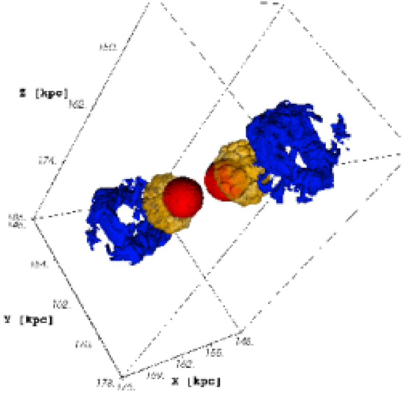
Figure 7: Surfaces of the bubbles. The bubbles closest to the centre correspond to the time of the injection and are spherically symmetric. The later stages correspond to times 18 Myr and 98 Myr after the injection for (model c). Note the ‘finger-like’ corrugation of the surfaces of the bubbles.

3.3 Kutta-Zhukovsky forces

The structure of the flow through the bubble has the geometry of a vortex ring right from the very early stages, when the bubble is still roughly spherical, see Fig. 8. This circumstance has a profound effect on the evolution of the bubble.

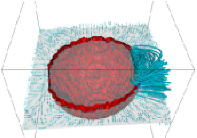
Figure 8: The flow around the spherical bubble shows the structure of a vortex ring. The visualisation shows part of the surface of the bubble (the upper half is cut off) in simulation c, 2.3 Myr after the injection. The arrows show the direction of the velocity in a thin slab just below the cut plane. The tubes trace the stream lines close to the centre of the right vortex on the cut plane.

As a hot bubble starts to ascend, it can retain its spherical shape only if the fluid motion inside the bubble correspond to a perfect fluid dipole (by analogy with so-called Hill’s solution, see, e.g., Saffman, 1995). If during the ascent the spherical symmetry breaks down (i.e., $R_{\bot}$ becomes larger than $R_{||}$), the fluid motion inside the bubble corresponds to the circulation around a stretched dipole – the vortex ring.

In the beginning we can consider the inner radius of the vortex ring (torus) to be equal to zero (the bubble is roughly spherical), and the velocity of ascent to be equal to the maximum ascent velocity, see Fig. 4. Due to drag the speed of the ascent and of the vortex flow will decrease. Since the vortex moves with respect to the ambient medium each element of the vortex is subject to the Kutta-Zhukovsky force (for an introduction to aerodynamic forces see, e.g., Landau & Lifshitz (1987) § 38, and appendix A), which acts to expand the vortex radially. This force acts to expand the bubble in the $\bot$-direction, eventually creating a hole in the middle of the bubble – the bubble becomes torus shaped. As the vortex ring expands radially, an additional component of the Kutta-Zhukovsky force pushes the bubble down, reducing its ascent velocity. Indeed, with rapid vortex expansion the total velocity vector of the elements of the vortex ring will no longer be aligned in the $||$-direction, but will have a component in the $\bot$-direction as well, see Fig. 9. This results in the Kutta-Zhukovsky force pointing down in the $||$-direction, in the direction opposite to the velocity of ascent. This force will act to reduce the velocity of the ascent, i.e., it counteracts buoyancy.

Figure 9: The forces acting on an element of the vortex ring: $F_{\text{b}}$ - buoyancy, $F_{\text{d}}$ - drag, $F_{\text{kz}}$ - Kutta-Zhukovsky force. Dashed arrows show the components of the velocity: the ascent velocity $U=\dot{x}$ and the expansion velocity $u=\dot{R}$.

Let $R=\langle R_{||}\rangle$ be the radius of the torus, and $r$ the radius of its cross-section, see Fig. 9. If $\alpha$ is the central angle, so that $R\text{d}\alpha$ is the length of an element of the vortex ring, then this element will be subject to a Kutta-Zhukovsky force,

$$\Gamma U^{\prime}\rho_{\text{a}}\left(1+\left(\frac{\dot{R}}{U^{\prime}}\right)^{2}\right)^{1/2}R\text{d}\alpha,$$ (12)

where $\dot{R}=\text{d}R/\text{d}t$ is the speed of the vortex expansion, $\Gamma$ is the vortex circulation (see appendix A), $\rho_{\text{a}}$ is the density of the ICM, and $U^{\prime}=U-v^{\prime}$, $U$ is the ascent velocity, $v^{\prime}$ is the self-induced (vertical) velocity of the vortex (Batchelor, 1967),

$$v^{\prime}\approx\frac{\Gamma}{4\pi R}\log\frac{R}{r}.$$ (13)

The Kutta-Zhukovsky force points at an angle $\beta$ to the $\bot$-direction,

$$\begin{split}\sin\beta=\frac{\dot{R}/U^{\prime}}{\sqrt{1+\left(\dot{R}/U^{\prime}\right)^{2}}},\\ \cos\beta=\frac{1}{\sqrt{1+\left(\dot{R}/U^{\prime}\right)^{2}}}.\\ \end{split}$$ (14)

So, the vertical component of the Kutta-Zhukovsky force, acting on the whole vortex ring is,

$$F_{||\text{kz}}=2\pi R\Gamma\dot{R}\rho_{\text{a}}.$$ (15)

Figure 10: Change of the ratio of the magnitude of the $||$-component of the Kutta-Zhukovsky force to the magnitude of the buoyant force.

In Fig. 10 we plot the ratio of the vertical component of the Kutta-Zhukovsky force to the buoyant force acting on the bubbles as a function of their distance from the cluster centre. To estimate the circulation of the vortex we calculated the mass-weighted mean of the velocity of the bubble material in the rest frame of the bubble. This is clearly just an estimate, and the resulting plot has some scatter as a result. It does, however, illustrate the main points discussed above, and shows that the magnitude of the Kutta-Zhukovsky force is comparable to the buoyant force. A quantitative model of the evolution of the bubbles is out of the scope of this work (see Pavlovski et al., 2007, for more details).

4 Discussion

In the present work we have omitted the phase during which the jets inflate the bubbles, which limits applicability of this model to the interpretation of observations. However, the dynamics of the flow around bubbles created by a jet is likely to be similar, once the bubbles become buoyant. Taking the jet injection into account it is quite possible that the vortex ring structure will form much earlier (during the injection) and the flow around the bubble will have a larger initial value of circulation, $\Gamma$, which can be induced by the viscous momentum transfer of the kinetic energy of the jet, as suggested by the laboratory experiments of small scale jets (see, e.g., Afanasyev, 2006). Kutta-Zhukovsky forces are then likely to be even more important for the dynamics and the overall energy balance.

The parameters of the bubbles with different initial pressure profiles (models a and c) do not differ greatly, see Figs. 3 – 6. The only noticeable difference is that the bubbles in simulation a develop a comparatively large secondary torus. This secondary vortex ring (torus) is shredded from the main vortex soon after the bubbles morph into tori, it separates from the much bigger main torus, and travels in front of it. The volume of this secondary torus is small compared to the volume of the bubble, and its contribution to the size of the bubble was discarded (it has generally fallen below the 10 per cent cut-off, see § 3.1) during the calculations. The secondary vortex ring quickly mixes with the ambient ICM and dissipates. The fact that this vortex ring has a larger volume in case a is reflected in the evolution of the total volume of the bubbles, see Fig. 3. The volume of the a-bubbles is getting smaller than the volume of the c-bubbles once their secondary tori mix with the ICM. It also results in a slightly smaller $R_{\bot}$ size of the a-bubbles at later stages of the evolution, see Fig. 6.

4.1 The role of missing physics

High temperature plasma in the absence of the magnetic fields is thought to be thermally conductive and viscous (Spitzer, 1962). The diffusivity coefficients are sensitive functions of temperature, $\propto T^{2.5}$. This ensures that any temperature gradient on scales larger than the mean free path of an electron is smoothed out very efficiently by the conduction, and fluid instabilities are damped by the viscosity (Kaiser et al., 2005).

We have attempted to simulate the dynamics of bubbles in a viscous and thermally conductive ICM. Our experiments showed, however, that unless thermal conduction is very efficiently suppressed on the boundary of the bubble, it leads to a very fast erosion of the bubble material (although no fluid instabilities develop). This is easy to understand from the following simple estimate. Given that the amount of heat in the bubble is of the order $\Delta Q\sim pV\approx 10^{55}$ erg, the difference in the temperatures of the plasma inside the bubble and the ambient ICM $\Delta T\sim T\approx 10^{9}$ K, the coefficient of the thermal conductivity for plasma at $T=10^{7}$ K is $\kappa\sim 10^{11}$ erg s^-1 cm^-1 K^-1, then the timescale of the evaporation of the bubble is $\Delta t=\Delta Q\Delta l/(\kappa\Delta TS)\sim 1$ Myr, where we let $\Delta l\sim R$, and $S\sim R^{2}$. Therefore it is not at all surprising that we found that the bubbles were fully mixed with ICM at a distance of $\sim 3\ldots 4r_{0}$ from the centre of the cluster. Without the inclusion of magnetic fields into the numerical model it is impossible to draw a definitive conclusion about the evolution of the bubbles in a diffusive ICM. Magnetic field draping (Ruszkowski et al., 2007) is likely to play a significant role in the dispersion of the bubbles in thermally conductive ICM.

We note, however, that the above discussion of the KZ forces does still remain valid even in our ‘superdiffusive’ cases (see appendix B for further details), i.e. the bubbles still morph into tori, and the vortex motion is present.

The morphology of the observed bubbles in the Perseus cluster was used as an indicator of a possible highly viscous ICM in (Reynolds et al., 2005). We would argue, however, that the flattening of the bubble, which was explained by Reynolds et al. (2005) as a result of viscosity, has an additional explanation. It is the Kutta-Zhukovsky forces, not viscosity, that determine the radial size of the bubbles, and it is impossible to infer the importance of viscous effects in the ICM from the morphology of the bubbles alone. Viscosity acts to suppress RT instabilities but does not prevent morphing of the initially spherical bubbles into tori. At this stage the presence of a significant viscosity in galaxy clusters should be regarded as speculative, unless directly confirmed by observations.

5 Conclusions

In the present work we have used a numerical scheme based on the flash code to produce three dimensional simulations of AGN bubble heating of the ICM, with an emphasis on the dynamics of the bubbles. Our setup includes a sophisticated cooling function to help establish the initial cooling flow, followed by the introduction of the high contrast AGN-bubbles, which dynamics we have analysed.

The data presented in this article are consistent with the results of previous numerical simulations of the AGN bubble heating of the ICM (Gardini, 2007; Reynolds et al., 2005; Brüggen & Kaiser, 2002). However, our analysis has indicated additional important phenomena linked to the dynamics of the gas of the bubbles in the ICM. Our main results are as follows.

1. Bubbles change shape and transform into tori not because of hydrodynamical instabilities, but due to the radial Kutta-Zhukovsky force.

2. Bubbles do not reach a terminal velocity defined by the balance between the drag force and the buoyancy. The velocity of their ascent is also affected by the the vertical Kutta-Zhukovsky force and the self-induced velocity of the vortex.

3. Viscosity does play a role in stabilising the surface of the bubbles against instabilities, but it does not alter their overall 3D (torus-like) morphology.

4. The volume of bubbles can lead to an erroneous estimation of the energy supplied by the AGN when using equation (11). The expansion of the bubbles is not only due the change of the ambient pressure but also due to the Kutta-Zhukovsky forces, and non-adiabatic turbulent mixing. A more accurate model of plasma (including magnetic fields) is needed in order to make realistic prediction about the entrainment of the ICM into the bubbles.

5. Thermal conduction must be highly suppressed on the boundary of the bubbles, otherwise it leads to a rapid erosion (mixing) of the bubble material.

A better knowledge of the physical state of the ICM is of paramount importance for further progress in understanding the interaction of AGN outflows with the ICM.

6 Acknowledgements

This research has made use of NASA’s Astrophysics Data System Bibliographic Services. The software used in this work was in part developed by the DOE-supported ASC / Alliance Center for Astrophysical Thermonuclear flashes at the University of Chicago. We would like to thank flash developers Tomasz Plewa and Timur Linde for prompt response to our questions. GP and CRK thank PPARC for financial support.

Appendix A Nature of the Kutta-Zhukovsky forces

Circulation is the line integral around a closed curve of the fluid velocity. If $\mathbf{v}$ is the fluid velocity and d$\mathbf{s}$ is a unit vector along the closed curve $C$, the circulation is given by,

$$\Gamma=\oint_{C}\mathbf{v}\cdot\text{d}\mathbf{s}.$$

The units of circulation are [cm² s^-1]. The Kutta-Zhukovsky theorem states that the lift force acting per unit span on a body in an inviscid flow field can be expressed as the product of the circulation about the body, $\Gamma$, the fluid density, $\rho$, and the speed of the body relative to the free-stream, $U$,

$$f=U\rho\Gamma.$$

This equation applies both around airfoils, where the circulation is generated by airfoil action, and around spinning objects, experiencing the Magnus effect, where the circulation is induced mechanically. The latter case is governed by the same basic principles as apply to the travelling vortices. A spinning object (e.g., a cylinder rotating around its axis of symmetry, or an eddy) creates a motion of the fluid in the boundary layer around it (e.g., via viscous drag) – the circulation. If such a rotating object travels through the fluid (e.g., the rotating cylinder travels through the fluid at rest in the laboratory frame of reference, with its axis of symmetry remaining parallel to itself), on one side of it, the velocity of the fluid in the boundary layer will be in the same direction as the velocity of the surrounding fluid near it. On this side the resulting velocity of the fluid will be larger than the travel velocity. On the other side of the object, the velocity of the fluid in the boundary layer will be in the opposite direction of the velocity of the fluid near it, and the resulting velocity of the fluid will be smaller than the travel velocity. According to the Bernoulli’s theorem the quantity $p+v^{2}/2=$ const along flow lines, so the pressure $p$ will be lower on one side of the rotating cylinder than on the other causing an unbalanced force at a right angle to the travel velocity.

Appendix B Numerical experiments with thermal conductivity

In order to account for the suppression of the diffusive processes in the presence of chaotic magnetic fields the diffusive coefficients for conductivity, $\kappa_{\text{s}}$, and viscosity, $\eta_{\text{s}}$, are reduced by a certain factor, $0\leq f_{\text{s}}\leq 1$. In the case of AGN blown bubbles this suppression is likely to be much stronger inside the bubbles (due to the associated strong magnetic field), resulting in the suppression coefficient being not spatially uniform,

$$\kappa=f_{\text{s}}(\mathbf{x})\kappa_{\text{s}},$$ (16)

$$\eta=f_{\text{s}}(\mathbf{x})\eta_{s},$$ (17)

$$f_{\text{s}}(\mathbf{x})=\begin{cases}f_{\text{s}1},&\text{outside bubbles},\\ f_{\text{s}2},&\text{inside bubbles}.\end{cases}$$ (18)

The factor $f_{\text{s}1}$ is a simulation parameter. We have tested a range of possible values: $f_{\text{s}1}=[0.1,0.3,0.6]$. In order to identify the computational cells that are located inside the bubbles and to apply a different suppression factor to them, we probe cells inside the spherical central region of the size $x_{7}=7r_{0}=7\times 10^{22}\,{\rm cm}=22.7$ kpc, where $r_{0}$ is the initial radius of the bubbles, and $x_{7}=7r_{0}$ is an estimate of the maximum height the bubbles are likely to reach, starting at the distance of $1.5r_{0}$ from the centre of the cluster (see also § 2.3). At each time-step we compare the entropy index, $\sigma=T\rho^{-2/3}$, of the cells inside the $|\mathbf{x}|<x_{7}$ region with the cutoff value, $\sigma_{7}$. The cutoff value is computed for each time-step as, $\sigma_{7}=1.5\langle\sigma\rangle_{x_{7}<|\mathbf{x}|\leq x_{7}+\Delta x}$, which is 1.5 times the average of the entropy index in a spherical shell with radius $x_{7}$, and thickness $\Delta x=0.5r_{0}=5\times 10^{21}\,{\rm cm}=1.6$ kpc. We then define $f_{s2}$ as,

$$f_{\text{s}2}=\begin{cases}5.\times 10^{-12}\left(\frac{2\sigma_{7}}{3\sigma}\right)^{1.5},&\text{if}\,\sigma>\sigma_{7},\\ f_{\text{s}1},&\text{otherwise},\end{cases}$$ (19)

where the factor $\left(2\sigma_{7}/3\sigma\right)^{1.5}\approx(T_{\text{a}}/T_{\text{b}})^{2.5}$ accounts for the increase of the conductivity and viscosity coefficients due to the large temperature of the bubbles, $T_{\text{b}}$, compared to the temperature of the ambient gas, $T_{\text{a}}$. This scheme is designed to effectively suppress diffusive process inside the bubbles. It could not, however, prevent diffusion of the bubble material and its mixing with the ICM.

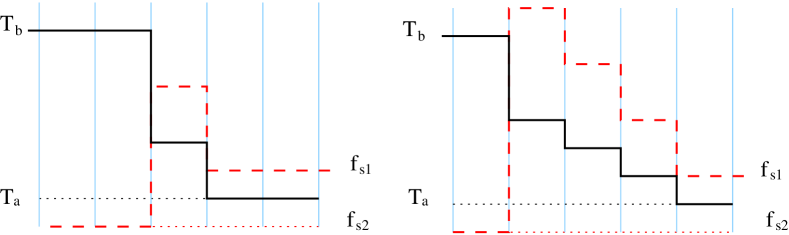
Figure 11: Schematic of the growth of a conductive layer around the bubble due to the discretization of the temperature gradient. The vertical lines represent boundaries of the computational cells. The solid line represents the temperature profile at the edge of the bubble, where $T_{\text{b}}$ is the temperature of the gas inside the bubble, and $T_{\text{a}}$ is the temperature of the ambient medium. The dashed line represents the corresponding value of the thermal conduction. The suppression coefficient $f_{\text{s}1}$ is applied to the gas at temperature $T_{\text{a}}$, and $f_{\text{s}2}$ to the gas at temperature $T_{\text{b}}$ . The panel on the left represents the initial profiles. Thermal conduction works to reduce the temperature gradient, and creates a number of cells with an intermediate values of temperatures (entropies) and high conductivities (right panel).

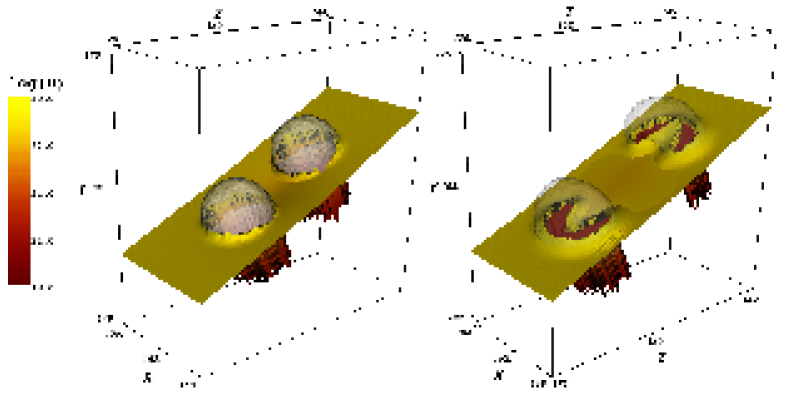
Figure 12: Growth of a conductive layer around the bubbles in a 3D simulation. The visualisation shows surface cuts through the scalar field equal to the logarithm of the thermal diffusivity. The resulting surfaces are colour-coded and warped according to the value of the scalar. Semi-transparent surfaces show the edge of the bubbles. The data are taken from the simulation with $f_{\text{s1}}=0.1$: on the moment of injection (left), 8 Myr later (right). The size of the box is given in kiloparsecs.

In our diffusive simulations discretization of the temperature gradient leads to formation of a layer of thermally conductive plasma around the bubble, as illustrated in Figs. 11 and 12. This layer is essentially an artifact of our numerical scheme for the suppression of the diffusive processes, and is not reflective of the real physical properties of the ICM.

The problem with discretization is going to be present in the two-fluid approach as well (by two-fluid approach we mean separate fluids for the bubble and the ambient medium as used by, e.g., Brüggen et al. (2005)). We believe it will lead to a qualitatively similar behaviour, since the suppression coefficient for the diffusion in this case is also based on an ad hoc cut off based on the concentration of the bubble fluid in a computational cell.

Without a more advanced model, which needs to include magnetic fields, and self-consistently accounts for the suppression of the diffusive processes, it is impossible to say whether or not this is a realistic representation of the real state of the ICM.

We find that the dynamics and morphology of the bubbles in our diffusive simulations also governed by KZ forces, since the circulative flow around the bubble is always present.

References

- Afanasyev (2006) Afanasyev Y. D., 2006, Physics of Fluids, 18, 037103
- Batchelor (1967) Batchelor G. K., 1967, An introduction to fluid dynamics. Cambridge University Press
- Bîrzan et al. (2004) Bîrzan L., Rafferty D. A., McNamara B. R., Wise M. W., Nulsen P. E. J., 2004, ApJ, 607, 800
- Brüggen & Kaiser (2002) Brüggen M., Kaiser C. R., 2002, Nat., 418, 301
- Brüggen et al. (2005) Brüggen M., Ruszkowski M., Hallman E., 2005, ApJ, 630, 740
- Byram et al. (1966) Byram E. T., Chubb T. A., Friedman H., 1966, Science, 152, 66
- Chandran & Cowley (1998) Chandran B. D. G., Cowley S. C., 1998, Physical Review Letters, 80, 3077
- Cho et al. (2003) Cho J., Lazarian A., Honein A., Knaepen B., Kassinos S., Moin P., 2003, ApJ, 589, L77
- Churazov et al. (2001) Churazov E., Brüggen M., Kaiser C. R., Böhringer H., Forman W., 2001, ApJ, 554, 261
- De Young (2003) De Young D. S., 2003, MNRAS, 343, 719
- Enßlin & Heinz (2002) Enßlin T. A., Heinz S., 2002, A&A, 384, L27
- Enßlin & Vogt (2006) Enßlin T. A., Vogt C., 2006, A&A, 453, 447
- Enßlin et al. (2005) Enßlin T. A., Vogt C., C. Pfrommer 2005, in ’The Magnetized Plasma in Galaxy Evolution’ Krakow, Poland, Sept. 27th - Oct. 1st, 2004 Magnetic Fields in Clusters of Galaxies. p. 231
- Fabian (1994) Fabian A. C., 1994, ARA&A, 32, 277
- Fabian et al. (2003) Fabian A. C., Sanders J. S., Crawford C. S., Conselice C. J., Gallagher J. S., Wyse R. F. G., 2003, MNRAS, 344, L48
- Fraenkel (1972) Fraenkel L. E., 1972, J. Fluid Mech., 51, 119
- Fryxell et al. (2000) Fryxell B., Olson K., Ricker P., Timmes F. X., Zingale M., Lamb D. Q., MacNeice P., Rosner R., Truran J. W., Tufo H., 2000, ApJS, 131, 273
- Fujita et al. (2004) Fujita Y., Matsumoto T., Wada K., 2004, Journal of Korean Astronomical Society, 37, 571
- Fujita & Suzuki (2005) Fujita Y., Suzuki T. K., 2005, ApJ, 630, L1
- Gardini (2007) Gardini A., 2007, A&A, 464, 143
- Ghizzardi et al. (2004) Ghizzardi S., Molendi S., Pizzolato F., De Grandi S., 2004, ApJ, 609, 638
- Kaiser et al. (2005) Kaiser C. R., Pavlovski G., Pope E. C. D., Fangohr H., 2005, MNRAS, 359, 493
- Keenan & Rose (2004) Keenan F. P., Rose S. J., 2004, Astronomy and Geophysics, 45, 18
- Landau & Lifshitz (1987) Landau L. D., Lifshitz E. M., 1987, Fluid Mechanics, second edn. Vol. 4, Pergamon Press
- Lazarian (2006) Lazarian A., 2006, ApJ, 645, L25
- Matsushita et al. (2002) Matsushita K., Belsole E., Finoguenov A., Böhringer H., 2002, A&A, 386, 77
- McKee & Cowie (1977) McKee C. F., Cowie L. L., 1977, ApJ, 215, 213
- Morton (1960) Morton B. R., 1960, J. Fluid Mech., 9, 107
- Narayan & Medvedev (2001) Narayan R., Medvedev M. V., 2001, ApJ, 562, L129
- Navarro et al. (1997) Navarro J. F., Frenk C. S., White S. D. M., 1997, ApJ, 490, 493
- Pavlovski et al. (2007) Pavlovski G., Kaiser C. R., Pope E. C. D., 2007, Dynamics of buoyant bubbles in clusters of galaxies, submitted, arXiv:0709.1796
- Pipino et al. (2002) Pipino A., Matteucci F., Borgani S., Biviano A., 2002, New Astronomy, 7, 227
- Pope et al. (2005) Pope E. C. D., Pavlovski G., Kaiser C. R., Fangohr H., 2005, MNRAS, 364, 13
- Pope et al. (2006) Pope E. C. D., Pavlovski G., Kaiser C. R., Fangohr H., 2006, MNRAS, 367, 1121
- Reynolds et al. (2005) Reynolds C. S., McKernan B., Fabian A. C., Stone J. M., Vernaleo J. C., 2005, MNRAS, 357, 242
- Ruszkowski et al. (2004) Ruszkowski M., Brüggen M., Begelman M. C., 2004, ApJ, 615, 675
- Ruszkowski et al. (2007) Ruszkowski M., Enßlin T. A., Brüggen M., Heinz S., Pfrommer C., 2007, MNRAS, pp 400–+
- Saffman (1995) Saffman P. G., 1995, Vortex Dynamics, second edn. Cambridge University Press
- Sarazin (1986) Sarazin C. L., 1986, Reviews of Modern Physics, 58, 1
- Schekochihin et al. (2006) Schekochihin A. A., Cowley S. C., Dorland W., 2006, ArXiv Astrophysics e-prints
- Schekochihin et al. (2005) Schekochihin A. A., Cowley S. C., Kulsrud R. M., Hammett G. W., Sharma P., 2005, in ’The Magnetized Plasma in Galaxy Evolution’ Krakow, Poland, Sept. 27th - Oct. 1st, 2004 Magnetised plasma turbulence in clusters of galaxies. p. 200
- Spitzer (1962) Spitzer L., 1962, Physics of Fully Ionized Gases. Inerscience, New York
- Sutherland & Dopita (1993) Sutherland R. S., Dopita M. A., 1993, ApJS, 88, 253
- Tang & Wang (2005) Tang S., Wang Q. D., 2005, ApJ, 628, 205
- Turner (1957) Turner J. S., 1957, Proc. Roy. Soc. A., 239, 61
- Turner (1969) Turner J. S., 1969, Annu. Rev. Fluid Mech., 1, 29
- Voigt & Fabian (2004) Voigt L. M., Fabian A. C., 2004, MNRAS, 347, 1130
- Voigt et al. (2002) Voigt L. M., Schmidt R. W., Fabian A. C., Allen S. W., Johnstone R. M., 2002, MNRAS, 335, L7
- Voit & Bryan (2001) Voit G. M., Bryan G. L., 2001, Nat., 414, 425
- Young et al. (2002) Young A. J., Wilson A. S., Mundell C. G., 2002, ApJ, 579, 560