We present a complete 1-loop study of the electroweak corrections to the process $ug\to dW^{+}$ in MSSM and SM. The occurrence of a number of remarkable properties in the behavior of the helicity amplitudes at high energies is stressed, and the crucial role of the virtual SUSY contributions in establishing them, is emphasized. The approach to asymptopia of these amplitudes is discussed, comparing the effects of the logarithmic and constant contributions to the mass suppressed ones, which are relevant at lower energies. Applying crossing to $ug\to dW^{+}$, we obtain all subprocesses needed for the 1-loop electroweak corrections to $W^{\pm}$-production at LHC. The SUSY model dependence of such a production is then studied, and illustrations are given for the transverse $W^{\pm}$ momentum distribution, as well as the angular distribution in the subprocess center of mass.

PACS numbers: 12.15.-y, 12.15.-Lk, 14.70.Fm, 14.80.Ly

1 Introduction

The general properties of the virtual supersymmetric (SUSY) electroweak corrections to the amplitude of any process at high energies have already been identified in the literature [1]. In particular, precise rules for all logarithmic contributions have been established, completing those applying to the Standard Model (SM) case [2]. These rules provide simple and clear asymptotic tests of the SUSY gauge and Yukawa couplings, and several applications have been given for $e^{-}e^{+}$ and hadron colliders.

Moreover it has been shown in [3], that for any gauge supersymmetric theory, the helicity amplitudes $F_{\lambda_{a}\lambda_{b}\lambda_{c}\lambda_{d}}$ for any two-body processes

$$a_{\lambda_{a}}+b_{\lambda_{b}}\to c_{\lambda_{c}}+d_{\lambda_{d}}~{}~{},$$ (1)

at fixed angles and very high energies, must satisfy conservation of total helicity. Here $(a,b,c,d)$ denote fermions, gauge bosons or scalar particles, and $(\lambda_{a},\lambda_{b},...)$ describe their helicities. This means that at energies much higher than all masses in the theory, only the helicity amplitudes obeying

$$\lambda_{a}+\lambda_{b}=\lambda_{c}+\lambda_{d}~{},$$ (2)

may acquire non-vanishing values. The validity of (2), to all orders in any softly broken supersymmetric extension of SM, like e.g. MSSM, is referred to as the Helicity Conservation (HC) rule, and its general proof has been presented in [3].

In the non supersymmetric standard model (SM), HC is also approximately correct, to 1-loop leading logarithmic accuracy. In such a case, where all particles in (1) are assumed to be ordinary SM ones, the asymptotically dominant amplitudes should also obey (2); but the subdominant ones, which violate (2), should asymptotically tend to (possibly non-vanishing) constants.

As emphasized in [3], the validity of the HC rule is particularly tricky when some of the participating particles are gauge bosons; because then large cancellations among the various diagrams are needed for establishing it. Moreover, the general proof is based on neglecting all masses and the electroweak breaking scale, at asymptotic energies [3]. It is therefore interesting to check the HC validity at specific complete 1-loop calculations, in order to be sure that no asymptotically non-vanishing terms, involving e.g. ratio of masses, violate it.

Such an example is given by the process $ug\to dW^{+}$ considered here. When neglecting the light quark masses for this process, $u$ and $d$ quarks always carry negative helicities, so that the helicity conservation property (2), effectively refers only to the helicities of the incoming $g$ and outgoing $W$. Thus for $ug\to dW^{+}$, the asymptotically dominant amplitudes determined by HC actually are

$$F_{\lambda_{u}\lambda_{g}\lambda_{d}\lambda_{W}}=F_{----}~{},~{}F_{-+-+}~{},$$ (3)

which we call gauge boson helicity conserving (GBHC) amplitudes.

The first purpose of the present paper is to explore how such high energy and fixed angle properties for the helicity amplitudes are generated in an exact one-loop electroweak computation, in either SM or MSSM; and how these asymptotic features are corrected at lower energies by sub-leading contributions.

Having achieved this, the second purpose is to look at the electroweak corrections to $W^{\pm}$+ jet production at the large high energy hadron collider LHC. Provided infrared effects are appropriately factored out, the relevant subprocesses are $qg\to q^{\prime}W$, $\bar{q}g\to\bar{q}^{\prime}W$ and $q\bar{q}^{\prime}\to Wg$ [4].

For such processes, QCD corrections have been carefully considered since a long time in [5], and more recently for the case of the large transverse momentum distribution [6]. Electroweak corrections to the $W^{\pm}$ transverse momentum $p_{T}$ distribution in SM, have been recently discussed by Kühn et al. [7] and by Hollik at al [8], where infrared corrections have also been included, which necessitates considering the direct photon emission, in addition to $W$+jet production.

At high $p_{T}$ at LHC, the SM electroweak corrections turn out to be large, due to the occurrence of single and quadratic logarithmic effects, as expected from the aforementioned asymptotic rules [2]. In the studies of [7, 8] though, no attention had been paid to the behavior of the specific helicity amplitudes and the SUSY contribution to them.

Consequently, as already mentioned, these are the aspects, on which we concentrate in the present paper. In more detail, we study how the complete one loop results for the various $ug\to dW^{+}$ helicity amplitudes match at high energy with the asymptotic rules established in [1, 3], thus assessing the importance of the subleading terms at LHC energies.

The outcome is that supersymmetry indeed plays a crucial role in establishing the gauge boson helicity conservation. Particularly for the gauge boson helicity violating (GBHV) amplitudes

$$F_{---+}~{},~{}F_{---0}~{},~{}F_{-+--}~{},~{}F_{-+-0}~{},$$ (4)

which violate (2), it is striking to see how the cancellation between the standard and supersymmetric loop contributions is realized, enforcing the vanishing the GBHV amplitudes at high energies. In other words, in a high energy expansion of these amplitudes in MSSM, not only the logarithmic terms cancel out, but also the tiny ”constant” contributions.

We add here that the $ug\to dW^{+}$ processes has been chosen because of its theoretical simplicity; not necessarily because of its best observability, or of its largest SUSY effects. It only constitutes a simple toy for studying the supersymmetric effects on the helicity amplitudes. The properties we find should be instructive and indicative of those expected for other types of processes accessible for hadron, lepton or photon colliders. We hope to undertake such studies in the future.

The contents of the next Sections is the following. In Sect. 2 we consider the basic $ug\to dW^{+}$ process, defining the kinematics and helicity amplitudes and classifying the various one loop diagrams. In Sect. 3 we present the detail behavior of the various GBHC and GBHV amplitudes at one loop in SM and MSSM. The importance of the various high energy components (leading logs, constant terms, mass-suppressed terms) and the role of SUSY, are discussed by considering several benchmark models of the constrained MSSM type.

Using then $ug\to dW^{+}$ and the processes related to it by crossing, as well as the appropriate parton distribution functions (PDF) [9], we present in Sect.4 the transverse momentum distribution for $W^{\pm}$ production in association with a jet at LHC. In addition to it, the $W^{\pm}$ angular distribution in the subprocess center of mass is also shown. The observability of these supersymmetry properties is briefly discussed. Finally, in Sect.5 we give our conclusions and suggest some further applications.

2 One loop electroweak amplitudes for $ug\to dW^{+}$.

The momenta and helicities in this process are defined by

$$u(p_{u},\lambda_{u})+g(p_{g},\lambda_{g})\to d(p_{d},\lambda_{d})+W^{+}(p_{W},\lambda_{W})~{}~{},$$ (5)

and the corresponding helicity amplitudes are denoted as $F_{\lambda_{u}\lambda_{g}\lambda_{d}\lambda_{W}}$. Neglecting the $(u,d)$-quark masses and remembering that the $W$-quark coupling is purely left-handed implying $\lambda_{u}=\lambda_{d}=-1/2$, while the gluon and $W$ helicities can be $(\lambda_{g}=\pm 1),~{}(\lambda_{W}=\pm 1,0)$, we end up with only 6 possibly non-vanishing helicity amplitudes, which are

$$F_{----}~{},~{}F_{-+-+}~{},~{}F_{---+}~{},~{}F_{---0}~{},~{}F_{-+--}~{},~{}F_{-+-0}~{}~{}.$$ (6)

As it has already been mentioned immediately after (3), the first two of these amplitudes satisfy the HC rule (2) and are called GBHC. The remaining amplitudes, which have already appeared in (4), are called GBHV. Since they violate HC, they must vanish asymptotically, and as will see below, they are usually very small, also for LHC energies. It is convenient for the discussion below to separate them in two pairs: namely $(F_{---+},F_{---0})$ referred to as GBHV1 amplitudes, and $(F_{-+--}~{},~{}F_{-+-0})$ referred to as GBHV2.

Defining the kinematical variables

$$s=(p_{g}+p_{u})^{2}=(p_{W}+p_{d})^{2}~{}~{},~{}~{}\beta^{\prime}=1-{m^{2}_{W}\over s}~{},$$

$$u=(p_{d}-p_{g})^{2}=(p_{u}-p_{W})^{2}=-{s\beta^{\prime}\over 2}(1+\cos\theta)~{},$$

$$t=(p_{g}-p_{W})^{2}=(p_{u}-p_{d})^{2}=-{s\beta^{\prime}\over 2}(1-\cos\theta)~{}~{},$$ (7)

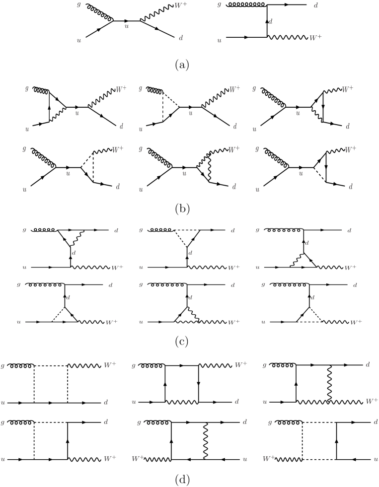
Figure 1: Independent Diagrams used for calculating the $ug\to dW$ helicity amplitudes. They consist of tree diagrams (a), s-channel 1-loop triangles (b), u-channel 1-loop triangles (c), and boxes (d). Full, broken and wavy lines describe respectively fermionic, scalar and gauge particles.

we first turn to the contribution of the Born diagrams in Fig.1a, containing u and d quark exchanges, in the s- and u-channel respectively. These affect the GBHC amplitudes $F_{----}$, $F_{-+-+}$, and the GBHV2 ones $F_{-+--}$, $F_{-+-0}$. For transverse ($\lambda_{W}=\pm 1$) and longitudinal ($\lambda_{W}=0$) $W^{+}$, these amplitudes are given respectively by

$$F^{\rm Born}_{-,\lambda_{g},-,\lambda_{W}} = \left(\frac{\lambda^{a}}{2}\right){eg_{s}\sqrt{\beta^{\prime}}\over 2\sqrt{2}s_{W}}\cos{\theta\over 2}\Bigg{\{}\Big{[}(1-\lambda_{g})(1-\lambda_{W})\Big{]}$$ (8)

$$+{1\over\beta^{\prime}}\Big{[}(1+\lambda_{g})(1+\lambda_{W})+{t\over u}\Big{(}1-\lambda_{g}(1-{2m^{2}_{W}\over s})\Big{)}(1-\lambda_{W})\Big{]}\Bigg{\}}~{},$$

$$F^{\rm Born}_{-,\lambda_{g},-,0} = \left(\frac{\lambda^{a}}{2}\right){eg_{s}\over 2m_{W}s_{W}}~{}\sin{\theta\over 2}\Bigg{\{}-\sqrt{s\beta^{\prime}}(1-\lambda_{g})+\frac{m_{W}^{2}(3\lambda_{g}+1)+s(1-\lambda_{g})}{\sqrt{s\beta^{\prime}}}\Bigg{\}}~{},$$ (9)

$$= \left(\frac{\lambda^{a}}{2}\right)\frac{eg_{s}}{s_{W}}\frac{m_{W}}{\sqrt{s\beta^{\prime}}}(1+\lambda_{g})\sin{\theta\over 2}~{}.$$

In (8, 9) the factor $\lambda^{a}/2$ describes the color matrices acting between the initial $u$ and final $d$ quark, while the first and second terms within the curly brackets come respectively from the s- and u-channel diagrams in Fig.1a.

We also note that since the amplitude $F_{-,\lambda_{g},-,0}$, given in (9), can never satisfy the HC rule (2), it has to vanish asymptotically, to any order in perturbation theory. The last expression in (9), is simply a tree order realization of this.

At the 1-loop level, the amplitudes in (8, 9) receive also contributions from the counter terms induced by the renormalization of the external particle fields and coupling constants, and determined by various gauge, $u$- and $d$-quark self energy diagrams. As input parameters in our renormalization scheme, we use the $W$ and $Z$ masses, through which the cosine of the Weinberg angle is also fixed; while the fine structure constant $\alpha$ is defined through the Thompson limit [10].

In SM, the aforementioned $u$- and $d$-quark self-energies are induced by the quark-gauge boson bubbles, while the Higgs and Goldstone bosons effects are negligible. The SM gauge self-energies come from gauge, Higgs and fermion loops.

Correspondingly, the main SUSY contribution to the quark self energies, consists of the squark-gaugino bubbles, while the additional SUSY Higgs bosons effects are again negligible. For the gauge self energies though, the SUSY contribution arises from gaugino, higgsino and sfermion loops, as well as the effects related to the two-doublet Higgs fields.

Including these counter term (c.t.) contributions to the above Born amplitudes, modifies them as

$$F^{\rm Born+c.t.}_{-,\lambda_{g},-,\lambda_{W}} = \left(\frac{\lambda^{a}}{2}\right){eg_{s}\sqrt{\beta^{\prime}}\over 2\sqrt{2}s_{W}}\cos{\theta\over 2}\Bigg{\{}\Big{[}(1+\delta_{s})(1-\lambda_{g})(1-\lambda_{W})\Big{]}$$ (10)

$$+{(1+\delta_{u})\over\beta^{\prime}}\Big{[}(1+\lambda_{g})(1+\lambda_{W})+{t\over u}\Big{(}1-\lambda_{g}(1-{2m^{2}_{W}\over s})\Big{)}(1-\lambda_{W})\Big{]}\Bigg{\}}~{},$$

$$F^{\rm Born+c.t.}_{-,\lambda_{g},-,0} = \left(\frac{\lambda^{a}}{2}\right){eg_{s}\over 2m_{W}s_{W}}~{}\sin{\theta\over 2}\Bigg{\{}-\sqrt{s\beta^{\prime}}(1-\lambda_{g})(1+\delta_{s})$$ (11)

$$+ \frac{m_{W}^{2}(3\lambda_{g}+1)+s(1-\lambda_{g})}{\sqrt{s\beta^{\prime}}}(1+\delta_{u})\Bigg{\}},$$

$$= \left(\frac{\lambda^{a}}{2}\right){eg_{s}m_{W}\over s_{W}\sqrt{s\beta^{\prime}}}~{}\sin{\theta\over 2}\Bigg{\{}(1+\lambda_{g})(1+\bar{\delta})$$

$$- \frac{\Sigma^{d}_{L}(u)(1+3\lambda_{g})}{2}-\frac{\Sigma^{u}_{L}(s)(1-\lambda_{g})}{2}+\frac{s(1-\lambda_{g})[\Sigma^{u}_{L}(s)-\Sigma^{d}_{L}(u)]}{2m_{W}^{2}}\Bigg{\}}~{},$$

where

$$\delta_{s}=\bar{\delta}-\Sigma^{u}_{L}(s)~{}~{},~{}~{}\delta_{u}=\bar{\delta}-\Sigma^{d}_{L}(u)~{}~{},$$ (12)

$$\bar{\delta}=\delta Z_{1}^{W}-\delta Z_{W}+{1\over 2}\delta\Psi_{W}+{1\over 2}\delta Z^{d}_{L}+{1\over 2}\delta Z^{u}_{L}~{}.$$ (13)

In (13), the first three terms in the r.h.s. come from the renormalization of the gauge couplings, masses and wave functions, through

$$\delta Z_{W}=-\Sigma^{T^{\prime}}_{\gamma\gamma}(0)+2{c_{W}\over s_{W}m^{2}_{Z}}\Sigma^{T}_{\gamma Z}(0)+{c^{2}_{W}\over s^{2}_{W}}\left[{\delta m^{2}_{Z}\over m^{2}_{Z}}-{\delta m^{2}_{W}\over m^{2}_{W}}\right]~{},$$

$$\delta m^{2}_{W}=Re\Sigma^{T}_{WW}(m^{2}_{W})~{}~{},~{}~{}\delta m^{2}_{Z}=Re\Sigma^{T}_{ZZ}(m^{2}_{Z})~{},$$

$$\delta Z_{1}^{W}-\delta Z_{W}={\Sigma^{T}_{\gamma Z}(0)\over s_{W}c_{W}M^{2}_{Z}}~{},~{}\Sigma^{T}_{\gamma Z}(0)=-\frac{\alpha}{2\pi}\frac{m_{W}^{2}}{s_{W}c_{W}}\left[\Delta-\ln\frac{m_{W}^{2}}{\mu^{2}}\right]~{},$$ (14)

$$\delta\Psi_{W}=-Re\hat{\Sigma}^{T^{\prime}}_{WW}(m^{2}_{W})=-\{Re\Sigma^{T^{\prime}}_{WW}(m^{2}_{W})+\delta Z_{W}\}~{}~{},$$ (15)

where $\Delta$ describes the usual ultraviolet contribution, in dimensional regularization. The needed gauge self energies in SM and SUSY may be found e.g. in the appendices of [11], expressed in terms of Passarino-Veltman (PV) functions [12].

Since, as discussed below, the infrared divergencies are always regularized by a non-vanishing ”photon mass” $m_{\gamma}$, this ”photon mass” must be inserted into the various $B_{j}$ functions taken from [11]. In addition to this, the quantity $\frac{\alpha}{2\pi}m_{\gamma}^{2}\Delta$ must be added to the r.h.s. of the expression (C.18) of [11].

We also note that the last two terms in the r.h.s of (13), as well as (12), come from the external quark wave functions and the self energies of the intermediate quarks in Fig.1a. These can also be obtained from the appendices of [11].

Finally, the validity of the HC rule for the amplitude (11), ensures that the last term within its curly brackets, which depends on quark self energies, must be cancelled at high energies, by some triangular and box contributions.

Having finished with the c.t. contributions to $ug\to dW^{+}$, we now turn to the triangular and box contributions from Fig.1.

The topologies of the triangular graphs consist of the left and right s-channel triangles appearing in Fig.1b, and the up and down u-channel triangles shown Fig.1c. The full, broken and wavy lines in this figure, describe respectively the various fermionic, scalar and gauge particles in SM or MSSM. We have checked explicitly that the ultraviolet divergences contained in these graphs, cancel exactly those induced by the counter terms in (10, 11).

The boxes for $ug\to dW$ are indicated in Fig.1d. The first two boxes are direct boxes, the next two boxes are the crossed ones, and the final two are the twisted boxes. All possible gauge, fermion and scalar exchanges should be taken into account, in both SM and MSSM.

Using (10, 11) and the triangular and box graphs mentioned above, we express the complete 1-loop electroweak amplitudes for $ug\to dW^{+}$ in the form

$$F^{\rm 1-loop}=\left(\frac{\lambda^{a}}{2}\right)\sum_{i=1}^{10}N_{i}(s,t,u)~{}\bar{u}_{d}K_{i}P_{L}u_{u}~{},$$ (16)

where the factor $\lambda^{a}/2$ describe, as before, the color matrix elements between the initial $u$ and the final $d$ quark. In (16), $K_{i}$ is a set of 10 invariant forms constructed by Dirac matrices, gluon and $W$ polarization vectors and external momenta, acting between the $u$ and $d$ quark Dirac wave functions. The helicity amplitudes are computed from them, using appropriate Dirac wave functions. Finally, $N_{i}(s,t,u)$ are the corresponding scalar quantities calculated from the various diagrams in terms of PV functions, and depending on $(s,t,u)$ and the couplings and masses.

We have already mentioned the ($\alpha,m_{Z},m_{W}$)-parameters, used as input in our scheme. There is also in the $W$ counter term a slight dependence in the Higgs mass. In addition to them, the SUSY diagrams involve contributions from the chargino, neutralino and the squark masses, as well as their mixing. The SUSY effect is illustrated in the next Section by considering three particular constrained MSSM benchmarks presented in Table 1.

Table 1: Input parameters at the grand scale, for three constrained MSSM benchmark models. We always have $\mu>0$. All dimensional parameters are in GeV.

	BBSSW	$SPS1a^{\prime}$	light SUSY
$m_{1/2}$	900	250	50
$m_{0}$	4716	70	60
$A_{0}$	0	-300	0
$\tan\beta$	30	10	10
$M_{SUSY}$	700	350	40

The first of these benchmarks is a ”heavy scale” model called here BBSSW, which has been suggested by [13] under the name FP9. It is a focus point scenario, analogous to mSP1 of [14], and consistent with all present experimental information. The $M_{SUSY}$ parameter in Table 1, is discussed below.

The second is the ”medium scale” model SPS1a’, advocated in [15]. It is very close to the mSP7 model of [14], and it is also contained in [16]. It is consistent with all present knowledge.

Finally, the ”light scale” model appearing in the last column of Table 1, is already experimentally excluded. But it is nevertheless useful for the present discussion, since it gives a picture of the two-body amplitudes at energies much larger than all SUSY masses. This is particularly useful for showing how the various GBHC and the GBHV amplitudes reach their asymptotic limits, as the SUSY masses become much smaller than the available energy.

As already mentioned, to avoid the infrared divergences we impose $m_{\gamma}=m_{Z}$. A similar choice has also been made in [1], when considering the properties of the Sudakov logs. As pointed out by Melles, this has the advantage of treating the $\gamma$, $Z$ and $W^{\pm}$ contributions on the same footing, for $\sqrt{s}\gg m_{Z}$; thus preserving the $SU(2)\otimes U(1)$ gauge symmetry [17].

In this scheme, it is perfectly consistent to restrict to the $W$+jet production at LHC, without including the direct hard photon emission [7, 8]. We explicitly assume here, that this is experimentally possible. On the other hand, the direct photoproduction of soft photons need not be included in our scheme, since it is part of the complementary pure QED contribution defined as the infrared finite quantity formed by combining the real photon emission with $m_{\gamma}=\lambda$, using the appropriate experimental cuts [7, 8], and further adding the difference between the virtual photon exchanges for $m_{\gamma}=\lambda$ and $m_{\gamma}=m_{Z}$.

Using this, we study the properties of the electroweak corrections in SM and SUSY. The genuine SM corrections arise from the quark, $Z$, $W^{\pm}$ and $\gamma$ exchanges, with $m_{\gamma}=m_{Z}$; while by SUSY corrections are induced by the additional contributions involving sfermion, chargino or neutralino exchanges. The sum of these SM and SUSY contributions, constitute the complete ”MSSM electroweak corrections”.

A FORTRAN code in which the six helicity amplitudes are computed using as input the needed MSSM parameters is available at the site [18].

2.1 High energy behavior of the $ug\to dW^{+}$ amplitudes

For $s,|t|,|u|\gg m_{W}^{2}$, the dominant amplitudes are of course the GBHC ones, $F_{----}$ and $F_{-+-+}$ [3]. At the Born-approximation these tend to the limits

$$F^{\rm Born}_{----} \to {eg_{s}\over\sqrt{2}s_{W}}\left({\lambda^{a}\over 2}\right){2\over\cos{\theta\over 2}}~{}~{},$$

$$F^{\rm Born}_{-+-+} \to {eg_{s}\over\sqrt{2}s_{W}}\left({\lambda^{a}\over 2}\right){2\cos{\theta\over 2}}~{}~{},$$ (17)

while the GBHV2 ones are vanishing as

$$F^{\rm Born}_{-+--} \to {\sqrt{2}eg_{s}\over s_{W}}\left({\lambda^{a}\over 2}\right)\left({t\over u}\right)\frac{m_{W}^{2}}{s}\cos{\theta\over 2}\simeq 0~{}~{},$$

$$F^{\rm Born}_{-+-0} \to {2eg_{s}\over s_{W}}\left({\lambda^{a}\over 2}\right)\frac{m_{W}}{\sqrt{s}}\sin{\theta\over 2}\simeq 0~{}~{},$$ (18)

and the GBHV1 amplitudes satisfy

$$F^{\rm Born}_{---+}=F^{\rm Born}_{---0}=0~{}~{}.$$ (19)

Here, (17, 18) come from taking the high energy limit in (8, 9), while (19) is a consequence of neglecting the $u$ and $d$ quark masses. As it should be, (17, 18, 19 ) respect the HC rule at asymptotic energies [3].

At one loop, for $(s,|t|,|u|)$ much larger than all masses exchanged in the diagrams, the real parts of the GBHC amplitudes, including the leading logarithmic corrections, are given by

$$ReF_{----} \simeq {eg_{s}\over\sqrt{2}s_{W}}\left({\lambda^{a}\over 2}\right){2\over\cos{\theta\over 2}}\Bigg{\{}1+{\alpha\over 4\pi}{(1+26c^{2}_{W})\over 36s^{2}_{W}c^{2}_{W}}\Big{[}3\ln{s\over m^{2}_{Z}}-\eta\ln{s\over M^{2}_{SUSY}}-\ln^{2}{s\over m^{2}_{Z}}\Big{]}$$ (20)

$$- {\alpha\over 4\pi s^{2}_{W}}\ln^{2}{s\over m^{2}_{W}}-{\alpha\over 4\pi}\Bigg{[}{(1-10c^{2}_{W})\over 36s^{2}_{W}c^{2}_{W}}\Big{(}\ln^{2}{-t\over m^{2}_{Z}}-\ln^{2}{s\over m^{2}_{Z}}\Big{)}$$

$$+ {1\over 2s^{2}_{W}}\Big{(}\ln^{2}{-u\over m^{2}_{Z}}+\ln^{2}{-u\over m^{2}_{W}}-\ln^{2}{s\over m^{2}_{Z}}-\ln^{2}{s\over m^{2}_{W}}\Big{)}\Bigg{]}$$

$$+ \frac{\alpha}{4\pi}[C^{SM}_{----}+\eta C^{SUSY}_{----}]\Bigg{\}},$$

$$ReF_{-+-+} \simeq {eg_{s}\over\sqrt{2}s_{W}}\left({\lambda^{a}\over 2}\right)2\cos{\theta\over 2}\Bigg{\{}1+{\alpha\over 4\pi}{(1+26c^{2}_{W})\over 36s^{2}_{W}c^{2}_{W}}\Big{[}3\ln{s\over m^{2}_{Z}}-\eta\ln{s\over M^{2}_{SUSY}}-\ln^{2}{s\over m^{2}_{Z}}\Big{]}$$ (21)

$$- {\alpha\over 4\pi s^{2}_{W}}\ln^{2}{-s-i\epsilon\over m^{2}_{W}}-{\alpha\over 4\pi}\Bigg{[}{(1-10c^{2}_{W})\over 36s^{2}_{W}c^{2}_{W}}\Big{(}\ln^{2}{-t\over m^{2}_{Z}}-\ln^{2}{s\over m^{2}_{Z}}\Big{)}$$

$$+ {1\over 2s^{2}_{W}}\Big{(}\ln^{2}{-u\over m^{2}_{Z}}+\ln^{2}{-u\over m^{2}_{W}}-\ln^{2}{s\over m^{2}_{Z}}-\ln^{2}{s\over m^{2}_{W}}\Big{)}\Bigg{]}$$

$$+ \frac{\alpha}{4\pi}[C^{SM}_{-+-+}+\eta C^{SUSY}_{-+-+}]\Bigg{\}},$$

where $\eta=0$ in SM, and $\eta=1$ for SUSY. The $M_{SUSY}$ quantity, denoting an average of the gaugino and squark masses involved in the process, is given in Table 1, for each benchmark model.

The last terms within the curly brackets in (20, 21) give the subleading non-logarithmic contributions, described by $C^{SM}_{-\mp-\mp}$ and $C^{SUSY}_{-\mp-\mp}$, which are referred to as ”constant” contributions. These ”constants” are energy independent quantities, possibly depending on the model, due to their dependence on the ratios of internal and external masses, and also on the angle. Note also that there is a correlation between exact values of $M_{SUSY}$ and $C^{SUSY}$; a change of one may be absorbed in the other.

In the MSSM case, when all SM and SUSY contributions are taken into account, we also define

$$C^{MSSM}_{-\mp-\mp}=C^{SM}_{-\mp-\mp}+C^{SUSY}_{-\mp-\mp}~{}~{}.$$ (22)

Table 2: Angular dependence of the $C^{SM}_{-\mp-\mp}$ and $C^{MSSM}_{-\mp-\mp}$ parameters for the three constrained MSSM benchmark models used here.

	SM		MSSM
$\theta$	$C_{----}$	$C_{-+-+}$	$C_{----}$	$C_{-+-+}$
$30^{o}$	23	15	22	14
$60^{o}$	23	19	25	21
$90^{o}$	19	21	23	23
$150^{o}$	16	42	29	45

A judicious choice of these ”constants”, has been obtained by comparing the dominant real parts of the exact 1-loop prediction for SM and the three MSSM models of Table 1, with those from (20, 21). This gives the results presented in Table 2, for SM and the three benchmark MSSM models of Table 1. Note that the ”constants” in Table 2 look amply plausible, when compared to the asymptotic expressions of the PV functions [19, 20]. And they also seem very little depending on the MSSM model.

Concerning (20, 21), it is important to emphasize that the coefficient of $\ln|s|$, which is $3$ in SM, it is reduced to $3-\eta=2$ in MSSM [1, 2]. This is a striking difference between SM and MSSM, which does not depend on the specific value of any parameter of supersymmetric origin.

As it can be seen from the code released in [18], the imaginary parts of GBHC amplitudes are much smaller than the real parts for energies below the TeV-range. At high energy they can also be approximately described by

$$ImF_{----} \simeq {eg_{s}\over\sqrt{2}s_{W}}\left({\lambda^{a}\over 2}\right){2\over\cos{\theta\over 2}}\left\{{\alpha\over 4s^{2}_{W}}\Big{[}\ln\frac{s}{m_{Z}^{2}}+\ln\frac{s}{m_{W}^{2}}\Big{]}\right\}~{}~{},$$ (23)

$$ImF_{-+-+} \simeq {eg_{s}\over\sqrt{2}s_{W}}\left({\lambda^{a}\over 2}\right)2\cos{\theta\over 2}\left\{{\alpha\over 4s^{2}_{W}}\Big{[}\ln\frac{s}{m_{Z}^{2}}+\ln\frac{s}{m_{W}^{2}}\Big{]}\right\}~{}~{},$$ (24)

to very good accuracy. These contributions only come from the SM part; SUSY contributions are negligible. The numerical agreement between the above expressions and the exact computations means that the aforementioned ”constants” are mainly real.

It should be now interesting to see how and in which amplitudes the MSSM parameters (couplings, masses and mixings) enter progressively the game beyond the logarithmic high energy approximation, by contributing to the successive subleading terms; constant and mass suppressed terms of successive orders… . This is shown in the illustrations of the next Section.

3 One loop SUSY effects in the $ug\to dW^{+}$ process

In this Section we explore in more detail the specific properties of the helicity amplitudes, from threshold to ”asymptotic” energies. Using (8, 9) and the 1-loop results described above, we show in the figures below, first the features of the dominant GBHC amplitudes $F_{----},~{}F_{-+-+}$; and subsequently those of the subdominant pairs GBHV1 $(F_{---+},F_{---0})$, and GBHV2 $(F_{-+-+},F_{-+-0})$.

We will concentrate our discussions and show illustrations only for the real parts of the helicity amplitudes (although the code produces both real and imaginary parts). The reason is that imaginary parts are usually much smaller, except for energy values close to thresholds for intermediate processes. This is particularly true for the for the GBHC and GBHV2 amplitudes which receive purely real Born contributions. Only for GBHV1 amplitudes, which receive no Born contribution, the imaginary parts can be comparable to the real parts close to these thresholds. But these amplitudes are very small and quickly decrease with the energy.

3.1 Features of the GBHC amplitudes $F_{----},~{}F_{-+-+}$.

We start with the dominant real parts of the helicity conserving amplitudes GBHC calculated in the Born and 1-loop approximation, in SM and the three MSSM models of Table 1. Fig.2a shows the energy dependence for quark-gluon c.m. energies $\sqrt{s}\leq 0.6$TeV, while Fig.2b concerns the region $\sqrt{s}\lesssim 20$TeV. The c.m. scattering angle in the figures is fixed at $\theta=60^{o}$. The coefficient $\lambda^{a}/2$ is always factored out.

As seen in Fig.2a,b, the Born amplitudes, become constant for $\sqrt{s}\gtrsim 0.3$TeV.

Including the SM 1-loop corrections, a positive effect arises below 0.4 TeV, which at higher energies becomes negative and increasing in magnitude, in agreement with the log rules in (20, 21).

When the SUSY corrections contained in the MSSM models of Table 1 are included, the amplitudes are further reduced compared to their SM values, with the reduction becoming stronger as we move from BBSSW, to $SPS1a^{\prime}$ and ”light SUSY”. This is understandable on the basis of (20, 21), since $M_{SUSY}$ decreases in this direction.

In fact, (20, 21) describe very accurately the 1-loop SM and MSSM results for $\sqrt{s}\gtrsim 0.5$TeV, provided we use the ”constants” given in Table 2 and the $M_{SUSY}$-values of Table 1, for all our benchmark models. To assess the accuracy of (20, 21), we compare them to the exact 1-loop results for SM and $SPS1a^{\prime}$ in Fig.3a and 3b respectively, using $\theta=60^{o}$. A similar accuracy is also obtained for the other two benchmark models we have considered; BBSSW and ”light SUSY”.

The angular distributions for the GBHC amplitudes at $\sqrt{s}=0.5$TeV and $\sqrt{s}=4$TeV, are shown in Figs.4a and 4b respectively. Their shapes are almost identical for SM and all MSSM models considered, and very similar to the Born ones.

Quite accurate are also the expressions (23, 24) for the imaginary parts of the GBHC amplitudes, which of course are much smaller than the real parts.

3.2 Features of the GBHV1 amplitudes $F_{---+},F_{---0}$.

The GBHV1 pair of amplitudes $F_{---+},F_{---0}$ are shown in Fig.5a,b, for $\sqrt{s}\leq 0.6$TeV and for $\sqrt{s}\lesssim 20$TeV respectively, and the same value $\theta=60^{o}$. Since there is no Born contribution to these amplitudes, the figures show only the 1-loop prediction for SM and the three benchmark MSSM models of Table 1. The structure observed around 0.2 TeV in the light model, is due to a SUSY threshold effect to which no attention should be paid, as this model is already experimentally excluded. Above 0.2TeV, these amplitudes are much smaller than GBHC ones; compare to Fig.2a,b.

According to the HC rule [3], both these amplitudes should vanish at very high energies in MSSM, while in SM they may tend to non-vanishing constant values. Such a non-vanishing limit for $F_{---+}$ in SM, may be seen in Fig.5b.

For the MSSM cases though, $F_{---+}$ tends to vanish at high energies, with these energies strongly depending on the SUSY scale; compare Fig.5b. Thus, the $F_{---+}$ vanishing occurs earliest for ”light SUSY”; later on for SPS1a’; but it needs energies of more than 10 TeV, in order to be seen for BBSSW.

The actual high energy behavior of the GBHV1 amplitudes is not given by logarithmic expressions analogous to those in (20, 21). Nevertheless, asymptotic expressions may be obtained for them, by neglecting all masses in the diagrammatic results and using the asymptotic PV functions of [20]. Using these, we show in Figs.6a,b, the GBHV1 1-loop amplitudes for SM and the $SPS1a^{\prime}$ MSSM model, and compare them to their asymptotic expressions denoted as ”SM-asym” and ”$SPS1a^{\prime}$-asym”, respectively.

As seen in Fig.6a for SM, $F_{---+}$ remains almost constant in the whole range $1\lesssim\sqrt{s}\lesssim 20$TeV, with its values almost coinciding with those of the asymptotic expressions described above. For $F_{---0}$ though, which presents an $m_{W}/\sqrt{s}$ mass suppression effect in the energy range of the figure, there is a considerable difference between the exact and asymptotic expression. This is due to the mass suppressed terms $m^{2}_{W}/s$, neglected in the asymptotic expression, which, multiplied by the longitudinal helicity factor $\sqrt{s}/m_{W}$, contributes additional terms.

Correspondingly for $SPS1a^{\prime}$, we see from Fig.6b that the total MSSM amplitude $F_{---+}$ vanishes like $M^{2}/s$; with $M$ describing some average SUSY scale for each benchmark. This spectacular behavior is due to the cancellation (expected from the HC rule [3]) between the SM constant contribution and a similar, but opposite SUSY constant contribution. In the case of $F_{---0}$, the behavior is consistent with an $M/\sqrt{s}$ one. For other benchmarks, the same features appear, using the corresponding $M$ values. All these features can be analyzed precisely using the explicit asymptotic forms given in [20].

The angular distributions for the GBHV1 amplitudes at $\sqrt{s}=0.5$TeV and $\sqrt{s}=4$TeV, are shown in Figs.7a and 7b respectively. The shapes for SM and the MSSM models are similar at low energies, but rather different at high energies. The SUSY cancellation mentioned above (spectacular for low SUSY masses), considerably reduces the backward peaking at 4TeV.

3.3 Features of the GBHV2 amplitudes $F_{-+--},F_{-+-0}$.

The GBHV2 amplitudes $F_{-+--},~{}F_{-+-0}$ receive Born contributions, which force them to vanish at high energy like $m_{W}^{2}/s$ and $m_{W}/\sqrt{s}$ respectively, in agreement with the HC rule; compare (18).

The energy dependence of the GBHV2 Born amplitudes, as well as the 1-loop SM and MSSM amplitudes, at $\theta=60^{o}$, are presented in Fig.8a,b, for the same energy ranges, as before. Correspondingly, in Fig.9a,b, we compare the 1-loop and asymptotic values of the GBHV2 amplitudes in SM and $SPS1a^{\prime}$ respectively.

As seen from Fig.8b,9a, the 1-loop SM result for $F_{-+-0}$ is slowly vanishing like $1/\sqrt{s}$, above 3TeV; while $F_{-+--}$ seems to tend to a very small constant.

The SUSY effects forcing the GBHV2 amplitudes to vanish asymptotically, may be observed in Fig.8b and Fig.9b. In more detail, Fig.8b indicates that the tendency for the MSSM $F_{-+--}$ amplitude to vanish at high energies is obvious for the low scale models ”light SUSY” and $SPS1a^{\prime}$; but for the ”heavy scale” BBSSW, higher energies are needed. In contrast, the $F_{-+-0}$ amplitude always vanishes like $1/\sqrt{s}$, in all three MSSM benchmarks, as well as in SM.

The angular distributions for the GBHV2 amplitudes are shown in Figs.10a,b for the same energy regimes as in Figs.7a,b. As seen in these figures, the GBHV2 amplitudes are notably different from the GBHC amplitudes, as well as the GBHV1 ones. The angular distribution is roughly model independent at 0.5TeV for both $F_{-+--}$ and $F_{-+-0}$; but at 4 TeV, some model dependence appears for $F_{-+--}$, whose strong backward dip in SM, becomes milder as the MSSM scale is reduced.

Overall conclusion for Section 3.
We could claim that above (2-3)TeV, the GBHC amplitudes completely dominate $ug\to dW^{+}$. Moreover, the electroweak contribution to these amplitudes is accurately described by (20, 21), for both SM and MSSM. The only model dependence in MSSM concerns the value of $M_{SUSY}$. At energies below 1 TeV though, the GBHV2 amplitudes $F_{-+--}$ and $F_{-+-0}$, may not be negligible.

4 $W^{\pm}$ distributions at hadron colliders

The relevant subprocesses for $W^{+}$+jet production induced by quarks of the first family are

$$ug\to dW^{+}~{}~{},~{}~{}\bar{d}g\to\bar{u}W^{+}~{}~{},~{}~{}\bar{d}u\to W^{+}g~{}~{},$$ (25)

while the conjugate subprocesses responsible for $W^{-}$+jet production are

$$\bar{u}g\to\bar{d}W^{-}~{}~{},~{}~{}dg\to uW^{-}~{}~{},~{}~{}\bar{u}d\to gW^{-}~{}~{}.$$ (26)

One should then add the contributions of the 2nd and 3rd families. Top quark processes need not be considered though, since the top PDF is negligible, and a final top does not produce the same jets as a light quark. In other words, a final top can be clearly separated and identified as a different process [21].

Folding in the various PDFs and the unpolarized cross sections for the above subprocesses, one can compute various types of distributions (rapidities, angles, transverse momenta) at a hadron collider. Here we concentrate on the $W^{\pm}$ transverse momentum distributions at the LHC, in order to show the size of the electroweak contribution to the SUSY effects, as compared to the corresponding SM effects studied in [7, 8]. This may be written as

$${d\sigma(W^{\pm}+jet)\over dp_{T}}=\int^{1}_{0}dx_{a}\int^{1}_{0}dx_{b}\theta(x_{a}x_{b}-\tau_{m})~{}[P^{W^{\pm}}(x_{a},x_{b})+\tilde{P}^{W^{\pm}}(x_{a},x_{b})]~{}~{},$$ (27)

where $p_{T}$ is the $W$ transverse momentum and

$$\tau_{m}={1\over S}\left(p_{T}+\sqrt{p^{2}_{T}+m_{W}^{2}}\right)^{2}~{},$$ (28)

with $S$ being the total p-p energy squared at LHC, and (s,t,u) being the usual Mandelstam variable of the subprocesses.

Denoting the LHC proton PDFs for the various initial quarks, antiquarks and gluons as $f_{q}(x)$ etc, the various subprocess contributions to $W^{\pm}$ production in (27) may be written as

$$P^{W^{+}}(x_{a},x_{b}) = {d\hat{\sigma}(ug\to dW^{+})\over dp_{T}}\Big{[}f_{u}(x_{a})f_{g}(x_{b})+f_{c}(x_{a})f_{g}(x_{b})\Big{]}$$ (29)

$$+ {d\hat{\sigma}(\bar{d}g\to\bar{u}W^{+})\over dp_{T}}\Big{[}f_{\bar{d}}(x_{a})f_{g}(x_{b})(|V_{ud}|^{2}+|V_{cd}|^{2})$$

$$+ f_{\bar{s}}(x_{a})f_{g}(x_{b})(|V_{us}|^{2}+|V_{cs}|^{2})+f_{\bar{b}}(x_{a})f_{g}(x_{b})(|V_{ub}|^{2}+|V_{cb}|^{2})\Big{]}$$

$$+ {d\hat{\sigma}(u\bar{d}\to gW^{+})\over dp_{T}}\Big{[}f_{u}(x_{a})f_{\bar{d}}(x_{b})|V_{ud}|^{2}+f_{c}(x_{a})f_{\bar{d}}(x_{b})|V_{cd}|^{2}$$

$$+ f_{u}(x_{a})f_{\bar{s}}(x_{b})|V_{us}|^{2}+f_{c}(x_{a})f_{\bar{s}}(x_{b})|V_{cs}|^{2}$$

$$+ f_{u}(x_{a})f_{\bar{b}}(x_{b})|V_{ub}|^{2}+f_{c}(x_{a})f_{\bar{b}}(x_{b})|V_{cb}|^{2}\Big{]}~{},$$

$$P^{W^{-}}(x_{a},x_{b}) = {d\hat{\sigma}(ug\to dW^{+})\over dp_{T}}\Big{[}f_{\bar{u}}(x_{a})f_{g}(x_{b})+f_{\bar{c}}(x_{a})f_{g}(x_{b})\Big{]}$$ (30)

$$+ {d\hat{\sigma}(\bar{d}g\to\bar{u}W^{+})\over dp_{T}}\Big{[}f_{d}(x_{a})f_{g}(x_{b})(|V_{ud}|^{2}+|V_{cd}|^{2})$$

$$+ f_{s}(x_{a})f_{g}(x_{b})(|V_{us}|^{2}+|V_{cs}|^{2})+f_{b}(x_{a})f_{g}(x_{b})(|V_{ub}|^{2}+|V_{cb}|^{2})\Big{]}$$

$$+ {d\hat{\sigma}(u\bar{d}\to gW^{+})\over dp_{T}}\Big{[}f_{\bar{u}}(x_{a})f_{d}(x_{b})|V_{ud}|^{2}+f_{\bar{c}}(x_{a})f_{d}(x_{b})|V_{cd}|^{2}$$

$$+ f_{\bar{u}}(x_{a})f_{s}(x_{b})|V_{us}|^{2}+f_{\bar{c}}(x_{a})f_{s}(x_{b})|V_{cs}|^{2}$$

$$+ f_{\bar{u}}(x_{a})f_{b}(x_{b})|V_{ub}|^{2}+f_{\bar{c}}(x_{a})f_{b}(x_{b})|V_{cb}|^{2}\Big{]}~{},$$

while

$$\tilde{P}^{W^{\pm}}(x_{a},x_{b})=P^{W^{\pm}}(x_{b},x_{a})~{}~{},$$ (31)

where the $(x_{a}\leftrightarrow x_{b})$ interchange only affects the arguments of the PDF’s and not the subprocess cross sections; compare (29, 30), and (32, 34, 35) below. For the CKM matrix elements $V_{mn}$, the unitarity relation $\sum_{n}|V_{mn}|^{2}=1$ is also used.

The contribution to (29, 30) from the subprocess $ug\to dW^{+}$ is directly expressed in terms of the helicity amplitudes in Section 2 as

$${d\hat{\sigma}(ug\to dW^{+})\over dp_{T}} = {p_{T}\over 768\pi s|t-u|}\left[R_{I}|_{\theta}+R_{I}|_{\pi-\theta}\right]~{},$$

$$R_{I}(s,t,u) = \sum_{\lambda_{u},\lambda_{g},\lambda_{d},\lambda_{W}}|F_{\lambda_{u}\lambda_{g}\lambda_{d}\lambda_{W}}|^{2}~{},~{}~{}$$ (32)

where (7) is used together with the LHC kinematics

$$s=Sx_{a}x_{b}~{}~{}~{},~{}~{}~{}\cos\theta=\sqrt{1-\frac{4p^{2}_{T}}{s\beta^{\prime 2}}}~{}~{}~{},~{}~{}~{}|t-u|=s\beta^{\prime}\sqrt{1-\frac{4p^{2}_{T}}{s\beta^{\prime 2}}}~{}~{}.~{}$$ (33)

It is important to note that the summation over initial and final helicity states in (32), guarantees that $R_{I}$ is an analytic function of $(s,t,u)$, with no kinematical singularities related to the incoming or outgoing nature of any particle state. Thus, the usual crossing rules are applicable to $R_{I}$, which in turn allows the calculation of all other subprocesses in (29, 30).

The cross sections for the other $W^{+}$ subprocesses are (compare (25))

$${d\hat{\sigma}(\bar{d}g\to\bar{u}W^{+})\over dp_{T}} = {p_{T}\over 768\pi s|t-u|}\left[R_{II}|_{\theta}+R_{II}|_{\pi-\theta}\right]~{}~{},$$

$$R_{II} = |R_{I}(u,t,s)|~{}~{},$$ (34)

$${d\hat{\sigma}(\bar{d}u\to W^{+}g)\over dp_{T}} = {p_{T}\over 288\pi s|t-u|}\left[R_{III}|_{\theta}+R_{III}|_{\pi-\theta}\right]~{}~{},$$

$$R_{III} = |R_{I}(t,s,u)|~{}~{}.$$ (35)

Because of CP invariance, the corresponding cross sections for the $W^{-}$-production subprocesses are identical to those for $W^{+}$, but the PDFs obviously differ for conjugate initial partons.

Just in order to show one example of SUSY effects, we present in Fig.11a   $d\sigma(pp\to W^{\pm})/dp_{T}$ at LHC, in the Born approximation, and the 1-loop SM and $SPS1a^{\prime}$ MSSM model. As is evident from this figure, the estimated production cross section for either $W^{+}$ or $W^{-}$, decreases as we move from the Born approximation, to the 1-loop SM results and subsequently to 1-loop $SPS1a^{\prime}$.

Actually, in all examples we have considered, the SUSY contribution, reduces the SM prediction. In order to see this in more detail, we plot in Fig.11b

$$D = {{d\sigma^{SM}(W^{+})/dp_{T}-d\sigma^{MSSM}(W^{+})/dp_{T}}\over{d\sigma^{SM}(W^{+})/dp_{T}}}$$ (36)

$$\simeq {{d\sigma^{SM}(W^{-})/dp_{T}-d\sigma^{MSSM}(W^{-})/dp_{T}}\over{d\sigma^{SM}(W^{-})/dp_{T}}}~{},$$

versus $p_{T}$, for the three benchmark models of Table 1.

As seen from Fig.11b, the reduction $D$, which is typically of the order of $10\%$, becomes stronger as $M_{SUSY}$ gets smaller; i.e.  as we move from BBSSW, to $SPS1a^{\prime}$ and then to the ”light SUSY” model in Table 1. It is important to emphasize, that in all cases, the SUSY effect reduces the SM expectation.

Moreover, Fig.11b indicates that $D$ increases with $p_{T}$. The observation of such a behavior though, does not necessarily points towards SUSY for its origin, since similar effects may also be expected in theories involving new gauge bosons or extra dimensions [22]. The identification of a SUSY effect could only come after a detailed analysis of many possible observables; and of course, most importantly, if SUSY sparticles are discovered at LHC.

One such observable may be the angular $W^{\pm}$ distribution in the subprocess c.m. system. Restricting for concreteness to $W^{+}$ and in analogy to (27-30), this is given by

$${d\sigma(W^{+}+jet)\over dsd\cos\theta}=\frac{1}{S}\int^{1}_{\frac{s}{S}}\frac{dx_{a}}{x_{a}}\left[P^{W^{+}}_{ang}\left(x_{a},\frac{s}{Sx_{a}},\theta\right)+\tilde{P}^{W^{+}}_{ang}\left(x_{a},\frac{s}{Sx_{a}},\theta\right)\right]~{}~{},$$ (37)

with

$$P^{W^{+}}_{ang}(x_{a},x_{b},\theta) = \Big{[}f_{u}(x_{a})f_{g}(x_{b})+f_{c}(x_{a})f_{g}(x_{b})\Big{]}{d\hat{\sigma}(ug\to dW^{+})\over d\cos\theta}$$ (38)

$$+ \Big{[}f_{\bar{d}}(x_{a})f_{g}(x_{b})(|V_{ud}|^{2}+|V_{cd}|^{2})+f_{\bar{s}}(x_{a})f_{g}(x_{b})(|V_{us}|^{2}+|V_{cs}|^{2})$$

$$+ f_{\bar{b}}(x_{a})f_{g}(x_{b})(|V_{ub}|^{2}+|V_{cb}|^{2})\Big{]}{d\hat{\sigma}(\bar{d}g\to\bar{u}W^{+})\over d\cos\theta}$$

$$+ \Big{[}f_{u}(x_{a})f_{\bar{d}}(x_{b})|V_{ud}|^{2}+f_{c}(x_{a})f_{\bar{d}}(x_{b})|V_{cd}|^{2}$$

$$+ f_{u}(x_{a})f_{\bar{s}}(x_{b})|V_{us}|^{2}+f_{c}(x_{a})f_{\bar{s}}(x_{b})|V_{cs}|^{2}$$

$$+ f_{u}(x_{a})f_{\bar{b}}(x_{b})|V_{ub}|^{2}+f_{c}(x_{a})f_{\bar{b}}(x_{b})|V_{cb}|^{2}\Big{]}{d\hat{\sigma}(u\bar{d}\to gW^{+})\over d\cos\theta}~{},$$

$$\tilde{P}^{W^{+}}_{ang}(x_{a},x_{b},\theta)=P^{W^{+}}_{ang}(x_{b},x_{a},\pi-\theta)~{}~{},$$ (39)

$${d\hat{\sigma}(ug\to dW^{+})\over\cos\theta}=\frac{\beta^{\prime}}{3072\pi s}[R_{I}|_{\theta}]~{},$$

$${d\hat{\sigma}(\bar{d}g\to\bar{u}W^{+})\over\cos\theta}=\frac{\beta^{\prime}}{3072\pi s}[R_{II}|_{\theta}]~{},$$

$${d\hat{\sigma}(u\bar{d}\to gW^{+})\over\cos\theta}=\frac{\beta^{\prime}}{1152\pi s}[R_{III}|_{\theta}]~{}.$$ (40)

As in the (29,30)-cases, the corresponding distribution for $W^{-}$ is obtained from (38) by changing each parton distribution function to the corresponding anti-parton. And the percentage decrease of the SM result induced by SUSY is given, in analogy to (36), by

$$D_{ang} = {{d\sigma^{SM}(W^{+})/dsd\cos\theta-d\sigma^{MSSM}(W^{+})/dsd\cos\theta}\over{d\sigma^{SM}(W^{+})/dsd\cos\theta}}$$ (41)

$$\simeq {{d\sigma^{SM}(W^{-})/dsd\cos\theta-d\sigma^{MSSM}(W^{-})/dsd\cos\theta}\over{d\sigma^{SM}(W^{-})/dsd\cos\theta}}~{}.$$

The corresponding results are shown in Figs.12a,b for the angular distribution and the percentage reduction $D_{ang}$ at a subprocess c.m. energy of 0.5TeV; while the results at Figs.12c,d apply to a subprocess c.m. energy of 4 TeV. As seen there, if $M_{SUSY}$ is not too high, the SUSY reduction of the SM prediction is at the 10% level. It increases with the subprocess energy especially in the central region ($\theta\simeq 90^{o}$).

In an actual $W$ production experiment, we should also include the infrared QED, QCD and higher order effects, like those partially calculated by [7, 8]. These effects are to a large extent detector dependent, and have to be considered in conjunction with the specific experiment carried. In any case this should not affect the properties and the size of the SUSY effects considered in the present paper. A $10\%$ effect should be largely visible, since it is much larger than the statistical errors one gets from the size of the cross section given in Fig.11a and an integrated luminosity of 10 or 100 $fb^{-1}/{\rm year}$, expected at LHC. Correspondingly for the angular distribution effects, particularly for the lower energy region presented in Fig.12a,b.

As already said, more observables, like rapidities, angles and ($W$+jet)-mass distributions should also be considered in a detail experimental analysis. The angular distributions in particular, may be helpful in discriminating between the GBHC and GBHV2 amplitudes $F_{-+--}$, $F_{-+-0}$, which are not negligible, for energies below 1 TeV. On the other hand, GBHV1 amplitudes seem to be negligible, in the whole LHC range. In any case, an experimental measurement of the angular distribution should confirm the dominance of the GBHC amplitudes and the absence of any anomalous GBHV contribution.

5 Conclusions and outlook

In this paper we have underlined several remarkable features of the process $ug\to dW^{+}$, at the tree and 1-loop electroweak level.

At Born level, only the two GBHC amplitudes $(F_{----},~{}F_{-+-+})$ survive at high energy, in agreement with the HC rule. On the contrary, at the same Born level, $(F_{---+},~{}F_{---0})$ vanish identically, while the remaining amplitudes are mass-suppressed as

$$F_{-+--}\sim\frac{m^{2}_{W}}{s}~{}~{},~{}~{}F_{-+-0}\sim\frac{m_{W}}{\sqrt{s}}~{}~{}.$$

At the 1-loop level in SM, the electroweak corrections modify the two GBHC amplitudes at high energy, in accordance with the logarithmic rules; compare (20,21) and Fig.3a. These imply corresponding reductions of the GBHC amplitudes.

As far as the GBHV amplitudes in SM are concerned, ($F_{---+}$, $F_{-+--}$) behave like constants at high energy; while ($F_{---0}$, $F_{-+-0}$), which involve a longitudinal $W$, vanish like $m_{W}/\sqrt{s}$; see Figs.6a, 9a.

The 1-loop SUSY contribution, at low energy, induces a bigger or smaller reduction to the SM amplitudes, depending on the scale $M_{SUSY}$.

At energies comparable to $M_{SUSY}$ though, remarkable features appear. For the leading GBHC amplitudes, negative SUSY contributions arise, which grow typically like $-\ln(s/M^{2}_{SUSY})$, in agreement with the general SUSY asymptotic rules; compare (20,21) and Figs.2b, 3b.

As far as the transverse GBHV amplitudes ($F_{---+}$, $F_{-+--}$) are concerned, the SUSY contributions tend asymptotically to constants, which are exactly opposite to the SM asymptotic constants. As a result, the transverse GBHV amplitudes are mass suppressed in MSSM, like $M^{2}_{SUSY}/s$. An analogous behavior is valid for the longitudinal GBHV amplitudes ($F_{---0}$, $F_{-+-0}$), for which the SUSY contributions are also mass suppressed like $M_{SUSY}/\sqrt{s}$, so that the complete MSSM contribution again tends to zero.

These remarkable features constitute a new illustration of the general HC rule established in [3]. It clearly indicates that even in the presence of masses and electroweak gauge symmetry breaking, the HC theorem remains correct; i.e.  all two-body amplitudes violating the conservation of the total helicity should vanish in MSSM, and tend to constants in SM. A similar behavior has also been observed in the complete 1-loop treatment of $\gamma\gamma\to ZZ$ and $\gamma\gamma\to\gamma Z$ [3, 23]. In other words, ratio-of-mass terms, which could be imagined to spoil the exact validity of HC theorem in MSSM, are not generated. This may be related to the fact that physical amplitudes do not possess mass singularities.

Contrary to other conservation properties in particle physics, which are related to the existence of a continuous symmetry transformation and derived through Noether’s construction for any physical processes; HC is intimately related to 2-to-2 body processes induced by any 4-dimensional softly broken supersymmetric extension of the standard model. The validity of HC is not derived on the basis of the Lagrangian of the model, but rather comes from an analysis of all contributing diagrams, to any order in perturbation theory.

In practice, the vanishing of GBHV amplitudes in MSSM, is more or less precocious, depending on the specific SUSY model and the value of $M_{SUSY}$. Compare Figs.5b,8b.

Thus, for the benchmarks of Table 1, the GBHC amplitudes for $ug\to dW^{+}$ fully dominate the process, at energies above (2-3) TeV. Moreover, these GBHC amplitudes can be adequately described by (20,21) at 1-loop, in both SM and MSSM.

Particularly for MSSM, the only model dependent parameter in these formulae is $M_{SUSY}$. In the actual examples presented here, $M_{SUSY}$, as well as the constants in Table 2, were estimated by comparing (20,21) to the exact 1-loop result.

Finally, we have also presented the global electroweak SUSY effects arising at 1-loop at LHC, for the $W^{\pm}$ transverse momentum distribution and the angular distribution in the c.m. of the produced $W^{\pm}$+jet pair. These effects are induced by contributions from the subprocesses $qg\to q^{\prime}W$, $\bar{q}g\to\bar{q}^{\prime}W$, $q\bar{q}^{\prime}\to Wg$, which have been obtained from the basic process $ug\to dW$ through crossing. The SUSY effect has been typically found to be in the $10\%$ region, and reduces the SM expectation. Such an effect is sufficiently large to be observable. Note that such a negative SUSY effect actually affects all six helicity amplitudes.

In concluding this paper, we may add two comments on the HC asymptotic rule proved in [3], for all two-body processes in MSSM. Supersymmetry was crucial in establishing that all amplitudes violating HC, should exactly vanish, asymptotically. This feature of SUSY, which has no direct connection to its ultraviolet behavior, seems to be due to the interconnections between the MSSM and SM spectra and couplings, and it certainly deserves further study.

The other interesting thing is that for $ug\to dW^{+}$, the HC theorem appears to be applicable, already within the LHC range. There are several other processes, observable at LHC, to which HC should also apply. I would be intriguing to see whether such an early HC applicability appears for them too.

Acknowledgement
G.J.G. gratefully acknowledges the support by the European Union contracts MRTN-CT-2004-503369 and HEPTOOLS, MRTN-CT-2006-035505.

     

Figure 2: Energy dependence of the helicity conserving GBHC $ug\to dW$ amplitudes in the Born approximation and the 1-loop SM and MSSM benchmark predictions. The c.m scattering angle is chosen at $\theta=60^{o}$, while (a) and (b) cover respectively the LHC and the beyond LHC energy ranges. The coefficient $\lambda^{a}/2$ has been factored out in this figure and in all the following ones.

     

Figure 3: High energy dependence of the GBHC $ug\to dW$ amplitudes at $\theta=60^{o}$, in 1-loop SM (a), and an MSSM benchmark model (b), together with the corresponding leading log predictions using $M_{SUSY}$ given in Table 1 and the ”constants” in Table 2.

     

Figure 4: Angular dependence of the GBHC $ug\to dW$ amplitudes in the Born approximation, SM and MSSM benchmark models, at c.m. energies 0.5 TeV (a), and 4 TeV (b).

     

Figure 5: Energy dependence of the GBHV1 $ug\to dW$ amplitudes $F_{---+},~{}F_{---0}$ at $\theta=60^{o}$, in 1-loop SM and 3 MSSM benchmark models, for c.m. energies up to 0.6 TeV (a), and up to 21 TeV (b).

     

Figure 6: High energy dependence of the helicity violating GBHV1 amplitudes $F_{---+},~{}F_{---0}$ at $\theta=60^{o}$, in 1-loop SM (a), and $SPS1a^{\prime}$ MSSM model (b). The exact 1-loop results are compared to the asymptotic ones described in the text.

     

Figure 7: Angular dependence of the helicity violating GBHV1 amplitudes $F_{---+},~{}F_{---0}$ for 1-loop SM and three MSSM benchmark models, at c.m. energies 0.5 TeV (a), and 4 TeV (b).

     

Figure 8: Energy dependence of the helicity violating GBHV2 $ug\to dW$ amplitudes $F_{-+--},~{}F_{-+-0}$ at $\theta=60^{o}$, in the Born approximation and 1-loop SM and MSSM benchmark models, for c.m. energies up to 0.6 TeV (a), and up to 21 TeV (b).

     

Figure 9: High energy dependence of the helicity violating GBHV2 amplitudes $F_{-+--},~{}F_{-+-0}$ at $\theta=60^{o}$, in SM (a), and the $SPS1a^{\prime}$ MSSM model (b). The exact 1-loop results are compared to the asymptotic ones described in the text.

     

Figure 10: Angular dependence of the helicity violating GBHV2 amplitudes $F_{-+--},~{}F_{-+-0}$ in the Born approximation, and SM and MSSM benchmark models, at c.m. energies 0.5 TeV (a), and 4 TeV (b).

     

Figure 11: (a):The $p_{T}$-distribution of a $W^{\pm}$ produced in association with a jet at LHC, in the Born approximation and the 1-loop SM and $SPS1a^{\prime}$ models. (b) The percentage decrease for the $W^{\pm}$-production in MSSM, as compared to the SM predictions, using (36) and the MSSM models of Table 1.

     

     

Figure 12: The angular distribution at the subprocess c.m., for subprocess energies 0.5 TeV (a), and 4 TeV (c), of a $W^{\pm}$ produced in association with a jet at LHC. The results describe the predictions in the Born approximation and the 1-loop SM and $SPS1a^{\prime}$ models. In (b) and (d) the corresponding percentage decreases are given for the $W^{\pm}$-production in MSSM, as compared to the SM predictions, using (41) and the same MSSM models as in Fig.11.

References

• [1] M. Beccaria, F.M. Renard and C. Verzegnassi, hep-ph/0203254; ”Logarithmic Fingerprints of Virtual Supersymmetry” Linear Collider note LC-TH-2002-005, GDR Supersymmetrie note GDR-S-081. M. Beccaria, M. Melles, F. M. Renard, S. Trimarchi, C. Verzegnassi, Int. J. Mod. Phys. ${\bf{A18}}$:5069 (2003); hep-ph/0304110.
• [2] for a review and a rather complete set of references see e.g. A. Denner and S. Pozzorini, Eur. Phys. J. ${\bf{C18}}$:461 (2001); A. Denner, B. Jantzen and S. Pozzorini, Nucl. Phys. ${\bf{B761}}$:1 (2007), hep-ph/0608326.
• [3] G.J. Gounaris and F.M. Renard, Phys. Rev. Lett. ${\bf{94}}$:131601 (2005), hep-ph/0501046; Addendum in Phys. Rev. ${\bf{D73}}$:097301 (2006), hep-ph/0604041.
• [4] S. Haywood et al., CERN-TH-2000-102, hep-ph/0003275.
• [5] see e.g. J. Compbell, R.K. Ellis and D.L. Rainwater, Phys. Rev. ${\bf{D68}}$:094021 (2003); W.T. Giele, E.W.N. Glover and D.A. Kosover, Nucl. Phys. ${\bf{B403}}$:633 (1993).
• [6] N. Kidonakis et al. Phys. Rev. Lett. ${\bf{95}}$:222001 (2005), hep-ph/0507317, hep-ph/0606145.
• [7] J.H. KΓΌhn, A. Kuleska, S. Pozzorini and M. Schulze, hep-ph/0703283, arXiv:0708.0476 [hep-ph].
• [8] W. Hollik, T. Kasprzik and B.A. Kniehl, arXiv:0707.2553 [hep-ph].
• [9] R.S. Thorne, A.D. Martin, W.J. Stirling and G. Watt, arXiv:0706.0456 [hep-ph]; A.D. Martin, W.J. Stirling, R.S. Thorne and G. Watt, arXiv:0706.0459 [hep-ph].
• [10] W.F.L. Hollik, Fortsch. Physik 38:165(1990).
• [11] G.J. Gounaris, J. Layssac and F.M. Renard, hep-ph/0207273. A short version of this work has also appeared in Phys. Rev. ${\bf{D67}}$:013012 (2003), hep-ph/0211327.
• [12] G. Passarino and M. Veltman Nucl. Phys. ${\bf{B160}}$:151 (1979).
• [13] H. Baer, V. Barger, G. Shaughnessy, H. Summy and L-T Wang, hep-ph/0703289
• [14] D. Feldman, Z. Liu and P. Nath, arXiv:0707.1873 [hep-ph].
• [15] J.A. Aguilar-Saavedra et al., SPA convention, Eur. Phys. J. ${\bf{C46}}$:43 (2006), hep-ph/0511344; B.C. Allanach et al. Eur. Phys. J. ${\bf{C25}}$:113 (2002), hep-ph/0202233.
• [16] O. Buchmueller et al., arXiv:0707.3447 [hep-ph].
• [17] M. Melles, Phys. Rep. ${\bf{375}}$:219 (2003).
• [18] The FORTRAN code together with a Readme file explaining its use, are contained in ugdwcode.tar.gz which can be downloaded from http://users.auth.gr/gounaris/FORTRANcodes
• [19] M. Roth and A. Denner, Nucl. Phys. ${\bf{B479}}$:495 (1996).
• [20] M. Beccaria, G.J. Gounaris, J. Layssac and F.M. Renard, arXiv:0711.1067 [hep-ph].
• [21] M. Beneke et al., CERN-TH-2000-004, hep-ph/0003033; T.M.P. Tait, Phys. Rev. ${\bf{D61}}$:034001 (1999) ; M. Beccaria et al., Phys. Rev. ${\bf{D71}}$:033005 (2005), Phys. Rev. ${\bf{D73}}$:093001 (2006).
• [22] B.C. Allanach et al, hep-ph/0402295, published in *Les Houches 2003, Physics at TeV colliders*; J. Hewett and M. Spiropulu, Ann. Rev. Nucl. Part. Sci. ${\bf{52}}$:397 (2002) , hep-ph/0205106.
• [23] T. Diakonidis, G.J. Gounaris and J. Layssac, Eur. Phys. J. ${\bf{C50}}$:47 (2007), hep-ph/0610085.
Refer to caption