Can one control systematic errors of QCD sum rule predictions for bound states?

Abstract

We study the possibility to control systematic errors of the ground-state parameters obtained by Shifman–Vainshtein–Zakharov (SVZ) sum rules, making use of the harmonic-oscillator potential model as an example. In this case, one knows the exact solution for the polarization operator, which allows one to obtain both the OPE to any order and the parameters (masses and decay constants) of the bound states. We determine the parameters of the ground state making use of the standard procedures of the method of QCD sum rules, and compare the obtained results with the known exact values. We show that in the situation when the continuum contribution to the polarization operator is not known and is modelled by an effective continuum, the method of sum rules does not allow to control the systematic erros of the extracted ground-state parameters.

1 Introduction

A QCD sum-rule calculation of hadron parameters svz involves two steps: (i) one calculates the operator product expansion (OPE) series for a relevant correlator and obtains the sum rule which relates this OPE to the sum over hadronic states, and (ii) one extracts the parameters of the ground state by a numerical procedure. Each of these steps leads to uncertainties in the final result.

The first step lies fully within QCD and allows a rigorous treatment of the uncertainties: the correlator in QCD is not known precisely (because of uncertainties in quark masses, condensates, $\alpha_{s}$, radiative corrections, etc.), but the corresponding errors in the correlator may be systematically controlled (at least in principle).

The second step lies beyond QCD and is more cumbersome: even if several terms of the OPE for the correlator were known precisely, the hadronic parameters might be extracted by a sum rule only within some error, which may be treated as a systematic error of the method. It is useful to recall that a successful extraction of the hadronic parameters by a sum rule is not guaranteed: as noticed already in the classical papers svz ; nsvz , the method may work in some cases and fail in others; moreover, error estimates (in the mathematical sense) for the numbers obtained by sum rules may not be easily provided — e.g., according to svz , any value obtained by varying the parameters in the sum-rule stability region has equal probability. However, for many applications of sum rules, especially in flavor physics, one needs rigorous error estimates of the theoretical results for comparing theoretical predictions with the experimental data. Systematic errors of the sum-rule results are usually estimated by varying the Borel parameter and the continuum threshold within some ranges and are believed to be under control.

In this Letter we concentrate on the systematic errors of hadron parameters obtained by a typical SVZ sum rule. To this end, a quantum-mechanical harmonic-oscillator (HO) potential model is a perfect tool: in this model both the spectrum of bound states (masses and wave functions) and the exact correlator (and hence its OPE to any order) are known precisely. Therefore, one may apply the standard sum-rule machinery for extracting parameters of the ground state and test the accuracy of the extracted values by comparing with the known exact results. In this way the accuracy of the method may be probed. For a detailed discussion of many aspects of sum rules in quantum mechanics we refer to nsvz ; nsvz1 ; qmsr ; orsay .

2 The model

To illustrate the essential features of the QCD calculation, let us consider a non-relativistic model with a potential containing both a Coulomb and a confining part, defined by the Hamiltonian

$$H=H_{0}+V(r),\quad H_{0}=\vec{p}^{2}/2m,\quad V(r)={\alpha_{s}}/{r}+V_{\rm conf}.$$ (2.1)

The polarization operator $\Pi(E)$ is defined by the full Green function $G(E)=(H-E)^{-1}$ as follows:

$$\Pi(E)=\left(2\pi/m\right)^{3/2}\langle\vec{r}_{f}=0|G(E)|\vec{r}_{i}=0\rangle.$$ (2.2)

The full Green function satisfies the Lippmann–Schwinger operator equation

$$G^{-1}(E)-G_{0}^{-1}(E)=V,$$ (2.3)

which may be solved by constructing the expansion in powers of the interaction $V$:

$$G(E)=G_{0}(E)-G_{0}(E)VG_{0}(E)+\cdots.$$ (2.4)

Respectively, for the polarization operator $\Pi(E)$ one may construct the expansion shown in Fig. 1. If the confining potential is known, one can calculate each term of the expansion. If one does not know the confining potential precisely, an explicit calculation is not possible. In this case one can explicitly calculate the contribution $\Pi_{0}+\Pi_{0}^{\alpha}+\Pi_{0}^{\alpha^{2}}+\cdots$ of those diagrams which do not contain the confining potential (first line in Fig. 1) and parametrize other diagrams, in which the confining potential appears, taking into account the symmetries of the theory. In QCD such diagrams are parametrized in terms of condensates and radiative corrections to them.

In what follows we make a further simplification of the model and switch off the Coulomb potential, which we, in principle, know how to deal with. We shall retain only the confining potential, choose it as the HO potential

$$V(r)={m\omega^{2}\vec{r}^{2}}/{2},\qquad r=|\vec{r}|,$$ (2.5)

and study $\Pi(\mu)$ [the Borel transform of the polarization operator $\Pi(E)$], which gives the evolution operator in the imaginary time $1/\mu$:

$$\Pi(\mu)=\left(2\pi/m\right)^{3/2}\langle\vec{r}_{f}=0|\exp(-H/\mu)|\vec{r}_{i}=0\rangle.$$ (2.6)

For the HO potential (2.5), the exact analytic expression for $\Pi(\mu)$ is known nsvz :

$$\Pi(\mu)=\left(\frac{\omega}{\sinh(\omega/\mu)}\right)^{3/2}.$$ (2.7)

Fig. 1: The expansion of the polarization operator $\Pi(E)$ in powers of the interaction: wavy lines (green) represent the Coulomb-part exchange, dashed lines (red) represent the confining-part exchange.

Expanding this expression in inverse powers of $\mu$, we get the OPE series for $\Pi(\mu)$:

$$\Pi_{\rm OPE}(\mu)\equiv\Pi_{0}(\mu)+\Pi_{1}(\mu)+\Pi_{2}(\mu)+\cdots=\mu^{3/2}\left[1-\frac{\omega^{2}}{4\mu^{2}}+\frac{19}{480}\frac{\omega^{4}}{\mu^{4}}+\cdots\right],$$ (2.8)

and higher coefficients may be obtained from (2.7). Each term of this expansion may be also calculated from (2.2) and (2.4), with $\Pi_{0}$ corresponding to $G_{0}$.

The “phenomenological” representation for $\Pi(\mu)$ is obtained by using the basis of hadron eigenstates of the model, namely,

$$\Pi(\mu)=\sum_{n=0}^{\infty}R_{n}\exp(-E_{n}/\mu),$$ (2.9)

with $E_{n}$ the energy of the $n$th bound state and $R_{n}$ (the square of the leptonic decay constant of the $n$-th bound state) given by

$$R_{n}=(2\pi/m)^{3/2}|\Psi_{n}(\vec{r}=0)|^{2}.$$ (2.10)

For the lowest states, one finds from (2.7)

$$E_{0}=\frac{3}{2}\omega,\;R_{0}=2\sqrt{2}\omega^{3/2},\quad E_{1}=\frac{7}{2}\omega,\;R_{1}=3\sqrt{2}\omega^{3/2},\quad\ldots.$$ (2.11)

Now, imagine we know $\Pi(\mu)$ numerically and want to extract the parameters of the ground state $E_{0}$ and $R_{0}$. At large values of the Euclidean time $1/\mu$ the polarization operator is dominated by the ground state. Therefore, one has a plateau in $-\frac{\partial}{\partial(1/\mu)}\log\Pi(\mu)$ and in the product $\exp(E_{0}/\mu)\Pi(\mu)$ (Fig. 2). In practice, working at sufficiently large values of $1/\mu$, one constructs $-\frac{\partial}{\partial(1/\mu)}\log\Pi(\mu)$ and, after verifying that the plateau has already been reached, determines $E_{0}$. Then one studies $\Pi(\mu)\exp(E_{0}/\mu)$ and reads off $R_{0}$.

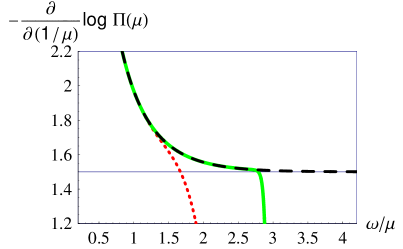
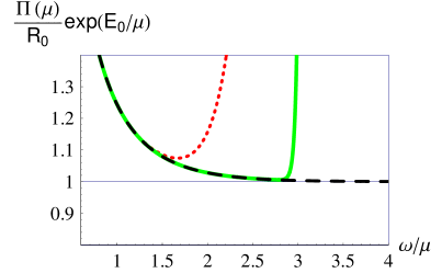
Fig. 2: Dashed (black) line – the calculation for the exact $\Pi(\mu)$; dotted (red) line – the calculation making use of the OPE for $\Pi(\mu)$ with 4 power corrections, solid (green) line – the same OPE with 100 power corrections.

In principle, it is possible to reach the plateau if one retains sufficiently many terms of the truncated OPE: the radius of convergence of the truncated OPE to the exact function $\Pi(\mu)$ increases with the increase of the number of terms taken into account, and, e.g., for $N>100$ the range of convergence already reaches the plateau (Fig. 2).

In practice, however, one can calculate only the first few terms and, consequently, the radius of convergence is rather small. For instance, with 4 terms the convergence region extends only up to values of $1/\mu$ for which the ground state gives 85% of the correlator.

The method of SVZ sum rules aims at extracting the parameters of the ground state from the first few terms of the OPE, e.g. in the region where the contribution of higher states is by far not negligible.

3 Sum rule

The sum rule claims the equality of the correlator calculated in the “quark” basis and in the hadron basis:

$$R_{0}\exp(-{E_{0}}/{\mu})+\int\limits_{z_{\rm cont}}^{\infty}dz\rho_{\rm phen}(z)\exp(-{z}/{\mu})=\int\limits_{0}^{\infty}dz\rho_{0}(z)\exp(-{z}/{\mu})+\mu^{3/2}\left[-\frac{\omega^{2}}{4\mu^{2}}+\frac{19}{480}\frac{\omega^{4}}{\mu^{4}}+\cdots\right],$$ (3.12)

with $\rho_{0}(z)=2\sqrt{z/\pi}$. Following nsvz , we use explicit expressions for the power corrections, but for the zero-order free-particle term we use its expression in terms of the spectral integral. The reason for this will become clear in a few lines.

Let us introduce the effective continuum threshold $z_{\rm eff}(\mu)$, different from the physical $\mu$-independent continuum threshold $z_{\rm cont}$, by the relation

$$\Pi_{\rm cont}(\mu)=\int\limits_{z_{\rm cont}}^{\infty}dz\,\rho_{\rm phen}(z)\,\exp(-z/\mu)=\int\limits_{z_{\rm eff}(\mu)}^{\infty}dz\,\rho_{0}(z)\,\exp(-z/\mu).$$ (3.13)

Generally speaking, the spectral densities $\rho_{\rm phen}(z)$ and $\rho_{0}(z)$ are different functions, so the two sides of (3.13) may be equal to each other only if the effective continuum threshold depends on $\mu$. In our model, we can calculate $\Pi_{\rm cont}$ precisely, as the difference between the known exact correlator and the known ground-state contribution, and therefore we can obtain the function $z_{\rm eff}(\mu)$ by solving (3.13). In the general case of a sum-rule analysis, the effective continuum threshold is not known and is one of the essential fitting parameters.

Making use of (3.13), we rewrite now the sum rule (3.12) in the form

$$R_{0}\exp({-{E_{0}}/\mu})=\Pi(\mu,z_{\rm eff}(\mu)),$$ (3.14)

where the cut correlator $\Pi(\mu,z_{\rm eff}(\mu))$ reads

$$\Pi(\mu,z_{\rm eff}(\mu))\equiv\frac{2}{\sqrt{\pi}}\int\limits_{0}^{z_{\rm eff}(\mu)}dz\sqrt{z}\exp(-z/\mu)+\mu^{3/2}\left[-\frac{\omega^{2}}{4\mu^{2}}+\frac{19}{480}\frac{\omega^{4}}{\mu^{4}}+\cdots\right].$$ (3.15)

As is obvious from (3.14), the cut correlator satisfies the equation

$$-\frac{d}{d(1/\mu)}\log\Pi(\mu,z_{\rm eff}(\mu))=E_{0}.$$ (3.16)

The cut correlator is the actual quantity which governs the extraction of the ground-state parameters.

The sum rule (3.14) allows us to restrict the structure of the effective continuum threshold $z_{\rm eff}(\mu)$. Let us expand both sides of (3.14) near $\omega/\mu=0$. The l.h.s. contains only even powers of $\sqrt{\omega/\mu}$; power corrections on the r.h.s. contain only odd powers of $\sqrt{\omega/\mu}$. In order that both sides match each other, the effective continuum threshold cannot be constant but should be a power series of the parameter $\sqrt{\omega/\mu}$:

$$z_{\rm eff}(\mu)=\omega\left[\bar{z}_{0}+\bar{z}_{1}\sqrt{\frac{\omega}{\mu}}+\bar{z}_{2}\frac{\omega}{\mu}+\cdots\right].$$ (3.17)

Inserting this series in (3.14) and expanding the integral on the r.h.s., we obtain an infinite chain of equations emerging at different orders of $\sqrt{\omega/\mu}$. These equations allow us to obtain for any $E_{0}$ and $R_{0}$ within a broad range of values a solution $z_{\rm eff}(\mu,R_{0},E_{0})$ which exactly solves the sum rule (3.12). Therefore, in a limited range of $\mu$ the OPE alone cannot say much about the ground-state parameters. What really matters is the continuum contribution, or, equivalently, $z_{\rm eff}(\mu)$. Without constraints on the effective continuum threshold the results obtained from the OPE are not restrictive!

The approximate extraction of $E_{0}$ and $R_{0}$ worked out in a limited range of values of $\mu$ becomes possible only by constraining $z_{\rm eff}(\mu)$. If these constraints are realistic and turn out to reproduce with a reasonable accuracy the exact $z_{\rm eff}(\mu)$, then the approximate procedure works well. If a good approximation is not found, the approximate procedure fails to reproduce the true value. Anyway, the accuracy of the extracted value is difficult to be kept under control. This conclusion is quite different from the results of QCD sum rules presented in the literature (see e.g. the review ck ). We shall demonstrate that a typical sum-rule analysis contains additional explicit or implicit assumptions and criteria for extracting the parameters of the ground state. Whereas these assumptions may lead to good central values of hadron parameters, the accuracy of the extracted values cannot be controlled within the method of QCD sum rules.

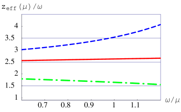
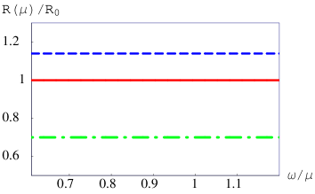
Fig. 3: Different choices of the effective continuum threshold $z_{\rm eff}(\mu)$ (a) and the corresponding $R(\mu)$ (b): 1 [solid (red) line] the exact effective continuum threshold as obtained by a numerical solution of (4.18) for $E=E_{0}$ and $R=R_{0}$. 2 [long-dashed (blue) line] the effective continuum threshold obtained by solving the sum rule (4.18) for $E=E_{0}$ and $R=0.7R_{0}$, 3 [dash-dotted (green) line] same as line 2, but for $E=E_{0}$ and $R=1.15R_{0}$.

4 Numerical analysis

In practice, one knows only the first few terms of the OPE, so one must stay in a region of $\mu$ bounded from below to guarantee that the truncated OPE series reproduces the exact correlator within a controlled accuracy. The “fiducial” svz range of $\mu$ is the range where, on the one hand, the OPE reproduces the exact expression better than some given accuracy (e.g., within 0.5%) and, on the other hand, the ground state is expected to give a sizable contribution to the correlator. If we include the first three power corrections, $\Pi_{1}$, $\Pi_{2}$, and $\Pi_{3}$, then the fiducial region lies at $\omega/\mu<1.2$ (see Fig. 3). Since we know the ground-state parameters, we fix $\omega/\mu>0.7$, where the ground state gives more than 60% of the full correlator. So our working range is $0.7<\omega/\mu<1.2$.

Obviously, if one knows the continuum contribution with a reasonable accuracy, one can extract the resonance parameters from the sum rule (3.12). We shall be interested, however, in the situation when the hadron continuum is not known, which is a typical situation in heavy-hadron physics and in studying properties of exotic hadrons. Can we still extract the ground-state parameters?

We shall seek the (approximate) solution to the equation

$$R\exp({-{E}/\mu})+\int\limits_{z_{\rm eff}(\mu)}^{\infty}dz\rho_{0}(z)\exp(-z/\mu)=\Pi_{\rm OPE}(\mu)$$ (4.18)

in the range $0.7<\omega/\mu<1.2$. Hereafter, we denote by $E$ and $R$ the values of the ground-state parameters as extracted from the sum rule (4.18). The notations $E_{0}$ and $R_{0}$ are reserved for the known exact values.

4.1 $\mu$-dependent effective continuum threshold.

In many interesting cases the ground-state energy can be determined, for instance, from experiment. However, fixing the ground-state energy $E$ equal to its known value $E_{0}$ does not help: for any $R$ within a broad range one can still find a solution $z_{\rm eff}(\mu,R)$ which solves the sum rule (4.18) exactly (Fig. 3). In order to extract $R$, one needs to constrain the effective continuum threshold; moreover, this constraint determines the actual value of $R$ which one obtains from the sum rule. If one requires, e.g., $z_{\rm eff}(\mu)>E_{0}$ for all $\mu$, then the sum rule (4.18) may be solved for any $R$ within the broad range $0.7<R/R_{0}<1.15$ (Fig. 3). Clearly, the sum rule alone, without knowing the continuum contribution, cannot determine $R$.

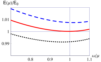
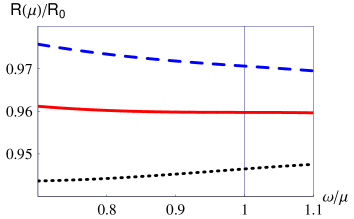
Fig. 4: Constant effective continuum threshold $z_{c}$: $E(\mu)$ for three different values of $z_{c}$ (a) and the corresponding $R(\mu)$ (b). Dotted (black) line - $z_{c}=2.4\,\omega$, solid (red) line - $z_{c}=2.454\,\omega$, dashed (blue) line - $z_{c}=2.5\,\omega$.

4.2 Constant effective continuum threshold.

Strictly speaking, a constant effective continuum threshold $z_{\rm eff}(\mu)=z_{c}={\rm const}$ is incompatible with the sum rule. Nevertheless, this Ansatz may work well, especially in our model: as can be seen from Fig. 3(a), the exact $z_{\rm eff}(\mu)$ is almost flat in the fiducial interval. Therefore, the HO model represents a very favorable situation for applying the QCD sum-rule machinery.

Now, one needs to impose a criterion for fixing $z_{c}$. A widely used procedure is the following jamin : one calculates

$$E(\mu,z_{c})\equiv-\frac{d}{d(1/\mu)}\log\Pi(\mu,z_{c}),$$ (4.19)

which now depends on $\mu$ due to approximating $z_{\rm eff}(\mu)$ by some constant. Then, one determines $\mu_{0}$ and $z_{c}$ as the solution to the system of equations

$$E(\mu_{0},z_{c})=E_{0},\qquad\left.\frac{\partial}{\partial\mu}E(\mu,z_{c})\right|_{\mu=\mu_{0}}=0,$$ (4.20)

yielding $z_{c}=2.454\,\omega$, $\mu_{0}/\omega=1$ (Fig. 4), and a good central-value estimate $R/R_{0}=0.96$, with $R$ being extremely stable in the fiducial range.

Note, however, a dangerous point: (i) a perfect description of $\Pi(\mu)$ with better than 1% accuracy, (ii) the deviation of $E(\mu,z_{c})$ from $E_{0}$ at the level of only 1%, and (iii) extreme stability of $R(\mu)$ in the full fiducial range leads to a 4% error in the extracted value of $R$! Clearly, this error could not be guessed on the basis of the other numbers obtained, and it would be wrong to estimate the error, e.g., from the range covered by $R$ when varying the Borel parameter $\mu$ within the fiducial interval.

5 Conclusions

Let us summarize the lessons we have learnt:

1. The knowledge of the correlator in a limited range of the Borel parameter $\mu$ is not sufficient for an extraction of the ground-state parameters with a controlled accuracy: Rather different models for the correlator in the form of a ground state plus an effective continuum lead to the same correlator.

2. The procedure of fixing the effective continuum threshold by requiring the average mass calculated with the cut correlator to reproduce the known ground-state mass jamin ; bz is not restrictive: a $\mu$-dependent effective continuum threshold $z_{\rm eff}(\mu)$, obtained as a solution of the sum rule (4.18), leads to the cut correlator (3.15) which automatically (i) reproduces exactly $E(\mu)=E_{0}$ for all values of the Borel parameter $\mu$, and (ii) yields a $\mu$-independent value of $R$ which, however, may be rather far from the true value.

3. Modeling the hadron continuum by a constant effective continuum threshold allows one to determine its value $z_{c}$ by, e.g., requiring the average energy $E(\mu)$ to be close to $E_{0}$ in the stability region. In the model under discussion (where the exact effective continuum threshold is, in fact, almost constant) one obtains in this way a good estimate $R/R_{0}=0.96$, with practically $\mu$-independent $R$. The unpleasant feature is that the deviation of $R$ from $R_{0}$ turns out to be much larger than the variations of $E(\mu)$ and $R$ over the fiducial range. Therefore, the systematic errors cannot be estimated by looking at the variation of $R$ within the fiducial domain of $\mu$.

Thus, we conclude that in those cases where the continuum contribution is not known (which is a typical situation encountered, e.g., in analyses of heavy-meson observables) the standard procedures adopted in a QCD sum-rule extraction of hadron parameters do not allow to control the systematic uncertainties. Consequently, no systematic errors for hadron parameters obtained with sum rules can be provided. Let us emphasize that the independence of the extracted values of hadron parameters from the Borel mass does not guarantee the extraction of their true values.

Nevertheless, in the model under consideration the sum rules give good estimates for the parameter $R_{0}$. This may be due to the following specific features of the model: (i) a large gap between the ground state and the first excitation that contributes to the sum rule; (ii) an almost constant exact effective continuum threshold in a wide range of $\mu$. Whether or not the same good accuracy may be achieved in QCD, where the features mentioned above are absent, is not obvious and requires more detailed investigations. One of the possible ways could be the application of different versions of sum rules to the same observable (see the discussion in lc_lms ; sr_lms ).

Presently, this shortcoming — the impossibility to control the systematic errors — remains the weak feature of the method of sum rules and an obstacle for using the results from QCD sum rules for precision physics, such as electroweak physics.

- (1) M. Shifman, A. Vainshtein, and V. Zakharov, Nucl. Phys. B147, 385 (1979).
- (2) V. Novikov, M. Shifman, A. Vainshtein, and V. Zakharov, Nucl. Phys. B237, 525 (1984).
- (3) A. I. Vainshtein, V. I. Zakharov, V. A. Novikov, and M. A. Shifman, Sov. J. Nucl. Phys. 32, 840 (1980).
- (4) V. A. Novikov et. al., Phys. Rep. 41, 1 (1978); M. B. Voloshin, Nucl. Phys. B154, 365 (1979); J. S. Bell and R. Bertlmann, Nucl. Phys. B177, 218 (1981); Nucl. Phys. B187, 285 (1981); V. A. Novikov, M. A. Shifman, A. I. Vainshtein, V. I. Zakharov, Nucl. Phys. B191, 301 (1981).
- (5) A. Le Yaouanc et. al., Phys. Rev. D62, 074007 (2000); Phys. Lett. B488, 153 (2000); Phys. Lett. B517, 135 (2001).
- (6) D. Melikhov and S. Simula, Phys. Rev. D62, 074012 (2000).
- (7) P. Colangelo and A. Khodjamirian, QCD sum rules: a modern perspective, hep-ph/0010175.
- (8) M. Jamin and B. Lange, Phys. Rev. D65, 056005 (2002).
- (9) P. Ball and R. Zwicky, Phys. Rev. D71, 014015 (2005).
- (10) W. Lucha, D. Melikhov, and S. Simula, Phys. Rev. D75, 096002 (2007); W. Lucha and D. Melikhov, Phys. Rev. D73, 054009 (2006); W. Lucha and D. Melikhov, Phys. Atom. Nucl. 70, 891 (2007).
- (11) W. Lucha, D. Melikhov, and S. Simula, Phys. Rev. D76, 036002 (2007); arXiv: 0707.4123 [hep-ph].
- (12) D. Melikhov, Phys. Rev. D53, 2460 (1996); Phys. Rev. D56, 7089 (1997); Eur. Phys. J. direct C4, 2 (2002) [hep-ph/0110087]; D. Melikhov and S. Simula, Eur. Phys. J. C37, 437 (2004).
- (13) D. Melikhov and B. Stech, Phys. Rev. D62, 014006 (2000).