Fermions in reduced dimensions (anyons, composite fermions, Luttinger liquid, etc.) Quantum wires (Electronic transport in nanoscale materials and structures) Theories and models of many-electron systems

Transport of interacting electrons through a potential barrier:
nonperturbative RG approach

Abstract

We calculate the linear response conductance of electrons in a Luttinger liquid with arbitrary interaction $g_{2}$, and subject to a potential barrier of arbitrary strength, as a function of temperature. We first map the Hamiltonian in the basis of scattering states into an effective low energy Hamiltonian in current algebra form. Analyzing the perturbation theory in the fermionic representation the diagrams contributing to the renormalization group (RG) $\beta$-function are identified. A universal part of the $\beta$-function is given by a ladder series and summed to all orders in $g_{2}$. First non-universal corrections beyond the ladder series are discussed. The RG-equation for the temperature dependent conductance is solved analytically. Our result agrees with known limiting cases.

Electron transport in nanowires has been studied theoretically for more than 20 years. Initially it was found that electron-electron interaction affects even the conductance of a clean wire [1, 2] . In the case of realistic boundary conditions, namely attaching ideal leads to the interacting quantum wire, the two-point conductance of a clean wire is that of the leads, equal to one conductance quantum per channel, irrespective of the (forward scattering) interaction [3, 4]. Alternatively, it has been argued that the screening of the external field by the interacting electron system leads to a renormalization of the conductance to its ideal value of unity [5]. The work of Kane and Fisher [2] and Furusaki and Nagaosa [6] showed, that interaction has a dramatic effect on the conductance in the presence of a potential barrier. For repulsive interaction these authors found that the conductance tends to zero as the temperature, $T$, or more generally, the excitation energy of the electrons approaches zero. This was shown at low temperature in the limits of weak potential barrier and strong potential barrier (tunneling limit), and at special values of the interaction parameter, $K=\frac{1}{2}$ and $K=\frac{1}{3}$, for all temperatures [2, 7, 8]. It has been argued, that these results apply to a contact free four-point measurement, which is best realized by measuring the absorption losses of an a.c. field in the limit $\omega\rightarrow 0$ [3, 4] (for a different view, see [5]).

We recall that the reason for the strong suppression of the conductance by a repulsive interaction is that the Friedel oscillations of the charge density around the potential barrier act as a spatially increasingly extended effective potential as the temperature is lowered. A proper treatment of the two-point conductance in the limit of weak interaction, taking into account the gradual build-up of the Friedel oscillations as the infrared cutoff is lowered has been given by Yue, Matveev and Glazman [9]. These authors used the perturbative RG for fermions to derive the conductance for an arbitrary (but short) potential barrier. A generalization of that approach to the case of two barriers has been given in [10].

In this letter we propose to extend the approach of Yue et al. to arbitrary strength of interaction. We argue that the $\beta$-function of the RG-equation for the conductance can be obtained in very good approximation by summing a class of contributions in all orders of the interaction. As we show below, this is possible in this case, at least at low temperature, since the class of diagrams with the maximum number of loops in any order, which are the ones contributing to the $\beta$-function, form a ladder series. At intermediate temperatures additional diagrams contribute small corrections to the $\beta$-function. The result of the solution of the RG-equation for the conductance, using the approximate $\beta$-function thus obtained, is found to agree with all known results on the scaling behavior of the conductance, including the case $K=\frac{1}{2}$, but goes far beyond: it is valid for any interaction strength $K$ and any potential scattering strength. A careful analysis of the dependence of the result on the cutoff procedure chosen shows that certain terms in the $\beta$-function are not universal and depend on the cutoff scheme.

The Model. We consider a one-dimensional system (coordinate $x$) of spinless electrons subject to a potential barrier at $x=0$. The barrier is characterized by transmission and reflection amplitudes $t=\tilde{t}=\cos\theta$, $r=-\tilde{r}^{\ast}=i\sin\theta e^{i\phi}$ with negligible energy dependence in the energy range of interest (width of order of temperature, $T$, around the Fermi energy, $\epsilon_{F}$). We assume the extension of the barrier, $a$, to be narrow, $ak_{F}\ll 1$, and neglect all interaction processes both close to the barrier $|x|<a$ (here $k_{F}$ is the Fermi wave number) and in the leads, $|x|>L$. Beyond the large scale $L$ the system is assumed non-interacting, which allows for an asymptotic single-particle scattering states representation.

If $c_{1k}^{+}$ and $c_{2k}^{+}$ are operators creating electrons in right-moving and left-moving single particle scattering states of the barrier ($k>0$), we may define the electron creation operator $\psi^{+}(x)$ as

$$\psi^{+}(x) = \left\{\Theta(-x)\left[\psi_{1}^{+}(x)+r\psi_{1}^{+}(-x)+\tilde{t}\psi_{2}^{+}(x)\right]\right.$$ (1)

$$+\left.\Theta(x)\left[t\psi_{1}^{+}(x)+\tilde{r}\psi_{2}^{+}(-x)+\psi_{2}^{+}(x)\right]\right\}\,,$$

where $\psi_{1,2}^{+}(x)=\int_{0}^{\infty}\frac{\upd k}{2\pi}e^{\pm ikx}c_{1,2k}^{+}$.

It is convenient to define current operators $J_{\mu}(x)$, $\mu=0,1,2,3$ by $J_{\mu}(x)=\frac{1}{2}\Sigma_{\alpha,\beta=1,2}\psi_{\alpha}^{+}(\alpha x)\tau_{\alpha\beta}^{\mu}\psi_{\beta}(\beta x)$, where $\tau^{\mu}$ are the Pauli matrices plus the unit matrix, $\psi_{\alpha}^{+}(\alpha x)=\psi_{1}^{+}(x)$ or $\psi_{2}^{+}(-x)$ for $\alpha=1,2$. We call $J_{0}$ the isocharge current and the vector $\vec{J}=(J_{1},J_{2},J_{3})$ the isospin current; these operators obey $U(1)$ and $SU(2)$ Kac-Moody algebras, respectively [11, 12]. In this paper we will not make use of these relations, but instead will work in the fermion representation. Nonetheless, the representation allows one to work in the chiral fermion representation.

The particle density operators for incoming $(i)$ and outgoing $(o)$ particles in terms of the $J_{\mu}$’s are given by (here $x>0$ )

$$\rho_{iR,L}(\mp x) = \psi_{1,2}^{+}(\mp x)\psi_{1,2}(\mp x)=J_{0}(-x)\pm J_{3}(-x)\,,$$

$$\rho_{oR}(x) = \left[t\psi_{1}^{+}(x)+\tilde{r}\psi_{2}^{+}(-x)\right]\left[t^{\ast}\psi_{1}(x)+\tilde{r}^{\ast}\psi_{2}(-x)\right]$$

$$= J_{0}(x)+\tilde{J}_{3}(x)$$

$$\rho_{oL}(-x) = \left[r\psi_{1}^{+}(x)+\tilde{t}\psi_{2}(-x)\right]\left[r^{\ast}\psi_{1}(x)+\tilde{t}^{\ast}\psi_{2}(-x)\right]$$ (2)

$$= J_{0}(x)-\tilde{J}_{3}(x)\,.$$

Here $\tilde{J}_{3}=(R\vec{J})_{3}$ is the third component of the isospin current vector $\vec{J}$ rotated by the orthogonal matrix $R_{\mu\nu}$ with $R_{33}=|t|^{2}-|r|^{2}=\cos 2\theta$, $R_{32}=\mbox{Im}\{t\widetilde{r}^{\ast}+\widetilde{t}r^{\ast}\}=-\sin 2\theta\cos\phi$, $R_{31}=\mbox{Re}\{t\widetilde{r}^{\ast}-\widetilde{t}r^{\ast}\}=\sin 2\theta\sin\phi$.

We consider a model with interaction constant $g_{2}$ (no backscattering, no Umklapp processes). The Hamiltonian is given by $H=H_{0}+H_{1}$, with

$$H_{0} = 2\pi v_{F}\int_{0}^{\infty}\upd x\left[J_{0}^{2}(-x)+J_{0}^{2}(x)+J_{3}^{2}(-x)+\tilde{J}_{3}^{2}(x)\right]\,,$$

$$H_{1} = 2g_{2}\int_{a}^{L}\upd x\left[J_{0}(-x)J_{0}(x)-J_{3}(-x)\tilde{J}_{3}(x)\right]\,,$$ (3)

where $v_{F}$ is the Fermi velocity. The forward scattering interaction $g_{4}$ of like-movers may be absorbed into redefinition of $v_{F}$ in the usual way [11]. In Fig. 1 we show in a pictorial way our parametrization of the fermionic densities and the interaction, $H_{1}$. In Fig. 1a the $g_{2}$-interaction processes are shown in the usual scattering configuration. The representation in terms of the currents $J_{\mu}$ is in the chiral basis (all particles moving to the right, see Fig. 1b), which leads to a seemingly nonlocal interaction. It should be clear that electrons in the left half space ($x<0$) are not affected by the barrier yet, whereas electrons on the right ($x>0$) are. Note that in the case of perfect reflection, $t=0$, we have $\tilde{J}_{3}=-J_{3}$ and the observable densities (see below) form an Abelian $U(1)$ sub-algebra of $SU(2)$. This is the case of “open boundary bosonization”, which allows a complete and rather simple analysis. [13] One can also show that the $J_{3}$ part of Eq. (3) can be reduced by a canonical transformation $H^{\prime}=U^{\dagger}HU$ to the Hamiltonian with the interaction part

$$H_{1}^{\prime}=v_{F}\mathbf{B}.\mathbf{J}(x=0)-2g_{2}\int_{a}^{L}\upd x\,J_{3}(-x)J_{3}(x)\,,$$ (4)

here $U=\exp i\int_{0}^{\infty}\upd x\mathbf{B}.\mathbf{J}(x)$ and $\mathbf{B}=2\theta(\cos\phi,\sin\phi,0)$. [14] The first term in (4) corresponds to the rotation of the incoming isospin current $\mathbf{J}$ by the “magnetic field”, $\mathbf{B}$, at the origin, Fig. 1b. Eq. (4) thus resembles the Hamiltonian for the Kondo problem in the current algebra approach. [12] The major simplification in our case is the classical nature of $\mathbf{B}$, as opposed to the quantum Kondo spin $\mathbf{S}$, see [12].

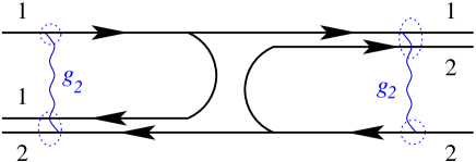
(a) (b)

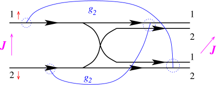
Figure 1: (a)The interaction of the left- and right-going densities in the basis of scattered waves. (b) The interaction of the left- and right-going densities in the chiral basis, corresponding to non-local interaction, Eq. (3).

Current and conductance. The total electron density $\rho(x)$ is given by

$$\rho(x) = \left[\rho_{iR}(x)+\rho_{oL}(x)\right]{\Theta}(-x)+\left[\rho_{oR}(x)+\rho_{iL}(x)\right]{\Theta}(x),$$ (5)

$$= J_{0}(-x)+J_{0}(x)+\mbox{sgn}(x)\left[-J_{3}(-|x|)+\tilde{J}_{3}(|x|)\right]\,,$$

$$= \rho_{c}(x)+\rho_{s}(x)\,,$$

where subscript $c(s)$ refers to isocharge (isospin) components. From the continuity equation $\partial_{t}\rho(x)=-\partial_{x}j(x)=-i[\rho(x),H]$ one finds the current

$$j(x) = v_{F}\left[J_{0}(x)-J_{0}(-x)+J_{3}(-|x|)+\tilde{J}_{3}(|x|)\right]$$ (6)

$$= j_{c}(x)+j_{s}(x)\,.$$

We now consider the linear response to an applied voltage $V(x,t)=\frac{1}{2}V(t)\mbox{sgn}(x)$, which is seen to couple only to the isospin components, $\rho_{s}$, of the density operator. The conductance is then given by (in units of $e^{2}/2\pi\hbar$)

$$G(x,t)=-2\pi i\Theta(t)\;\left\langle\left[j_{s}(x,t)\;,\;\int_{0}^{\infty}\upd y\;\rho_{s}(y,0)\right]\right\rangle\,,$$ (7)

where we used the fact that correlation functions mixing the isocharge and isospin sectors vanish.

Perturbation theory in $g_{2}$. The contributions to $G(\Omega_{m})$ in n-th order of $g_{2}$ may be calculated with the help of Feynman diagrams in the position-energy representation ($\Omega_{m}$ is the external Matsubara frequency). We draw $n$ vertical wavy lines in parallel, the upper endpoint of the $i$-th line at $-x_{i}$ with isospin matrix $\frac{1}{2}\tau_{\alpha\beta}^{3}$ , the lower one at $x_{i}$ with matrix $\frac{1}{2}R_{3\mu}{\tau}_{\alpha\beta}^{\mu}$ attached and carrying the factor $-2g_{2}$ ; $\alpha,(\beta)$ are isospin indices of ingoing, (outgoing) fermion lines. The external vertices are at $-x$ with matrix $\frac{1}{2}\tau_{3}$ and at $y$ with matrix $\frac{1}{2}(R\vec{\tau})_{3}$. The vertex points are connected by Green’s functions

$$\mathcal{G}(x\;;\;\omega_{n})=-\frac{i}{v_{F}}\mbox{sign}(\omega_{n})\Theta(\omega_{n}x)e^{-\omega_{n}x/v_{F}}\,,$$ (8)

where the $\omega_{n}$ are Matsubara fequencies $\omega_{n}=(2n+1)\pi T$. All internal $x$ -variables are integrated on the positive semi axis. The trace over the product of all isospin matrices in each fermion loop is taken and a factor of $1/n!$ is applied to each n-th order diagram. The limit $\Omega_{m}\rightarrow+0$ is taken at the end.

The incoming component of $\rho_{s}(y),J_{3}(-y)$, only contributes in zeroth order: $G_{i}^{(0)}=\frac{1}{2}$. Adding the contribution from the outgoing component one finds

$$G^{(0)}=\frac{1}{2}(1+\cos 2\theta)=\cos^{2}\theta=\left|t\right|^{2}\,.$$ (9)

The diagrams of first order in $g_{2}$ are shown in Fig. 2. Note that the “vertex correction type” diagram, Fig. 2c, is $\propto\Omega$ and will be dropped. One finds

$$G^{(1)}=-\frac{g_{2}}{4\pi}\sin^{2}(2\theta)\;\ln\frac{T_{0}}{T}\,,$$ (10)

in agreement with [9]. The ultraviolet cutoff, $T_{0}$, is determined by the width of the potential barrier $a$ as $T_{0}=v_{F}/(2\pi a)$, the infrared cutoff arises at finite $T>v_{F}/L$ through the Green’s function at time $t=0$: $\mathcal{G}(2a\;;\;t=0)\sim T/\sinh(2\pi Ta/v_{F})$. In the limit of zero temperature the finite-$T$ logarithm $\Lambda\equiv\ln({T_{0}}/{T})$ is replaced by the zero temperature expression $\Lambda_{0}\equiv\ln(L/a)$.

Figure 2: Three Feynman diagrams, depicting the first order in $g_{2}$ contribution to the conductance. The other three diagrams are obtained from these by reversing the direction of fermionic propagation.

In $n$-th order the diagrams with only one loop contribute the scale dependent terms $[\ln T_{0}/T]^{n}$. Our prinicipal observation here is that the diagrams with the maximum number of loops ($n$ loops) contribute linearly in logarithm $\propto\ln(T_{0}/T)$. They form a set of ladder diagrams. The diagrams linear in $\ln(T_{0}/T)$ but not contained in this ladder series will be discussed  below. The sum of all ladder diagrams (see Fig. 3) may be calculated, and will be denoted by $\bar{L}(x_{1},x_{2};\omega_{n})$. Later we will need the integrated quantity $L(x_{1};\omega_{n})=\int_{0}^{\infty}\upd x_{2}e^{-\omega_{n}x_{2}}\quad\bar{L}(x_{1},x_{2};\omega_{n})$, which obeys the integral equation

$$L(x;\omega) = -ge^{-\omega x}\left[4\pi+\omega(Y+\frac{g}{2})\int_{0}^{\infty}\upd ze^{-\omega z}L(z;\omega)\right]$$ (11)

$$+ \frac{1}{2}g^{2}\omega\int_{0}^{\infty}\upd z\;\;e^{-\omega|x-z|}L(z;\omega)\,.$$

Figure 3: Ladder series, $\bar{L}(x_{1},x_{2};\omega_{n})$, describing the combined effect of interaction and barrier, and leading to a linear-in-logarithm $\ln(T_{0}/T)$ contribution to conductance.

Here we defined $Y=\cos 2\theta$, $g=g_{2}/2\pi$ and we use units with $v_{F}=1$. The Eq. (11) is of Wiener-Hopf type and its solution is $L(x;\omega_{n})=-4\pi gbe^{-\omega_{n}px}$ where $p=\sqrt{1-g^{2}}$ and $b=(1+p)/(1+p+gY)$. The conductance contribution $G^{(L)}$ in linear order in $\ln\frac{T_{0}}{T}$, summed to all orders in $g_{2}$, is given by

$$G^{(L)} = \frac{1-Y^{2}}{4}T^{2}\sum_{\epsilon,\omega}\int_{0}^{\infty}\upd x_{1}\upd x_{2}\upd y\bar{L}(x_{1},x_{2};\omega)\mathcal{G}(x_{1}-x;\epsilon)$$ (12)

$$\times \mathcal{G}(-x_{1}-x_{2};\epsilon-\omega)\mathcal{G}(x_{2}-y;\epsilon)\mathcal{G}(y+x;\epsilon+\Omega)\,.$$

Taking the limit $\Omega\rightarrow 0$ at $x\gg v_{F}/T$ one finds

$$G^{(L)}=\frac{-g(1-Y^{2})}{1+\sqrt{1-g^{2}}+gY}\;\ln\frac{T_{0}}{T}\equiv-\widetilde{g}(1-Y^{2})\ln\frac{T_{0}}{T}\,.$$ (13)

Comparing eq.(13) with eq.(10) we see that the resummation corresponds to dressing of the interaction, $g\to\widetilde{g}$.

Renormalization group approach. In perturbation theory the $n$-th order contribution in $g_{2}$ is a polynomial in $\Lambda$ of degree $n$. If the theory is renormalizable, all terms with higher powers of $\Lambda$ should be generated by a renormalization group equation for the scaled conductance, $G(\Lambda)$, or equivalently for $Y(\Lambda)=2G(\Lambda)-1$. Our approximation to the $\beta$-function of the RG equation is given by the prefactor of $\ln\frac{T_{0}}{T}$ in the perturbation theory result (13), with $Y$ replaced by $Y(\Lambda)$:

$$\frac{dY}{d\Lambda}=-\frac{2g(1-Y^{2})}{1+\sqrt{1-g^{2}}+gY}=\beta_{L}(Y)\,.$$ (14)

Introducing the Luttinger parameter, $K=[(1-g)/(1+g)]^{1/2}$, we can rewrite (14) as

$$\frac{d\Lambda}{dY}=-\frac{1}{2(Y+1)(K^{-1}-1)}-\frac{1}{2(1-Y)(1-K)}\,,$$ (15)

which is easily integrated (see below). We note that (15) has a kind of duality symmetry: it is invariant under $K\rightarrow K^{-1}$, $Y\rightarrow-Y$. For weak interaction, we expand $K^{\pm 1}\simeq 1\mp g$ and recover the result by [9]. In the limiting cases of nearly transparent and nearly perfectly reflecting barrier, we recover the results by [2, 6], with $G\sim\left({T}/{T_{0}}\right)^{2(\frac{1}{K}-1)}$ and $1-G\sim\left({T_{0}}/{T}\right)^{2(1-K)}$, respectively.

A remaining question concerns the existence of additional terms in the RG $\beta$-function, not contained in the ladder series (15) (cf. [15]). To answer it, we have calculated $G$ using computer algebra up to fourth order ($\sim 40,000$ diagrams). [14] The results are summarized as follows. In higher orders we find both leading ($\sim g^{n}\Lambda^{n}$) and subleading ($\sim g^{n}\Lambda^{k}$, $k<n$) contributions. Most of these terms correspond to Eq. (14). However, starting from third order of $g$ we find also subleading contributions linear in $\Lambda$, which are explicitly different from the form (15) and arise from diagrams depicted in Fig. 4. Adding these terms to the $\beta$-function of (14) we obtain

$$\frac{dY}{d\Lambda}=-\widetilde{g}(1-Y^{2})+g^{3}(1-Y^{2})^{2}(c_{3}-gYc_{4}+O(g^{2}))\,,$$ (16)

with $\widetilde{g}$ the above result of the ladder resummation, $c_{3}=\pi^{2}/12$ and $c_{4}=0.238\ldots$. Notice the different power of $(1-Y^{2})$ in front of the extra terms in (16), which renders these terms irrelevant in the limits $G\rightarrow 0$, $G\rightarrow 1$.

Figure 4: Skeleton Feynman graphs, leading to lowest order logarithmic contribution, $g^{3}\Lambda$, beyond ladder series.

Before proceeding further we should discuss the issue of universality of the logarithmic corrections, i.e. their dependence on the cutoff regularization scheme. Interpreting the ladder summation as a dressing of the interaction, Fig. 3, $g\rightarrow\widetilde{g}$, the ladder result (14) thus corresponds to only one non-trivial Matsubara frequency summation, which amounts to a ”one-loop” RG correction in the usual classification. In this case the scale invariant linear logarithmic contribution is not sensitive to the cutoff regularization, i.e. when $L$ exceeds the inverse temperature $\ln L/a\rightarrow\ln(v_{F}/2\pi Ta)$ and the prefactor of the logarithm is preserved. In other words, these contributions are universal in the RG sense. In the order $g^{2}$, non-trivial ”two-loop” corrections to (14) are absent. In the order $g^{3}$ the ”three-loop” contributions are divided into two groups. The first group consists of the first diagram in Fig. 4 and its symmetry-related partners: its contribution to $G$ is $\frac{\pi^{2}}{24}\Lambda g^{3}(1-Y^{2})^{2}$ ; this linear-in-$\Lambda$ correction is again universal. The additional diagrams in Fig. 4 contain both $\Lambda^{3}$ and $\Lambda$ contributions. In this situation the linear-in-$\Lambda$ terms contributing to the $\beta-$function are dependent on the cutoff scheme, i.e. are non-universal. The above cited value $c_{3}=\pi^{2}/12$ corresponds to $T=0$ , i.e. the hard infrared cutoff $L$ in real space. If we calculate corrections at $T\gg v_{F}L^{-1}$, then we obtain the soft cutoff result $c_{3}=1/4$ instead, in agreement with [16] ; we use this latter value below.

Inverting (16) we get ${d\Lambda}/{dY}=(\beta_{L}(Y))^{-1}-g\;h(g,Y)$ where $h(g,Y)=c_{3}-gYO(1)+\ldots$ for small $g$ has been defined. Notice that in the non-ladder corrections $g\;h(g,Y)$ we may substitute $g$ by its renormalized value $g\rightarrow\widetilde{g}$. Truncating at lowest level beyond the ladder series, we get

$${d\Lambda}/{dY}\simeq\left[{\beta_{L}(Y)}\right]^{-1}-c_{3}\widetilde{g}\;\,.$$ (17)

Integrating the latter equation we have

$$\left({T}/{T_{0}}\right)^{2(1-K)} = {\Phi(G)}/{\Phi(G_{0})}\,,$$ (18)

$$\Phi(G) = \frac{G^{K}}{1-G}\left(K+G(1-K)\right)^{4c_{3}(1-K)}\,,$$

with $c_{3}=1/4$ and the assumed initial condition $G=G_{0}$ at $T=T_{0}$.

The equation (18) is the central result of this paper. Let us discuss it in more detail. The above ladder approximation(14) would correspond to setting $c_{3}=0$ in (18). It is seen that the above cited scaling-law dependences of $G$ on $T$ remain asymptotically exact at $G\rightarrow 0$ and $G\rightarrow 1$. The existence of terms in the $\beta$-function beyond the ladder series modifies the behavior of the conductance at intermediate values $G\sim 1/2$, and the role of $h(g,Y)\sim 1/4$ can hence be largely viewed as a redefinition of the cutoff energy $\ln T_{0}\rightarrow\ln T_{0}+O(gG_{0})$, when going from higher to lower $T$. The duality symmetry, Eq. (15), between the scaling exponents is preserved, $T^{2(K-1)}\to T^{2(K^{-1}-1)}$, in contrast to the recent claim in [17] ; the breaking of duality reported in [17] might be connected to the approximate character of the solution for the set of flow equations there.

Let us also compare our findings to exact expressions available from the thermodynamic Bethe Ansatz method. In the particular case of $K={1}/{2}$ ($g=3/5$) the conductance $G$ is obtained as a closed analytic function of $T$. [2, 7] Our Eq. (18) reduces to a quadratic equation, with relevant solution

$$G=\frac{4\tau^{2}}{1+4\tau^{2}+\sqrt{1+16\tau^{2}}}\,,\quad\tau=\frac{T}{T_{0}}\frac{\left|t\right|\sqrt{1-\frac{1}{2}|r|^{2}}}{\left|r\right|^{2}}\,,$$ (19)

where $\left|t\right|$, $\left|r\right|$ are the bare transmission and reflection amplitudes.

At high temperatures the result reported in [2, 7] tends to the clean limit value for a four-point measurement, $G=\frac{1}{2}$; here we assume that the two-point conductance is obtained by multiplying the latter result by a factor of $1/K$ equal to $2$ in order to make contact with our theory. Fixing the overall scale $T^{\ast}$ in both solutions ($\tau\equiv{T}/{T^{\ast}}$) by their high-temperature behavior, $G\simeq 1-\tau^{-1}$, we show the overall picture in Fig. 5. It is seen that the result of the ladder summation overestimates the renormalization of the barrier, predicting smaller conductance at low $T$. At the same time the adjustment of the ladder summation by $c_{3}=1/4$, Eqs.(17), (18), (19), gives excellent agreement with the exact solution [2, 7], with a relative deviation not exceeding 4 % in the whole temperature range.

In case $K={1}/{3}$ ($g=4/5$), relevant for the description of point conductance between the quantum Hall edge states, [8] we do not have a closed analytic expression for $G(T)$. It is however possible to make a comparison to our theory. We fix the overall temperature scale by adopting $G\simeq 1-\tau^{-4/3}$ at high temperatures, then we have $G\simeq 9\tau^{4}$ from our Eq. (18). Multiplying again the result reported in [8] by a factor of $1/K=3$, we have $G\simeq 10.0638\tau^{4}$ at low $T$, whose prefactor is within 12 % from our value. We may thus conclude that our result (18) provides a very good approximation even in the strongly interacting case $g\sim 1$, i.e. it is sufficient for all practical purposes.

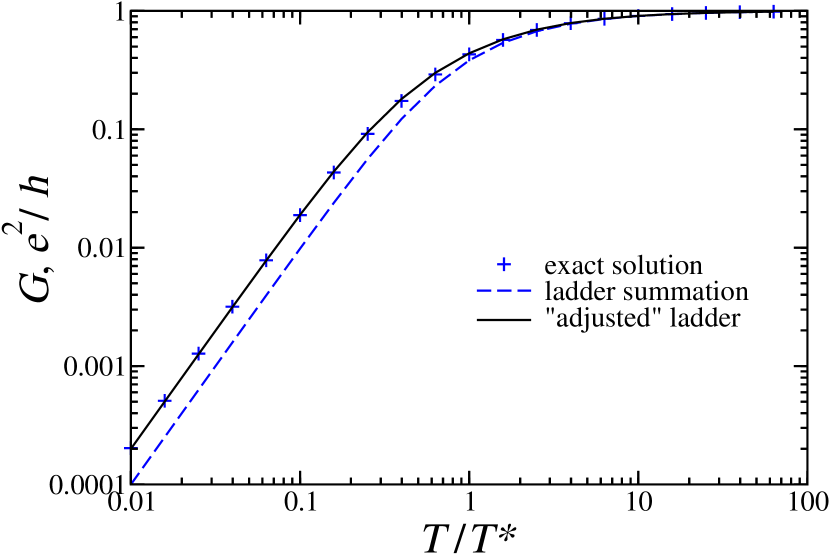
Figure 5: Conductance as a function of temperature for $K=1/2$. The exact result available from TBA (multiplied by factor 2) is shown by pluses. [2, 7] The results of ladder summation, (18) with $c_{3}=0$, are shown by dashed line ; the result of Eq. (18) with the adjusting term $c_{3}=1/4$ is shown by solid line.

Conclusion. In this letter we presented a theory of transport of interacting electrons through a potential barrier, in the linear response regime and at all temperatures, for any short range barrier and for any forward scattering interaction. We employed a representation in terms of chiral fermions, which greatly simplifies the perturbation theory in the interaction parameter $g_{2}$. In this way the scale dependent contributions to the conductance may be studied systematically. At low energies long range correlations lead to logarithmically diverging terms in the form of powers of $\Lambda=\ln\frac{T_{0}}{T}$.

In particular, the terms linear in $\Lambda$ may be summed to all orders in $g_{2}$, and the prefactor may be identified with the $\beta$-function of the renormalization group equation for the conductance as a function of the scaling variable $\Lambda$. At intermediate temperatures additional small corrections to the $\beta$-function were found in third and higher orders of perturbation theory. Approximating these additional terms by the lowest order (in $g_{2}$ ) gave excellent agreement with the known exact result at $K=\frac{1}{2}$. This appears to be one of the few cases where the $\beta$-function can be determined beyond perturbation theory. Our results are in agreement with all known results, where applicable, but go far beyond. The RG-equation may be integrated analytically to give the conductance as an implicit function of the temperature. The method we describe here is quite general and may be of value for calculating transport properties of the model out of equilibrium or of other models in which the $\beta$-function may be obtained by summing a ladder series.

- [1] \NameApel W. Rice T. M. \REVIEWPhys. Rev. B26 1982 7063.
- [2] \NameKane C. L. Fisher M. P. A. \REVIEWPhys. Rev. Lett.68 1992 1220 ; \REVIEWPhys. Rev. B46 1992 15233.
- [3] \NameMaslov D. L. Stone M. \REVIEWPhys. Rev. B52 1995 R5539.
- [4] \NameSafi I. Schulz H. J. \REVIEWPhys. Rev. B52 1995 R17040.
- [5] \NameOreg Y. Finkel’stein A. M. \REVIEWPhys. Rev. B54 1996 14265
- [6] \NameFurusaki A. Nagaosa N. \REVIEWPhys. Rev. B47 1993 4631.
- [7] \NameWeiss U., Egger R. Sassetti M. \REVIEWPhys. Rev. B52 1995 16707.
- [8] \Name Fendley P., Ludwig A. W. W. Saleur H. \REVIEWPhys. Rev. Lett.7419953005; \REVIEWPhys. Rev. B521995 8934.
- [9] \NameYue D., Glazman L. I. Matveev K. A. \REVIEWPhys. Rev. B49 1994 1966.
- [10] \NamePolyakov D. G. Gornyi I. V. \REVIEWPhys. Rev. B 68 2003 035421.
- [11] \NameGogolin A. O., Nersesyan A. A. Tsvelik A. M. \BookBosonization and Strongly Correlated Systems \PublCambridge University Press, Cambridge \Year1998.
- [12] \Name Affleck I. \REVIEW Nucl. Phys. B336 1990 517 ; \Name Affleck I. Ludwig A. W. W. \REVIEW Nucl. Phys. B360 1991 641.
- [13] \Name Fabrizio M. Gogolin A.O. \REVIEWPhys. Rev. B51 1995 17827.
- [14] \Name Aristov D. N. Wölfle P. to be published.
- [15] \Name Ludwig A. W. W. Wiese K. J. \REVIEW Nucl. Phys. B 661 2003 577.
- [16] \Name Lukyanov S. L. Werner Ph. \REVIEWJ. Stat. Mech. 2007 P06002; \NameLukyanov S. L. private communication.
- [17] \NameEnss T., Meden V., Andergassen S., Barnabé-Thériault X., Metzner W., Schönhammer K. \REVIEWPhys. Rev. B71 2005 155401.