A non-linear dynamical systems approach to source compression for constrained sources

Abstract

We have recently established a strong connection between the Tent map (also known as Generalized Luroth Series or GLS which is a chaotic, ergodic and lebesgue measure preserving non-linear dynamical system) and Arithmetic coding which is a popular source compression algorithm used in international compression standards such as JPEG2000 and H.264. This was for independent and identically distributed binary sources. In this paper, we address the problem of compression of ergodic Markov binary sources with certain words forbidden from the message space. We shall show that GLS can be modified suitably to achieve Shannon’s entropy rate for these sources.

1 Introduction

Emerging trends in data acquisition and imaging technologies have resulted in a rapid increase in the volume of data. Hence source coding (or data compression) continues to occupy an important area of research in the design of communication and storage systems. Shannon, the father of information theory, provided the definition of Entropy as the ultimate limit of lossless data compression. Ever since, there have been a number of compression algorithms which tries to achieve this limit.

The source coding problem is stated as follows: Given an independent and identically distributed (i.i.d) binary source $X$ emitting bits of information in the absence of noise, how do we obtain the shortest lossless representation of this information? Source coding is also known as entropy coding or data compression and is an important part of most communication systems [1].

Shannon in his 1948 masterpiece [2] defined the most important concept of Information Theory, namely ‘Entropy’. Shannon’s Entropy of a source $H(X)$ is defined as the amount of information content or the amount of uncertainty associated with the source, or equivalently the least number of bits required to represent the information content of a source without any loss. Shannon proposed a method (Shannon-Fano coding [3]) that achieves this limit as the block-length (number of symbols taken together) for coding increases asymptotically to infinity. Huffman [4] proposed what are called minimum-redundancy codes with integer code-word lengths that achieve Shannon’s Entropy in the limit of the block-length tending to infinity. However, there are problems associated with both Shannon-Fano coding and Huffman coding (and other similar techniques). As the block-length increases, the number of alphabets exponentially increase, thereby increasing the memory needed for storing and handling. Also, the complexity of the encoding algorithm increases since these methods build code-words for all possible messages for a given length instead of designing the codes for a particular message at hand. Another disadvantage of all such methods is that they do not lend themselves easily to an adaptive coding technique [1]. The idea of adaptive coding is to update the probability model of the source during the coding process. Unfortunately, for both Huffman and Shannon-Fano coding, the updating of the probability model would result in re-computation of the code-words for all the symbols which is an expensive process.

Recently, we have proposed a new approach to address the source coding problem using a dynamical systems perspective [5]. We modeled the information bits of the source $X$ as measurements of a non-linear dynamical system. Since measurement is rarely accurate, we treat these measured bits of information as a symbolic sequence [6] of the Tent map [7] and their skewed cousins. Source coding is seen as determination of the initial condition that has generated the given symbolic sequence. Subsequently, we established that such an approach leads us to a well known entropy coding technique (Arithmetic Coding) which is optimal for compression. Furthermore, this new approach enabled a robust framework for joint source coding and encryption.

In this paper, we focus on constrained sources where certain words are forbidden from its message space. Such sources are longer i.i.d because they violate the independence assumption (most natural sources are not independent, for e.g., english text is clearly not independent). We consider only ergodic Markov sources in this paper. We propose a non-linear dynamical systems approach to compress messages from these constrained sources.

2 Embedding an i.i.d source

We shall first start with an i.i.d source $X$ which can be thought of as emitting a sequence of random variables $\{X_{1},X_{2},\ldots,X_{N}\}$. Each random variable takes values independently from the common alphabet $\mathcal{A}=\{a_{1},a_{2},\ldots,a_{|\mathcal{A}|}\}$ with probabilities $\{p_{1},p_{2},\ldots,p_{|\mathcal{A}|}\}$ respectively. A message from this source is a particular sequence of values $M=\{x_{1},x_{2},\ldots,x_{N}\}$ where $x_{1}$ is drawn from $X_{1}$, $x_{2}$ from $X_{2}$ and so on. Since these are i.i.d, we can think of them as being drawn from the common random variable $X$ (we use the notation $X$ for both the source and the common random variable). We always deal with finite sized alphabets ($|\mathcal{A}|<\infty$) and finite length messages ($N<\infty$) since real-world messages are always finite in length.

Our aim is to embed this i.i.d source into a non-linear discrete dynamical system. The reason for doing this will be clear soon. To this end, we model the i.i.d source as a 0-order Markov source (memoryless source). Each alphabet can be seen as a Markov state. Since these are independent, the transition probability from state $i$ to state $j$ is equal to the probability of being in state $j$. In other words, $P_{ij}=P(X_{r+1}=j|X_{r}=i)=P(X_{r+1}=j)$.

We wish to embed this 0-order Markov source into a non-linear dynamical system $(\Omega,\Im,T,\mu)$ where $\Omega$ is the set $[0,1)$, $\Im$ is the Borel $\sigma$-algebra on $[0,1)$, $T$ is the measure preserving transformation (yet to be defined) and $\mu$ is the invariant measure. Here we consider the probability measure (or Lebesgue measure) as the invariant measure. We now need to define $T$ which preserves the Lebesgue measure and which can simulate the 0-order Markov source faithfully.

2.1 GLS embeds the i.i.d source

The non-linear discrete dynamical system known as Generalized Luröth series (GLS) [8] (Figure 1) embeds the 0-order Markov source. We list the important properties of GLS which enable this embedding:

1. The number of partitions (disjoint intervals which cover the space, also known as cylinders) of the GLS is equal to the size of the alphabet.

2. Each alphabet is used to ‘label’ a partition.

3. The size of each partition is equal to the probability of the corresponding alphabet.

4. The map is linear and surjective on each of the partitions.

5. GLS preserves the Lebesgue measure [8].

6. Successive digits (or symbols) of the GLS are i.i.d.

7. Every unique sequence of digits (or symbols) maps to a unique point $x$ in [0,1) under $T$. In other words, every point $x$ has an unique representation in terms of the alphabets of GLS. We call $x$ as the initial condition corresponding to the symbolic sequence (any sequence of digits composed from the alphabets associated with the partitions).

8. GLS is chaotic (positive Lyapunov exponent and positive Topological entorpy).

9. The GLS transformation $T$ on [0,1) is isomorphic to the Bernoulli shift [8]. Hence GLS is ergodic with Lebesgue as the invariant measure.

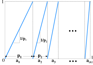
Figure 1: GLS embeds an i.i.d source faithfully. The digits $\{a_{1},a_{2},\ldots,a_{|\mathcal{A}|}\}$ are the alphabets from $\mathcal{A}$. The lengths of the intervals are precisely the respective probabilities $\{p_{1},p_{2},\ldots,p_{|\mathcal{A}|}\}$.

2.2 Invariant distribution and Lyapunov exponent of GLS

GLS preserves the Lebesgue measure. A probability density $\Pi(x)$ on [0,1) is invariant, if for each interval $[c,d]\subset[0,1)$, we have:

$$\int_{c}^{d}\Pi(x)dx=\int_{T^{-1}([c,d])}\Pi(x)dx.$$

where $T^{-1}([c,d])=\{x|c\leq T(x)\leq d\}$.

For the GLS, the above condition has constant probability density on $[0,1)$ as the only solution. It then follows from Birkhoff’s ergodic theorem [8] that the asymptotic probability distribution of the points of almost every trajectory is uniform. We can hence calculate Lyapunov exponent as follows:

$$\lambda=\int_{0}^{1}log_{2}(|T^{\prime}(x)|)\Pi(x)dx.~{}~{}~{}(a.e.)$$

Here, we measure $\lambda$ in bits/iteration.

2.3 Shannon’s entropy = Lyapunov exponent for GLS

$\Pi(x)$ is uniform with value 1 on [0,1) and $T^{\prime}(x)=constant$ since $T(x)$ is linear in each of the partitions, the above expression simplifies to:

$$\lambda=-\sum_{i=1,p_{i}\neq 0}^{i=|\mathcal{A}|}p_{i}log_{2}(p_{i}).~{}~{}~{}(a.e.)$$

This is nothing but Shannon’s entropy of the source $X$. Thus Lyapunov exponent of the GLS that embeds the i.i.d source $X$ is equal to the Shannon’s entropy of the source. Lyapunov exponent can be understood as the amount of information in bits revealed by the dynamical system in every iteration(?). The number of partitions together with the Lyapunov exponent completely characterizes GLS (up to a permutation of the partitions and flip of the graph in each parition - this changes the sign of the slope, but not its magnitude).

3 Coding the Initial Condition (GLS-coding)

In the previous section, we have seen how we can embed a stochastic i.i.d source $X$ in to a dynamical system (Generalized Luröth Series). The motivation for this is that modeling the stochastic source by embedding in to a non-linear dynamical system is way to achieve compression.

We know that Huffman coding is not Shannon optimal [1]. This can be easily seen if the original source $X$ took only 2 values ‘a’ and ‘b’ with probabilities $\{p,1-p\}$. For $p\neq 0.5$, Shannon’s entropy of source $X$ is $<1$ bit whereas in Huffman coding, we would allocate one bit to encode ‘a’ and ’b’. That is the best Huffman coding can do. Thus, by using Huffman coding, we would be up to 1 bit away from Shannon’s entropy per symbol. This can be very expensive for skewed sources (where $p$ is close to 0 or 1) which have a very low Shannon entropy. This means, we can do better for such sources.

We have already said that every sequence of measurements (the message) is a symbolic sequence on an appropriate GLS. It is well known fact about dynamical systems that the symbolic sequence contains as much information as the initial condition. Hence, we could as well find out the initial condition for every symbolic sequence and use that as our compressed stream. Hence, the task of capturing the essential information of the source $X$ now translates to determining the initial condition on the GLS (the source model) and storing the initial condition in whatever base we wish (typically the initial condition is binary encoded). Thus, the task of source compression is now one of finding the initial condition. We shall henceforth refer to this method as GLS-coding. How good is GLS-coding when compared to Huffman coding?

3.1 GLS-coding = Arithmetic Coding

It turns out that the method just described is the popular Arithmetic coding algorithm which is used in international compression standards such as JPEG2000 and H.264. It is already known that Arithmetic coding always achieves Shannon’s optimality without having to compute codewords for all possible messages and this make it better than Huffman coding. We have thus re-discovered Arithmetic coding using a dynamical systems approach to source coding. For full details of the proof of equivalence with Arithmetic coding, the reader is referred to [5].

4 Constrained Source Coding (no longer i.i.d.)

So far, we have dealt with an i.i.d source $X$. In the real world, most sources are not independent even if they are identically distributed. As an example, for a particle traveling in space, the measurements of its position and velocity is clearly not independent across successive time units. Thus, the assumption of independence needs to be relaxed.

In communications, independence assumption is not generally true. For example, assume that the source $X$ is an excerpt from an English text. The probability that the letter ‘$u$’ appears after ‘$q$’ is very high. Thus, given that a particular symbol has occurred, there is probably a very small set of alphabets that can occur with a very high probability.

In this paper, we consider another kind of dependence known as a constrained source. A constrained source is one where certain ‘words’ are forbidden from the message space. As an example, if the source is an English text, certain words are forbidden (words which are profane or even words which are just gibberish, like for e.g., ‘QWZTY’). For the rest of the paper, we shall consider a binary constrained source $X$. The constraint is given in terms of a list of forbidden words (for e.g., the word ‘101’ and ‘011’ may be known never to occur in any of the messages emitted by the source, then both these words are defined as forbidden words). This is clearly not an i.i.d source any more. Because given that a ‘10’ as occurred, the next symbol can only be ‘0’. Thus the present symbol depends on what occurred in the last two instances. We are interested in compressing sequences of such a source in the most optimal fashion.

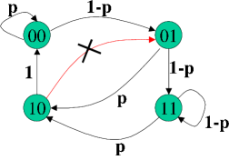
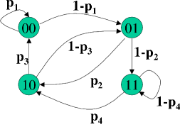
Figure 2: (a) Left: Constrained ergodic Markov source (forbidden word = ‘101’). (b) Right: A general 4-state ergodic Markov source. Note: The case $p_{1}=p_{2}=p_{3}=p_{4}=p$ yields an i.i.d source and the case $p_{1}=p_{2}=p_{4}=p,p_{3}=1$ yields the source with forbidden word ‘101’. Thus the general 4-state ergodic Markov source captures both cases.

4.1 Constrained Ergodic Markov Sources

We shall model constrained sources as a Markov source. In this paper, we shall consider only those Markov sources that are ergodic. A Markov source is ergodic if either the Markov chain itself is ergodic [9] or equivalently, the dynamical system in which the Markov chain is embedded is ergodic. We know by the theory of Markov chains [9] that all finite discrete time Markov chains that are ergodic (i.e. they are irreducible and aperiodic) have an unique stationary distribution, also known as invariant distribution. This means that given any arbitrary initial distribution on the Markov states, it eventually settles to an unique probability distribution. Once we have an unique stationary distribution with finite states, Shannon’s entropy rate can be calculated. In general, it is hard to determine the invariant measure of the underlying dynamical system in which the Markov chain is embedded, but it is relatively easy to determine whether the Markov chain is ergodic (all we need to do is test for irreducibility and aperiodicity).

We already saw in Section 2 how an i.i.d source $X$ can be seen as a 0-order Markov chain with finite number of states. We could do similarly for ergodic Markov sources. As an example, a binary ergodic Markov source with ‘101’ as a forbidden word is shown in Figure 2.

4.2 Computing Shannon’s entropy rate

In Figure 2, a general four state Markov source is also shown. The condition $p_{1}=p_{2}=p_{3}=p_{4}=p$ implies that the source is i.i.d. The condition $p_{1}=p_{2}=p_{4}=p$ and $p_{3}=1$ corresponds to the ergodic Markov source with the forbidden word ‘101’. We shall deal with the general four state Markov source (assuming that it is ergodic).

The transition probability matrix for the general four state ergodic Markov source is given by:

$$P=\begin{bmatrix}p_{1}&1-p_{1}&0&0\\ 0&0&p_{2}&1-p_{2}\\ p_{3}&1-p_{3}&0&0\\ 0&0&p_{4}&1-p_{4}\\ \end{bmatrix}.$$

The unique stationary probability distribution $\Pi$ (a row vector of dimension $1\times|\mathcal{A}|$) can be determined by solving the equation:

$$\Pi P=P.$$ (1)

Since $P$ is always a stochastic matrix (every row adds to 1) of dimension $|\mathcal{A}|\times|\mathcal{A}|$, there exists a unique eigenvector $\Pi$ for $P$ corresponding to the eigenvalue 1. We normalize $\Pi$ as follows:

$$\hat{\Pi}=\frac{\Pi}{\|\Pi\|}.$$ (2)

Once we have $\hat{\Pi}=\{\Phi_{1},\Phi_{2},\ldots,\Phi_{|\mathcal{A}|}\}$ we can compute Shannon’s entropy of the source $X$ as follows:

$$H_{X}=-\frac{1}{log_{2}(Num)}\sum_{i=1,\Phi_{i}\neq 0}^{i=|\mathcal{A}|}\Phi_{i}log_{2}(\Phi_{i}).$$ (3)

The units of $H_{X}$ is bits/symbol and $Num$ represents the number of Markov states. For the general 4-state ergodic Markov source, this will be 1/2 since each states accounts for 2 bits of the message.

4.3 Modified GLS-coding

In this section, we shall embed the general 4-state ergodic Markov source into a non-linear dynamical system. We shall determine the initial condition for any given symbolic sequence (message) on the resulting dynamical system and use the initial condition to compress the message (similar to GLS-coding). We shall show that such a method achieves Shannon’s entropy rate $H_{X}$.

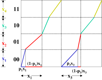
Figure 3: Embedding a constrained ergodic Markov source in a dynamical system with the map $T$: [0,1) $\mapsto$ [0,1).

4.4 Embedding

We shall embed the general 4-state ergodic Markov source into a non-linear dynamical system similar to GLS for the i.i.d source. To each Markov state, we associate a Markov partition of the dynamical system (refer to Figure 3). We want the messages of this source to be symbolic sequences of the dynamical system. Draw straight lines with slopes yet to be determined connecting those states that communicate. For example, 00 communicates only with 01 and 10. Let the lengths of the Markov paritions be $x_{1}$, $x_{2}$, $x_{3}$ and $x_{4}$. We then write the “measure-preserving” constraints as follows:

$$p_{1}x_{1}+p_{3}x_{3} = x_{1}~{}~{}~{}(for~{}~{}00)$$

$$(1-p_{1})x_{1}+(1-p_{3})x_{3} = x_{2}~{}~{}~{}(for~{}~{}01)$$

$$p_{2}x_{2}+p_{4}x_{4} = x_{3}~{}~{}~{}(for~{}~{}10)$$

$$(1-p_{2})x_{2}+(1-p_{4})x_{4} = x_{4}~{}~{}~{}(for~{}~{}11)$$

These constraints automatically satisfy $x_{1}+x_{2}+x_{3}+x_{4}=1$. Solving the first two of the above equation yields $x_{3}=x_{2}$. The above linear set of equations can be solved for the given set of $\{p_{1},p_{2},p_{3},p_{4}\}$ (if the Markov chain is ergodic, a unique solution always exists). The solution gives the length of the Markov partitions $\{x_{1},x_{2},x_{3},x_{4}\}$ which is unique. The slopes of the line segments are determined from the probabilities. We thus have a dynamical system (modified GLS) and we shall show that this embeds the ergodic Markov source.

4.5 Interpretation of the “measure-preserving” constraints

How do we understand the “measure-preserving” constraints? As an example, consider the Markov partition of length $x_{1}$ corresponding to the state 00. Since 00 communicates only with itself and 01, we have the range of the function limited to intervals 00 and 01. The slope of the line segment (in blue) which maps fraction of $x_{1}$ to 00 is $\frac{1}{p_{1}}$. This is because whenever we are in state 00, the probability that we end up in the same state on receiving the next symbol is $p_{1}$. Thus $p_{1}x_{1}$ is the fraction of initial conditions which end up in the same state 00. The remaining $(1-p_{1})x_{1}$ fraction of initial conditions end up in 01. Similarly, we do this for all the states. The “measure-preserving” constraint for say the state 00 is indicating what fraction of initial conditions end up in state 00 in one iteration. This is formed precisely as the sum of the fraction $p_{1}x_{1}$ which come from 00 and $p_{3}x_{3}$ that comes from 10 (because these are the only two states that communicate with 00). This is how we get all the constraint equations.

4.6 “Measure-preserving” constraints are equivalent to $\Pi P=P$.

The linear set of “measure-preserving” constraints can be written in matrix form as follows:

$$\begin{bmatrix}x_{1}&x_{2}&x_{3}&x_{4}\\ \end{bmatrix}\begin{bmatrix}p_{1}&1-p_{1}&0&0\\ 0&0&p_{2}&1-p_{2}\\ p_{3}&1-p_{3}&0&0\\ 0&0&p_{4}&1-p_{4}\\ \end{bmatrix}=\begin{bmatrix}x_{1}&x_{2}&x_{3}&x_{4}\\ \end{bmatrix}.$$

Notice that the above equation is the same as $\Pi P=P$ where $P$ is the transition probability matrix of the Markov source. Thus $\{x_{1},x_{2},x_{3},x_{4}\}$ is nothing but the unique stationary probability distribution obtained from the equation $\Pi P=P$.

We have thus embedded the ergodic Markov source in to a non-linear dynamical system.

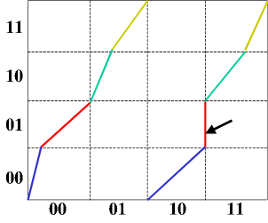
Figure 4: Embedding for the source with forbidden word ‘101’. Notice how one of the slope becomes infinite since ‘10’ is forbidden to communicate with ‘01’.

4.7 Modified GLS-coding achieves Shannon’s entropy rate

In order to prove that encoding the initial condition on the modified GLS will achieve Shannon’s entropy rate, we compute the Lyapunov exponent of the modified GLS and show that this is the same as Shannon’s entropy rate. In fact, the non-linear dynamical system is a faithful modelling of the general 4-state ergodic Markov source.

It is important to observe that the modified GLS shown in Figure 3 does not preserve the Lebesgue measure. However, if we restrict all the intervals on the y-axis to strictly lie in one of the four intervals labelled 00, 01, 10 and 11 only, then we see that the Lebesgue measure (=probability measure) is actually preserved (sum of the measures of all the inverse images of a particular interval on the y-axis is equal to the measure of that interval we started with). In fact, this is what we ensured by the “measure preserving” constraints in the first place. We could hence compute the Lyapunov exponent as if the map preserved the Lebesgue measure everywhere.

Computation of Lyapunov exponents is then straightforward and yields the following expression (the base of the logarithm in all our Lyapunov exponent computation is always 2, though the standard practice is to use $e$.)

$$\lambda=-\sum_{i=1}^{4}p_{i}log_{2}(p_{i})=2H_{X}.$$

This is nothing but twice the Shannon’s entropy rate $H_{X}$ of the source. The factor 2 is because in every iteration, the symbolic sequence emitted by the source consists of two symbols. Thus, we have faithfully modelled the general 4-state ergodic Markov source as a non-linear dynamical system. Hence modified-GLS coding would achieve the Shannon’s entropy rate and is optimal for compression.

5 Conclusions and Future Research Directions

In this paper, we have shown how one can embed an i.i.d source in to a non-linear dynamical system, namely Generalized Luröth Series or GLS. We then considered Markov sources which are not independent anymore. Constrained sources were defined as ergodic Markov sources with certain forbidden words. We showed how to compute the Shannon’s entropy rate and also modified GLS to compresses messages from these sources. The modified-GLS is a faithful embedding of constrained sources and hence achieves Shannon’s entropy rate.

It is possible to generalize our method for a list of arbitrary forbidden words. Implementation issues were not discussed in this paper. It may be worthwhile to investigate joint compression and encryption for constrained sources.

References

- [1] K. Sayood, Introduction to Data Compression, Morgan Kaufmann (1996)
- [2] C.E. Shannon, A Mathematical Theory of Communication, Bell Sys. Tech. J. 27 (1948) 379–423.
- [3] D. Salomon, Data Compression: The Complete Reference, Springer-Verlag, New York (2000).
- [4] D.A. Huffman, A method for the construction of minimum-redundancy codes, Proceedings of the I.R.E. (1952) 1098–1102.
- [5] N. Nagaraj, P.G. Vaidya, K.G. Bhat, Joint Entropy Coding and Encryption using Robust Chaos, arXiv.org:nlin.CD/0608051 (2006).
- [6] P.G. Vaidya, N. Nagaraj, Foundational Issues of Chaos and Randomness: “God or Devil, Do We Have A Choice?”, Proc. of Foundations of Sciences, Project of History of Indian Science, Philosophy and Culture New Delhi (2006).
- [7] K.T. Alligood, T.D. Sauer, J.A. Yorke, Chaos: An Introduction to Dynamical Systems, Springer, New York (1996).
- [8] K. Dajani, C. Kraaikamp, Ergodic Theory of Numbers, 29. Mathematical Association of America, Washington, DC (2002).
- [9] S.P. Meyn, R.L. Tweedie, Markov Chains and Stochastic Stability, Springer-Verlag (1993).