A radiative transfer scheme for cosmological reionization based on a local Eddington tensor.

Abstract

A radiative transfer scheme is presented, based on a moment description of the equation of radiative transfer and the so–called “M1 closure model” for the Eddington tensor. This model features a strictly hyperbolic transport step for radiation : it has been implemented using standard Godunov–like techniques in a new code called ATON. Coupled to simple models of ionization chemistry and photo-heating, ATON is able to reproduce the results of other schemes on a various set of standard tests such as the expansion of a HII region, the shielding of the radiation by dense clumps and cosmological ionization by multiple sources. Being simple yet robust, such a scheme is intended to be naturally and easily included in grid–based cosmological fluid solvers.

1 Introduction

During the early stages of the Universe, the process of structure formation leads to the formation of the first stars at a redshift $z\sim 10-20$. These primordial, metal-poor stars should emit a substantial amount of radiation that would be able to ionize the neutral gas that fills the surrounding space (see e.g. Barkana & Loeb (2001) for an extensive review). Afterward, it would become transparent to radiation at high energies, where the transition is commonly pictured as ionized bubbles that expand and percolate around sources. The investigation of the the distribution of neutral gas at high redshift is therefore a great source of knowledge on the first luminous objects, on the physical conditions in which they appear and on the cosmological context that lead to them. For this purpose, several experiments were or are about to be set up : one can mention LOFAR or SKA which aim at detecting the redshifted 21 cm signal which would come up from the neutral hydrogen.

From a theoretical point-of-view, the interest of pursuing so-called ’full-physics’ cosmological simulations has been recently emphasized by different groups These numerical experiments can predict the history of star formation, the large scale gas distribution hosting small scale disc–like objects, the creation and ejection of metals, etc… While intensively tested at low redshift, only a few observational comparisons are available for $z>3$ and basically none for $z>5$. In this context, the comparison of simulations’ prediction to the observed 21 cm emission would open a new range of epochs during which the understanding of the formation of structures could be tested.

Common features of hydrodynamical simulations are gravity, hydrodynamics and star formation. They are modeled self-consistently and coupled to each other, up to a certain extent. On the other hand, the radiation is often considered as an external homogeneous background and its impact on the physics is not exactly consistent with the distribution of sources inside the simulated box. A common approach consists in taking in account a diffuse radiation background which evolves along time according to a model of cosmological radiation sources ( see e.g. Madau et al. (1999)). The geometrical distribution of the sources and the propagation of the emitted radiation in the neutral hydrogen gas cannot be eluded if one is interested in the transition processes that occur at the reionization. Note that still at lower redshift, although the universe is fully ionized, the radiation field is still highly inhomogeneous down to redshift 1 ( see e.g. Madau et al. (1999)).

A great effort has been put into developing tools that simulate the emission and the propagation of radiation in cosmological boxes and its impact on the gas physics through heating/cooling processes and ionization (see e.g. Gnedin & Abel (2001), Mellema et al. (2006)). A perfect illustration of this interest in given by Iliev et al. (2006) where a large number of radiative transfer codes were gathered in order to be tested on the same set of numerical experiments. Several methods (ray shooting, grid-based codes, Monte-Carlo) and several types of implementation (post-processing, self-consistent simulations) are compared and this project demonstrates that different methods can achieve very similar results even though they greatly differ in their conception. We would like to stress here that in this comparison paper, only one moment–based code was used, namely the OTVET code (Gnedin & Abel, 2001), and its use was only restricted to strictly periodic problems.

In this paper, we present a new moment–based method to perform calculations of radiative transfer. It relies on a rather standard hyperbolic grid–based solver and is simple enough to be quickly implemented. This method relies on a momentum description of the transfer equation via the conservation of radiative energy and flux. Gnedin & Abel (2001) relied on the same type of description of the equation of radiative transfer, where the Eddington’s tensor is constrained by the sources’ geometry, assuming an optically thin regime. We use here to compute the Eddington tensor the so–called M1 closure relation, which provides a variable Eddington tensor that depends only on the local radiation flux and intensity. Non-equilibrium ionization is also taken in account by solving the coupled set of equations for out–of–equilibrium hydrogen chemistry. The current implementation performs only post-processing of existing simulation, even though it can in principle be easily coupled to a grid-based hydrodynamical code.

The paper is organized as follows: the first section briefly introduces the model. The numerical implementation is then presented in more details. The third section is devoted to the same tests performed in Iliev et al. (2006), on rather academic situations but also on realistic cosmological fields. The range of applications of this new scheme is discussed in the last section.

2 Radiative transfer as an hyperbolic system of conservation laws with source terms

The current scheme is based on a momentum description of the radiative transfer equation. The hierarchy of equations is truncated at the second order and the closure relation is provided by the M1 relation.

2.1 Moments of the transfer equation

The radiative transfer equation is given by:

$$\frac{1}{c}\frac{\partial I_{\nu}}{\partial t}+{\bf n}\cdot{\bf\nabla}I_{\nu}=-\kappa_{\nu}I_{\nu}+\eta_{\nu},$$ (1)

where $I_{\nu}({\bf x},{\bf n},t)$ is the radiation specific intensity, $\kappa_{\nu}({\bf x},{\bf n},t)$ the absorption coefficient and $\eta_{\nu}({\bf x},{\bf n},t)$ the source function. They all depend on position, angle, frequency and time. The absorption coefficient, in the context of ionizing radiation, is computed from

$$\kappa_{\nu}=n_{\rm H_{0}}\sigma_{\nu},$$ (2)

where $\sigma_{\nu}$ is the photoionization cross section, and $n_{\rm H_{0}}$ the neutral hydrogen density. By taking the first two momenta of Eq. 1, two coupled equations can be obtained:

$$\frac{\partial E_{\nu}}{\partial t}+\nabla{\bf F}_{\nu} = -\kappa_{\nu}cE_{\nu}+S_{\nu},$$ (3)

$$\frac{\partial{\bf F}_{\nu}}{\partial t}+c^{2}\nabla{\bf P}_{\nu} = -\kappa_{\nu}c{\bf F}_{\nu}.$$ (4)

These four equations set the conservation of the radiative energy $E_{\nu}$, the zero-th order momentum of the intensity, and the conservation of the radiative flux ${\bf F}_{\nu}$, the first order momentum. The lower dimensionality of these equations, plus their conservative form, make them more suited to a numerical treatment. However, an expression for the pressure tensor ${\bf P}_{\nu}$ (i.e. the second order momentum of the intensity) must be provided in order to close the system described by Eqs. 3 and 4. This issue is addressed in Sec. 2.4.

From now on, Eq. (3) and Eq. (4) can be modified in a form more suitable to the subsequent calculations. First, the energy and flux densities can be replaced by number densities : this is easily achieved by dividing Eq. (3) and Eq. (4) by a single photon energy, $h\nu$. They become :

$$\frac{\partial N_{\nu}}{\partial t}+\nabla{{\bf F}}_{\nu} = -\kappa_{\nu}cN_{\nu}+S_{\nu},$$ (5)

$$\frac{\partial{{\bf F}}_{\nu}}{\partial t}+c^{2}\nabla{{\bf P}}_{\nu} = -\kappa_{\nu}c{{\bf F}_{\nu}},$$ (6)

where $N_{\nu}$ is the photon number density. For sake of simplicity, we have used the same notation for the photon flux (resp. photon pressure tensor) than for the energy flux (resp. energy pressure tensor), although they differ by the factor $h\nu$. The source term is further divided into 2 contributions

$$S_{\nu}=\dot{N}^{*}_{\nu}+\dot{N}^{rec}_{\nu}~{}~{}~{}{\rm where}~{}~{}~{}\dot{N}^{rec}_{\nu}=n_{\rm e}n_{\rm H_{+}}\dot{\epsilon}_{\nu}(T)$$ (7)

where the first term is the radiation coming from stars or quasars and the second term is the diffuse radiation due to recombination from $\rm H_{+}$ . Both radiation sources are assumed to be isotropic, so that no source term appears in the flux equation. In the test section, we will compare our method to ray–tracing schemes developed in the context of cosmological reionization (Iliev et al., 2006), for which recombination radiation is emitted along each ray, so that recombination radiation is not isotropic anymore. In order to mimic the effect of ray–tracing, we optionally solve a modified equation for the flux

$$\frac{\partial{{\bf F}}_{\nu}}{\partial t}+c^{2}\nabla{{\bf P}}_{\nu} = -\kappa_{\nu}c{{\bf F}_{\nu}}+\frac{\dot{N}^{rec}_{\nu}}{N_{\nu}}{\bf F}_{\nu}.$$ (8)

We call this approximation the “ray–tracing scheme”, although the underlying method still makes use of the 2 first moments of the radiative transfer equation.

2.2 Single group radiative transfer

In the current implementation of ATON, we have restricted ourselves to the ionization of a single specie, namely hydrogen, and discard completely the fate of helium and other elements. It is relatively straightforward to extend our scheme to a more realistic chemical composition, using for example the multiple–frequency approach described in Gnedin & Abel (2001). This is beyond the scope of this paper. We further simplify the problem by considering only one photon group, namely all photons with energy greater than the threshold energy for hydrogen. We use throughout this paper the notations introduced by Katz et al. (1996). The number density of hydrogen nuclei is $n_{\rm H}=\rho X/m_{p}$ (for which we adopt $X=0.76$), while the number density for neutral hydrogen (resp. ionized hydrogen) is noted $n_{\rm H_{0}}$ (resp. $n_{\rm H_{+}}$).

We define the ionizing photons number density as

$$N_{\gamma\rm H_{0}}=\int^{\infty}_{\nu_{\rm H_{0}}}N_{\nu}{\mathrm{d}}\nu.$$ (9)

Integrating Eq. (5) and Eq. (6) over photon frequency and dropping the subscript $\rm H_{0}$ since we have only one photon group in this paper, we get

$$\frac{\partial N_{\gamma}}{\partial t}+\nabla{\bf F}_{\gamma} = -n_{\rm H_{0}}c\sigma_{N}N_{\gamma}+\dot{N}^{*}_{\gamma}+\dot{N}^{rec}_{\gamma},$$ (10)

$$\frac{\partial{\bf F}_{\gamma}}{\partial t}+c^{2}\nabla{\bf P}_{\gamma} = -n_{\rm H_{0}}c\sigma_{F}{\bf F}_{\gamma},$$ (11)

where we define two frequency–averaged cross–sections given by

$$\sigma_{N}N_{\gamma}=\int^{\infty}_{\nu_{\rm H_{0}}}\sigma_{\nu}N_{\nu}{\mathrm{d}}\nu~{}~{}~{}\rm{and}~{}~{}~{}\sigma_{F}F_{\gamma}=\int^{\infty}_{\nu_{\rm H_{0}}}\sigma_{\nu}F_{\nu}{\mathrm{d}}\nu.$$ (12)

In order to simplify further the problem, we assume a simple reference radiation intensity, noted $J_{0}(\nu)$, for which we pre-compute the average cross–section as follows

$$\sigma_{F}\simeq\sigma_{N}\simeq\sigma_{\gamma}=\int^{\infty}_{\nu_{\rm H_{0}}}\sigma_{\nu}\frac{4\pi J_{0}(\nu)}{h\nu}{\mathrm{d}}\nu~{}/\int^{\infty}_{\nu_{\rm H_{0}}}\frac{4\pi J_{0}(\nu)}{h\nu}{\mathrm{d}}\nu,$$ (13)

where the hydrogen photoionization cross–section $\sigma_{\rm H_{0}}(\nu)$ is taken from Hui & Gnedin (1997). Except in section 4.1, we will consider $10^{5}$ K black-body models where $\sigma_{\gamma}=1.63\times 10^{-18}$ cm². Likewise, the recombination radiation, integrated over frequency in our single energy group writes

$$\dot{N}^{rec}_{\gamma}=\int^{\infty}_{\nu_{\rm H_{0}}}n_{\rm e}n_{\rm H_{+}}\dot{\epsilon}_{\rm H_{+}}(\nu,T)=n_{\rm e}n_{\rm H_{+}}(\alpha_{A}-\alpha_{B}).$$ (14)

where $\alpha_{A}(T)$ (resp. $\alpha_{B}(T)$) is the case A (resp. case B) recombination coefficient for $\rm H_{+}$. They are both taken from from Hui & Gnedin (1997). The set of equations we solve in this paper is finally :

$$\frac{\partial N_{\gamma}}{\partial t}+\nabla{\bf F}_{\gamma}=-n_{\rm H_{0}}c\sigma_{\gamma}N_{\gamma} + n_{\rm e}n_{\rm H_{+}}(\alpha_{A}-\alpha_{B})$$ (15)

$$+ \dot{N}^{*}_{\gamma},$$

$$\frac{\partial{\bf F}_{\gamma}}{\partial t}+c^{2}\nabla{\bf P}_{\gamma}=-n_{\rm H_{0}}c\sigma_{\gamma}{\bf F}_{\gamma}.$$ (16)

Let us recall that this set of equation is obtained for one single group of photons, the ionizing ones. The same procedure can be applied in principle to an arbitrary number of groups, in order to achieve a better spectral description of the problem. The number of systems to be solved would therefore scale with the number of groups considered.

2.3 Hydrogen thermochemistry

In order to close the last system of equation, we need to solve for the time evolution of the Hydrogen ionization fraction and of the gas temperature. The chemical evolution of neutral hydrogen is governed by a delicate balance between collisional ionization, photoionization and collisional recombination. These processes are part of the following evolution equation for $n_{\rm H_{0}}$

$$\frac{\rm D~{}}{\rm Dt}(n_{\rm H_{0}})=\alpha_{A}n_{\rm e}n_{\rm H_{+}}-\beta n_{\rm e}n_{\rm H_{0}}-\Gamma_{\gamma\rm H_{0}}n_{\rm H_{0}},$$ (17)

together with charge conservation $n_{\rm e}=n_{\rm H_{+}}$ and Hydrogen nuclei conservation $n_{\rm H_{+}}+n_{\rm H_{0}}=n_{\rm H}$. $\Gamma_{\gamma\rm H_{0}}$ is the Hydrogen atom photoionization rate, given by (using the same notations as for Eq. 12)

$$\Gamma_{\gamma\rm H_{0}}=c\sigma_{\gamma}N_{\gamma}.$$ (18)

Radiative cooling and photoionization heating are also self–consistently taken into account by solving the gas thermal energy equation

$$\rho\frac{\rm D~{}}{\rm Dt}(\frac{e}{\rho})={\cal H}-{\cal L},~{}~{}~{}{\rm with}~{}~{}~{}e=\frac{3}{2}n_{\rm tot}k_{B}T.$$ (19)

The cooling rate, $\cal L$, in erg/s/cc, is computed using standard collisional cooling processes due to case A and B recombination of Hydrogen, collisional ionization and excitation of Hydrogen and Bremsstrahlung. We use the cooling rates given by Hui & Gnedin (1997), Maselli et al. (2003) and references therein. The photoionization heating rate, $\cal H$, also in erg/s/cc, is given by ${\cal H}=n_{\rm H_{0}}\dot{\epsilon}_{\rm H_{0}}$ where

$$\dot{\epsilon}_{\rm H_{0}}=c\int_{\nu_{\rm H_{0}}}^{\infty}(h\nu-h\nu_{\rm H_{0}})\sigma_{\nu}N_{\nu}{\mathrm{d}}\nu=c\epsilon_{\gamma}\sigma_{\gamma}N_{\gamma}.$$ (20)

Following the approach used in the last section, we approximate this photoionization energy using the fiducial $10^{5}$ K black body radiation spectrum, so we can precompute the average photon energy $\epsilon_{\gamma}$ (equals to 29.65 eV in this case).

2.4 The M1 closure relation

As already mentioned, we need to specify the form of the Eddington tensor in order to close the moment hierarchy and solve the previous set of equations. Gnedin & Abel (2001) suggested to compute the Eddington tensor assuming an optically thin medium and summing up the contribution of all the background sources. In this way, the radiative intensity geometry was fully specified and the moment equations could be solved. This techniques, refereed to as the “Optically Thin Variable Eddington Tensor” method, required to solve four different Poisson-like equations. Since all cosmology codes already have a Poisson solver to compute the dark matter and gas dynamics, this scheme turned out to be quite efficient and accurate for cosmological applications. In this paper, we propose to apply a very simple closure relation to cosmological reionization, called the “M1 approximation”, introduced more than two decades ago to solve the radiative transfer equations in the optically thick limit, while retaining some accuracy in the optically thin regime (Levermore, 1984).

It relies on the assumption that the radiation angular distribution is axysymetric around the flux vector ${\bf F}$, so that the Eddington tensor, defined as ${\bf P}={\bf D}N$, can be written in the general form:

$${\bf D}=\frac{1-\chi}{2}{\bf I}+\frac{3\chi-1}{2}{\bf u}\otimes{\bf u},$$ (21)

where ${\bf u}$ is a unit vector aligned with the flux direction. We need also th define the reduced flux $\bf f$ by:

$${\bf f}=\frac{{\bf F}}{cN}=f{\bf u}.$$ (22)

The Eddington factor $\chi$ is a yet unknown scalar quantity that depends only on $f$, and that should satisfy $1/3\leq\chi\leq 1$. We now need a model to specify the functional form for $\chi(f)$. In his review paper, Levermore (1984) discussed a great variety of closure relations. The most simple and physically meaningful one is called the M1 model, for which we have:

$$\chi=\frac{3+4|{\bf f}|^{2}}{5+2\sqrt{4-3|{\bf f}|^{2}}}.$$ (23)

This closure relation corresponds to the angular distribution of a Lorentz boosted isotropic distribution (Levermore, 1984), as for the Cosmic Microwave Background dipole, for which the boost direction is aligned with the flux vector. It has been shown by Dubroca & Feugeas (1999) that this closure relation is the only one that minimize the radiative entropy.

This closure relation is of course a very crude approximation of the true radiation distribution. In presence, for example, of two distinct radiation source, the M1 model will replace the two sources by one “average” source in between. Nevertheless, this colure relation has good properties that we now discuss in more details. This model satisfies the physical constraint $1/3\leq\chi\leq 1$. The tensor ${\bf D}$, which describes the radiation’s local geometry, consists in two separate contributions. The first one is an isotropic component, where the radiation affects all the directions in a similar way. In Eq. 21, the second tensor component of ${\bf D}$ exhibits principal directions that are aligned with the local flux, consistently with a free-streaming radiation. On the one hand, the isotropic component disappears in a pure transport regime with $f=1$, i.e. $\chi=1$. On the other hand, the diffusion regime implies $f=0$ and $\chi=1/3$. Using this value in Eq. 21 shows that only the isotropic component remains, as expected. In a general fashion, all the intermediate regimes represent local geometries where both an isotropic radiation and a free-streaming radiation contribute. These two limiting cases are exactly described by the M1 model, while the general regimes are approximated by a linear combination of these two limiting cases.

The other interesting property is that this model is purely local, so that no expensive Poisson solvers are necessary. Even more interestingly, it can be shown that the left-hand side of Equations (15) and (16) defines an hyperbolic system of conservation laws, with real eigenvalues corresponding to waves traveling at (or close to) the speed of light. (Dubroca & Feugeas, 1999; González et al., 2007). We can therefore use standard numerical techniques designed in the general framework of hyperbolic conservation laws (Toro, 1999) and apply them to cosmological reionization.

3 Numerical implementation

We now describe in details the numerical scheme we have designed to solve the previous set of equations. We use the classical “operator splitting” approach, decomposing the equations into several steps that are solved in sequence. In the first step, called the “stellar source step”, we add all ionizing photons coming from stellar sources in the radiation field. In the second step, called the “transport step”, we solve the hyperbolic system of conservation laws described in the last section. In the last step, called the “thermochemical step”, we solve the right-hand side of our radiation transport model, together with the evolution of neutral hydrogen density and gas temperature.

For the first step, we perform in each cell of the computational grid, indexed $i$, the following update:

$$\left(N_{\gamma}\right)^{n+1}_{i}=\left(N_{\gamma}\right)^{n}_{i}+\dot{N}^{*}_{\gamma}\Delta t$$ (24)

Here and in the followings, index $n$ stands for the radiation field before the current step, and index $n+1$ for the radiation field after the current step. Since we have three intermediate steps, if we start a given time $t$ with index $n$, we reach the next time step at time $t+\Delta t$ with index $n+3$.

3.1 Transport Step

The next operator we solve in our sequence is the hyperbolic system we have discussed in the next section:

$$\frac{\partial N_{\gamma}}{\partial t}+\nabla{\bf F}_{\gamma}=0,$$ (25)

$$\frac{\partial{\bf F}_{\gamma}}{\partial t}+c^{2}\nabla{\bf P}_{\gamma}=0,$$ (26)

In ATON, these equations can be solved either implicitly or explicitly, with the following integral form of the conservation laws (expressed here in 1D for sake of simplicity):

$$\frac{\left(N_{\gamma}\right)^{n+1}_{i}-\left(N_{\gamma}\right)^{n}_{i}}{\Delta t}+\frac{\left(F_{\gamma}\right)^{m}_{i+1/2}-\left(F_{\gamma}\right)^{m}_{i-1/2}}{\Delta x} = 0,$$ (27)

$$\frac{\left(F_{\gamma}\right)^{n+1}_{i}-\left(F_{\gamma}\right)^{n}_{i}}{\Delta t}+c^{2}\frac{\left(P_{\gamma}\right)^{m}_{i+1/2}-\left(P_{\gamma}\right)^{m}_{i-1/2}}{\Delta x} = 0.$$ (28)

The flux function ${\cal F}=(F_{\gamma},P_{\gamma})^{T}$ is evaluated at the intercell faces, indexed $i+1/2$, and at time $m$, with $m=n$ for an explicit scheme, whose stability condition imposes a strong constraint on the time step, or with $m=n+1$ for an implicit scheme, unconditionnaly stable. Following González et al. (2007), we compute the intercell flux using standard methods designed for computational fluid dynamics such as the Godunov method or, more generally, such as the class of upwind schemes. If we note ${\cal U}=(N_{\gamma},F_{\gamma})^{T}$ the vector of state variable, the intercell flux depends on the left and right states with respect to the interface:

$${\cal F}^{m}_{i+1/2}={\cal F}({\cal U}^{m}_{i},{\cal U}^{m}_{i+1})$$ (29)

González et al. (2007) have tested various flux functions with respect to the M1 model, and came up with two possibilities, namely the Harten–Lax–van Leer (HLL) flux function, for which we have:

$$\left({\cal F}_{HLL}\right)^{m}_{i+1/2}=\frac{\lambda^{+}{\cal F}^{m}_{i}-\lambda^{-}{\cal F}^{m}_{i+1}+\lambda^{+}\lambda^{-}({\cal U}^{m}_{i+1}-{\cal U}^{m}_{i})}{\lambda^{+}-\lambda^{-}},$$ (30)

where $\lambda^{+}=\max(0,\lambda_{max})$ and $\lambda^{-}=\min(0,\lambda_{min})$ are the maximum and minimum eigenvalues of the Jacobian matrix of the system evaluated at the $i$-th and $i+1$-th cells (for more details, the reader is encouraged to read González et al. (2007)) and the Global Lax Friedrich (GLF) flux function for which the maximum wave speed is taken equal to the speed of light:

$$\left({\cal F}_{GLF}\right)^{m}_{i+1/2}=\frac{{\cal F}^{m}_{i}+{\cal F}^{m}_{i+1}}{2}-\frac{c}{2}({\cal U}^{m}_{i+1}-{\cal U}^{m}_{i}).$$ (31)

As we will demonstrate in the test section, the GLF flux, more diffusive by nature, turns out to give results very similar to the HLL flux, while being much simpler to implement, since it does not require to determine the eigenvalues of a rather complex hyperbolic system.

3.2 Implicit versus explicit ?

The time step of our scheme, $\Delta t$, is controlled by the Courant condition, which writes $3c\Delta t/\Delta x<1$, if the integration is performed explicitly ($m=n$). In cosmological problems, this can result into very small time steps, although the overall solution evolves quite slowly. The standard solution is to use larger time steps, related for example to the much lower ionization front typical propagation speed, but we must rely on implicit integration, for which $m=n+1$. In the latter case, we fix the Eddington factor $\chi$ and the various eigenvalues $\lambda$ to their initial value (index $n$), so that the implicit form of our solver becomes a linear system, as can be seen from Equations (21), (27) and (28). This linear system is then solved using standard sparse solvers, among which the Gauss–Seidel solver gave the best results.

Another alternative to overcome the limitation of the explicit scheme, while avoiding the complexity of the implicit scheme, was proposed by Gnedin & Abel (2001): the “Reduced Speed–of–Light Approximation”. The idea is to replace the actual speed–of–light $c$ by an effective speed–of–light $\tilde{c}\ll c$ in all the previous equations (including the photoionization rates), where $10^{-3}<\tilde{c}/c<1$ is typically considered. By reducing the speed-of-light, the Courant condition becomes looser and larger time steps can be considered. Even though it introduces an approximation, no consequences is found as long as phenomena where the actual speed of propagation remains smaller than $\tilde{c}$ are considered, like the expansion of an HII region. As shown in the following, using $\tilde{c}$ instead of $c$ has no consequence on the accuracy of the results. Furthermore, there are also a significant number of cases where satisfying the strict Courant condition can be handled numerically, still avoiding the rather costly implicit solver. In this paper, we have never used the implicit scheme, although in other physical conditions, using the implicit solver can be unavoidable.

3.3 Thermochemical step

In our operator splitting approach, the last step solves for the chemical evolution of Hydrogen and for the coupling between radiation and matter. Physical quantities such as the gas temperature or the ionization fraction must be updated. The equations we solve here are the followings:

$$\frac{\partial N_{\gamma}}{\partial t} = -n_{\rm H_{0}}c\sigma_{\gamma}N_{\gamma}+n_{\rm e}n_{\rm H_{+}}(\alpha_{A}-\alpha_{B})$$ (32)

$$\frac{\partial{\bf F}_{\gamma}}{\partial t} = -n_{\rm H_{0}}c\sigma_{\gamma}{\bf F}_{\gamma}$$ (33)

$$\frac{\partial n_{\rm H_{0}}}{\partial t} = -n_{\rm H_{0}}c\sigma_{\gamma}N_{\gamma}+n_{\rm e}n_{\rm H_{+}}\alpha_{A}-n_{\rm e}n_{\rm H_{0}}\beta,$$ (34)

$$\frac{\partial e}{\partial t} = n_{\rm H_{0}}c\sigma_{\gamma}\epsilon_{\gamma}N_{\gamma}-n_{\rm H_{0}}n_{e}\Lambda_{e{\rm H_{0}}}-n_{\rm H_{+}}n_{e}\Lambda_{e{\rm H_{+}}}.$$ (35)

In these equations, the coefficients $\alpha_{A}$, $\alpha_{B}$, $\Lambda_{e{\rm H_{0}}}$ and $\Lambda_{e{\rm H_{+}}}$ all depend non–linearly on the gas temperature. The various chemical species’ densities can be expressed as a function of the ionization fraction $x$ as $n_{e}=n_{\rm H_{+}}=xn_{\rm H}$ and $n_{\rm H_{0}}=(1-x)n_{\rm H}$. The gas internal energy is expressed as $e=3/2(1+x)n_{\rm H}k_{B}T$. Because of the very small time scales involved, we solve this system using a fully implicit scheme. The first two equation are linear with respect to their main unknown, so that the implicit discretization can be worked out analytically:

$$\left(N_{\gamma}\right)^{n+1} = \frac{\left(N_{\gamma}\right)^{n}+\Delta tn_{\rm e}^{n+1}n_{\rm H_{+}}^{n+1}(\alpha^{n+1}_{A}-\alpha^{n+1}_{B})}{1+\Delta tn_{\rm H_{0}}^{n+1}c\sigma_{\gamma}},$$ (36)

$$\left({\bf F}_{\gamma}\right)^{n+1} = \frac{\left({\bf F}_{\gamma}\right)^{n}}{1+\Delta tn_{\rm H_{0}}^{n+1}c\sigma_{\gamma}}.$$ (37)

Injecting these equations into the rest of the system leads to an implicit system of 2 coupled non–linear equations to solve for the 2 variables $x^{n+1}$ and $T^{n+1}$. We describe in the Appendix the technical solution we propose to solve this problem. After this final step, we find the new thermochemical state $(x,T)^{n+1}$, and the corresponding new radiation state $(N_{\gamma},{\bf F}_{\gamma})^{n+1}$, at the new time step $t+\Delta t$.

4 Tests and Results

In their cosmological radiative transfer codes comparison project, Iliev et al. (2006) give a set of standard tests that were used to probe the validity of ATON and its implementation. First the expansion of a Stromgren sphere is simulated, then the shadowing of an I-front by a dense clump is discussed, and a first attempt to model the propagation of radiations in a static cosmological field is presented in the end.

4.1 HII region expansion with a constant temperature

Figure 1: Stromgren sphere test. GLF intercell flux has been used for the left panel’s computations, HLL intercell flux has been used for the right panel’s calculation. The lines stand for the ionized fraction profile and the neutral fraction profile, computed at $t=35$ Myr (top row) and t= 500 Myr (bottom row) with a reduced speed of light $\tilde{c}=c/1000$ (dot-dashed line), $\tilde{c}=c/100$ (dotted line) and $\tilde{c}=c/100$ (plain line). Curves are superimposed at t= 500 Myrs.

Figure 2: Stromgren sphere test. The dotted (resp. plain) lines stand for the I-front position at different times (in units of the recombination time), computed with a reduced speed of light $\tilde{c}=c/1000,c/100,c/10$ (resp. dot-dashed, dotted and plain lines). HLL flux calculation is shown on the right panels, GLF flux calculation on the left panels. Bottom rows: ratio of the simulated front position to the analytic value. Top rows: I-front position evolution in units of the box size. The Stromgren radius is 5.4 kpc and the recombination time is 122.4 Myr.

First, the classical situation where a single source emits a ionizing radiation that propagates through the surrounding neutral medium is presented. It results in the classical picture where an ionized sphere , centered on the source, expands at given rate. As the recombination process starts to counter-balance the ionization, the front’s position slows down and even stops, achieving a stationary regime. Assuming the source emits $\dot{N}^{*}_{\gamma}$ ionizing photons per unit time the Stromgren radius, i.e. the stationary radius, is given by:

$$r_{S}=\left(\frac{3\dot{N}^{*}_{\gamma}}{4\pi\alpha_{B}(T)n_{H}^{2}}\right)^{1/3},$$ (38)

where $\alpha_{B}(T)$ stands for the case B recombination rate at a temperature $T$ and $n_{H}$ is the surrounding gas number density. The time evolution of the I-front’s position is given by

$$r_{I}(t)=r_{S}(1-e^{-\frac{t}{t_{r}}})^{1/3},$$ (39)

where $t_{r}$ is the characteristic recombination time given by $1/t_{r}=\alpha_{B}(T)n_{H}$. From Eq. 39, one can see that the expansion slows down for $t\sim t_{r}$.

The setting for the numerical experiment is similar to the one given by Iliev et al. (2006). The source is located at the corner of the simulated box and emits $\dot{N}^{*}_{\gamma}=5\times 10^{48}$ photons per second. The surrounding hydrogen has a number density of $n_{H}=10^{-3}\mathrm{cm}^{-3}$ with an initial ionized fraction $x=1.2\times 10^{-3}$ and its temperature remains fixed, with $T=10^{4}K$ . The simulation is performed on $64^{3}$ grid, with a $6.6$ kpc box size. Reflexive boundary conditions are assumed. The source is switched on at t=0. The results are presented in Figs. 1 and 2.

Fig. 1 shows the profiles of the ionized and neutral fraction computed with the two different types of intercell flux at t=30 Myr and t=500Myr. Clearly the two methods agree for an effective speed of light that varies from $\tilde{c}=0.001c$ to $\tilde{c}=c$. For instance, both methods return an underestimated I-Front position as $\tilde{c}$ is smaller than the physical propagation speed of the front. Conversely, when $\tilde{c}$ is large enough (typically $\tilde{c}\geq 0.01c$), the two fluxes approximations agree and achieve convergence regarding the result. The same calculation is performed in Iliev et al. (2006) and the results shown in Fig. 1 are consistent with the profiles found by the codes that took part to their comparison project.

In Fig. (2), the I-front’s position is compared to the theoretical calculation. From the top panels of Fig. (2), it clearly appears that the current code accurately reproduces the fast expansion of the ionized bubble at early times and the slow down as the I-front position gets closer to the Stromgren radius. At later times, a stationary state is achieved and the I-front stops. Again, the GLF and HLL calculation agrees and return a final radius $4\%$ larger than the theoretical Stromgren radius. The comparison to Iliev et al. (2006) shows that it is consistent with the other types of calculations which tends to overestimate the final radius’ value. The bottom panels show the comparison between the simulated I-Front position and the theoretical one at each time step. Clearly the two types of intercell fluxes (GLF and HLL) return similar results and both present a drift toward greater values of the front position. For t=500 Myr, the discrepancy is $4\%$. Interestingly, this drift is similar for all values of $\tilde{c}$ and the results only differ by the time required for the profile to ’converge’ toward the drift. For instance, the $\tilde{c}=0.001c$ calculation requires $\sim t_{\mathrm{rec}}$ to catch up the main drift, while it is instantaneous for $\tilde{c}=0.1c$. The results found in Iliev et al. (2006) shows a similar behavior.

4.2 HII region expansion with a variable temperature

In the second test, the HII region expansion is investigated while the gas temperature is allowed to vary as a consequence of photoheating. The numerical setup is identical to the previous test with two exceptions. First, the source is now a $10^{5}$ K black body source while the flux of ionizing photons remains unchanged. Second, the initial gas temperature is set to $100$ K and its evolution is modeled according to the Eq. (19). The source is turned on at $t=0$ and the simulation is run over one recombination time with $\tilde{c}=0.1c$.

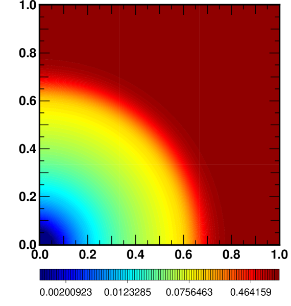
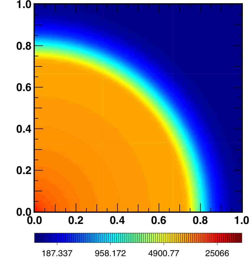
Figure 3: Stromgren sphere test with non uniform temperature. Left : Neutral fraction map in the source plane. Right : temperature (in Kelvin) map in the source plane. These maps were computed 100 Myr after the central source (located here in the bottom left corner) has been switched on. The experimental setting is similar to the constant temperature test, described in section 4.1.

Figure 4: Stromgren sphere test with non uniform temperature. The left panel shows the average temperature profile while the right panel shows the the average ionization and neutral fraction profile. These profiles were computed 10(plain), 35 (dotted) and 100 (dashed-dotted) Myrs after the central source has been switched on. The experimental setting is similar to the constant temperature test, described in section 4.1.

Fig. (3) presents the temperature and neutral fraction maps after 100 Myrs and Fig. (4) presents the time evolution of the temperature and ionized fraction profile. A quick comparison between the constant temperature experiment and the current one indicates that the results qualitatively agrees. For instance, taking the t=35 Myrs profile as a reference, the transition region is in both case located at a radius equals to 0.45 , in units of the box size. However the transition operates on a larger range of radii compared to the isothermal case, the background neutral fraction being achieved at r=0.8 box length at t=35 Myrs while this region does not extend further than r=0.65 in the constant temperature case. This relates to the non-monochromatic source used in the current case : the average photon-energy is larger than previously, hence the average cross-section is diminished and this leads to a smoother transition from the fully ionized to the neutral regime. The temperature profile shows a steady evolution of the limit between the hot medium (T$\geq 10000$K) and the cold neutral medium. The transition between these two regimes is much sharper than observed for the neutral fraction profile. Furthermore the inner temperature profile is practically flat (except close to the center) while the neutral fraction values spans over a few orders of magnitude. It can also be observed on the maps where no dynamics can be seen on the temperature maps while a gradient in the neutral fraction is clearly visible.

Comparisons with Iliev et al. (2006) results show that ATON’s calculations are consistent with other codes, however the transition region’s profile between ionized and neutral gas is sharper in the current calculations than returned by the other codes. It could be related to the current spectral treatment, where a single photon-population (having an energy representative of the source spectrum) is taken in account, the transition’s profile reflecting its typical energy. Conversely, a more complete treatment of spectral hardening is expected to produce smoother profiles, as high-energy photons have larger mean free-path and travel further in the neutral hydrogen.

4.3 Shadowing by a dense clump

The third test investigates the code’s ability to deal with density clumps along the photon’s path. Such clumps are expected to slow down the I-fronts propagation and create regions which are shielded from the radiations due to the shadow trailing behind high density regions. Such situations are likely to happen in a cosmological context where shielding is provided by e.g. gaseous structures or filaments. The setting suggested by Iliev et al. (2006) is adopted: a 6.6 kpc box is considered with a dense and cold clump on the radiation’s path. The background gas density is $\rho=200$ m^-3 with a initial temperature $T=8000$ K. The clump is sphere located at (5, 3.3, 3.3) kpc with a radius $r=0.8$ kpc. Its density is $40000$ m^-3 and its temperature is $T=80$ K. A stationary photon flux $\Phi=10^{10}$m^-3s^-1 photons is ignited at $t=0$ with a typical energy corresponding to a $10^{5}$ K black-body source. Calculations were performed with the HLL intercell flux with $\tilde{c}=c$.

Neutral fraction and temperature maps and profiles are given in Fig. (7) and Fig. (5). Clearly shadows are created in the clump trail: the gas remains neutral behind the clump and its temperature remains lower than the surroundings due to the lack of heating photons in this region. The neutral fraction is almost zero outside the clump due to the incoming flux of photons ad rises to a constant level around $x\sim 0.01$ on the ‘enlightened’ side of the clump as light penetrates the over-density. As illustrated by Fig. (6), the I-front propagates deeper into the clump and after a fast propagation in the optically thin medium, the front almost stops and progress slowly trough the dense medium. On the other hand, the temperature profiles shows a similar behavior with a sharp transition region from $\sim 10500-11000$ K to $80$ K, the initial clump’s temperature. In the ’trailing’ region, temperature is initially lower than in the leading region. However, it is clear from the maps in Fig. (7) that the limits of the trailing shadow are not parallel to the direction of the incident flux, and a diffusion cone appears. As time advances, the temperature in the initially shielded region rises, until it reaches a level close to the one observed in the exposed gas. Finally, Fig. (8) describes the time evolution of the average ionized fraction and temperature inside the clump. Both curves shows a fast increase during the first million years followed by a shallower evolution toward $x=0.8$ and $T=11000$ K. Up to t=10 Myrs, these evolutions are in a quantitative agreement to the ones presented in Iliev et al. (2006), which indicates that the current scheme captures the overall picture of the I-front trapping, even though the lack of multi-frequency treatment leads to some discrepancies in the detailed description of the process.

From a physical point-of-view, a certain level of diffusivity is expected : atoms recombine and radiate in an isotropic fashion. In the current scheme, isotropy is taken in account by the spherical component of the Eddington’s tensor and its relative contribution is set by the ratio of the local flux by the energy ( the reduced flux $f$). From the maps in Fig. (5), the clear conic shape of the trailing shadow appears as a manifestation of this isotropy. However, ATON’s predicts a larger shadow’s extent compared to experiments in Iliev et al. (2006) where it remains parallel and clear cut : this discrepancy is likely to be related to the lack of modelisation of the recombination’s isotropy. As stated in the first section, ATON’s can mimic the behavior of a ray-tracing code by adding an extra artificial term in the flux equation (see Eq. (8) and Eq. (LABEL:e:rt2)). The computations using this scheme are significantly different from the one using the regular scheme and are in good agreement with results shown in Iliev et al. (2006) . In Fig. (7), it clearly appears that the ’ray–tracing’ scheme is much more ’conservative’ in terms of flux geometry: the shadows are clear cut behind the clump. It is particularly striking in the temperature maps where basically no shadow persists after a given duration in the regular calculation while it remains and exhibits sharp edges in the current enhanced calculation. The same effect can be noted in the neutral fraction maps where the cone-shaped shadow is replaced by a straight cylindrical one. It persists over the 15 Myrs of the calculation. In terms of profiles, it can be seen from Fig. (5), Fig. (8) and Fig. (6) that the I-front propagation is affected too and their progression through the clump is faster. The radiation’s flux is more ’rigid’ and the influence of diffusion is lowered : the ionization of a propagating front is more efficient especially in dense regions where I-front can be significantly slowed down. Also, the smaller diffusivity keeps the initial temperature profile in the shielded region unchanged. Let us emphasize that these results are obtained using an artificial flux term and should be considered with caution since diffusivity must appear at some point. As shown hereafter, the differences remain small in realistic cosmological situations but still : in the current setting clear cut shadows are obtained by suppressing the isotropic recombination and as shown in the results obtained using the regular ATON’s scheme, results can be significantly different in certain situations.

The other differences with the calculations presented in Iliev et al. (2006) can be explained by the lack of multi-frequency treatment. Because the scheme do not take in account the effect of high frequency photons with large mean free-path, no preheating on large distance is being modeled. With the current single-energy treatment, the effect of these photons tend to be underestimated and all processes (ionization and photo-heating) occur on small scales, leading to the observed sharp profiles. In Fig. (5) , the ionization fraction transition from ionized background to neutral clump is much sharper in ATON’s case and no steady decrease can be observed. Other codes do not present a sharp drop in ionized fraction and a smoother transition exists between the neutral fraction of the irradiated side to the shielded side. A similar discrepancy exists in the temperature profile, where the drop in temperature occurs on smaller distances. The average ionized fraction within the clump is also a few percent smaller than found in other calculations at late times. In other words, the progression of the I-front within the clump appears to be slightly slower in ATON’s calculations, the trapping is more efficient. It results from the lack of preheating and ionization by high energy photons. In the prospect of cosmological studies, where sources are likely to be embedded in high density regions, the radiation is therefore expected to take a slightly larger amount of time to escape from the haloes in the current scheme compared to other calculations.

Figure 5: Shadowing by a dense clump using HLL intercell flux. Top: Temperature profile along the middle section of the box. Bottom: Neutral and ionized fraction profile along the same section. Profiles were computed at t= 1 (bottom row), 3 (middle row) and 10 (top row) Myrs. The radiation comes from the left side of the maps. Thin solid lines stand for the computation using the ’regular’ M1 scheme while thick dashed lines stand for the computation using our “ray–tracing” scheme.

Figure 6: Shadowing by a dense clump. The I-front position as a function of time for the regular ATON’s scheme (thin solid line) and “ray–tracing” scheme (thick dashed line). The position of the I-front, relative to the clump center is given in units of the Stromgren length defined as $\ell_{S}=F/\rho^{2}\alpha_{B}$.

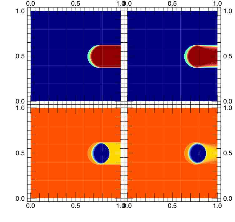
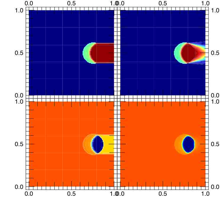
Figure 7: Shadowing by a dense clump using HLL intercell flux. Top: neutral fraction (top row) and temperature map (bottom row) along the middle section of the box, measured at t=1Myr. Bottom: same measurements at t= 3 Myrs. Left columns stand for computations with a “ray–tracing” scheme, while right columns stand for the ’regular’ M1 scheme.

Figure 8: Shadowing by a dense clump. The time evolution of the average ionized fraction (top) and the average temperature (bottom) within the clump for the regular ATON’s scheme (thin solid line) and the “ray–tracing” scheme (thick dashed line).

4.4 Static Cosmological Field

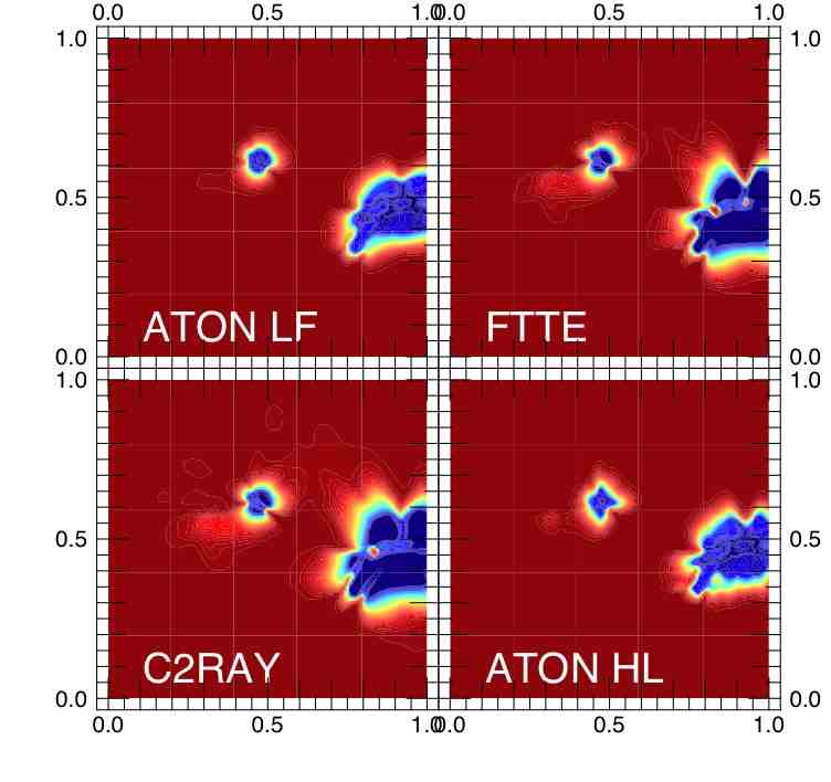
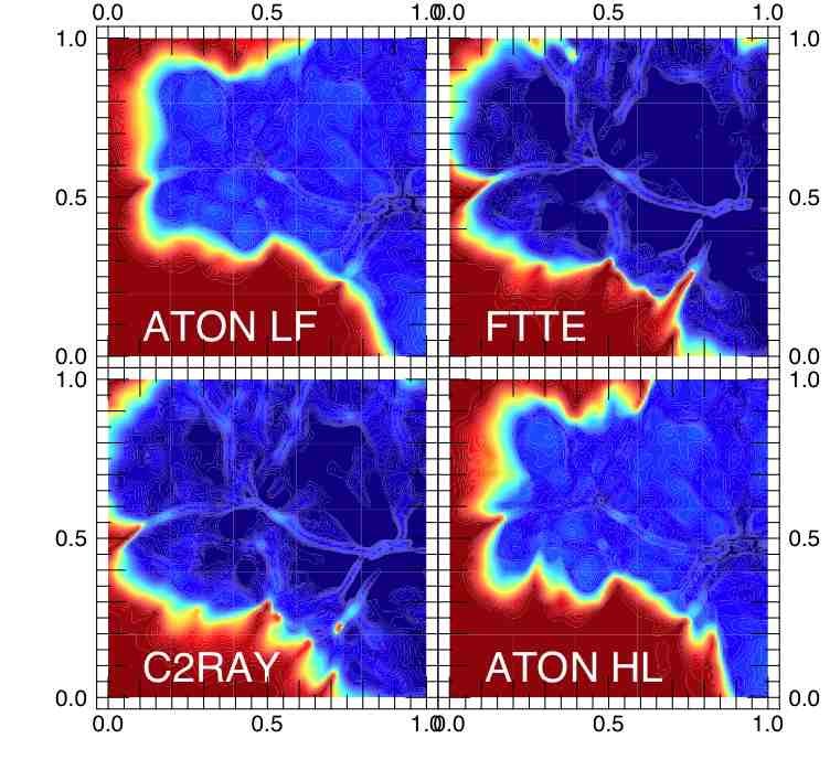
Figure 9: Static cosmological field test. Maps of the neutral fraction computed at 0.05 Myr (Top) and 0.4 Myr (bottom) after the sources were ignited. the four calculations were made using ATON-GLF, ATON-HLL, C2RAY and FTTE.

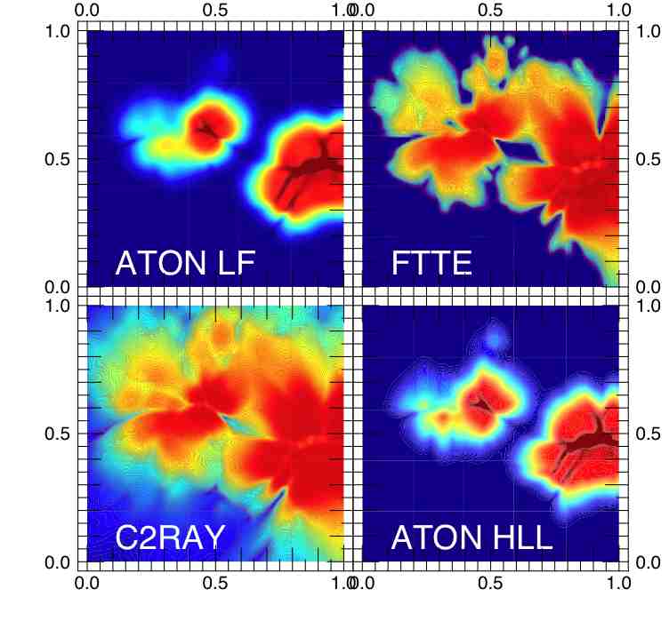
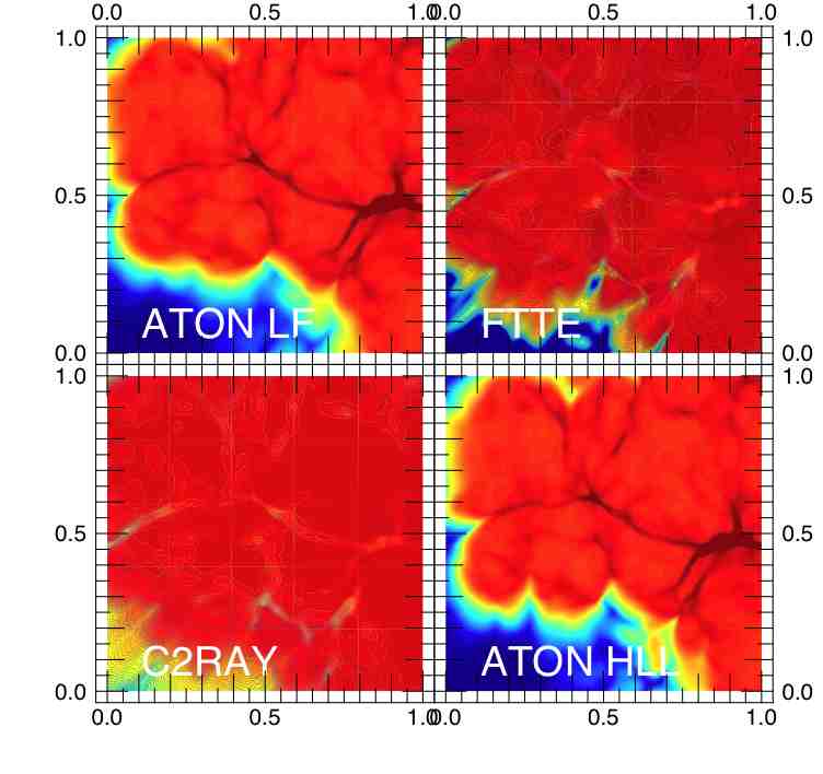
Figure 10: Static cosmological field test. Maps of the temperature computed at 0.05 Myr (Top) and 0.4 Myr (bottom) after the sources were ignited. the four calculations were made using ATON-GLF, ATON-HLL, C2RAY and FTTE.

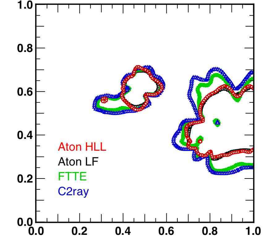
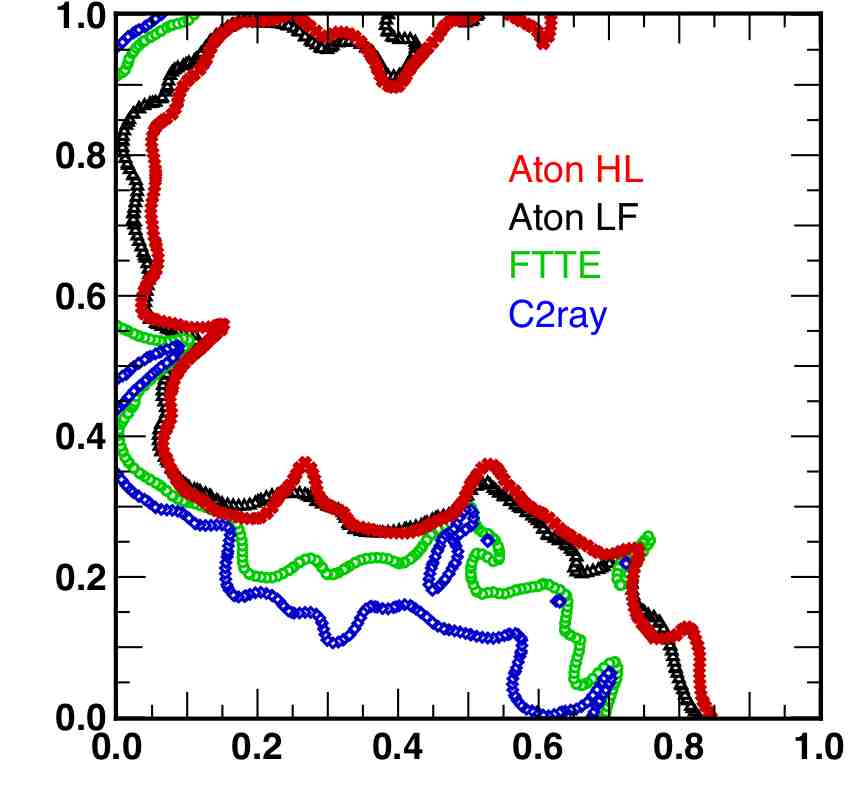
Figure 11: Static cosmological field test. I-front positions (defined as a 50$\%$ ionized fraction) computed at 0.05 Myr (Top) and 0.4 Myr (bottom) after the sources were ignited. the four calculations were made using ATON-GLF, ATON-HLL, C2RAY and FTTE.

Figure 12: Static cosmological field test. Top : the evolution of the average ionized fraction $x_{v}$ (thin lines) and mass-weighted average $x_{m}$ (thick lines). These quantities were computed on snapshots produced by C2RAY, FTTE, ATON-GLF and ATON-HLL. Bottom : the evolution of the ratio $x_{m}/x_{v}$ for the same four calculations.

Figure 13: Static cosmological field test. The evolution of the average ionized fraction $x_{v}$ (thin lines) and mass-weighted average $x_{m}$ (thick lines) using the regular scheme and the “ray–tracing” scheme (with flux mention). An offset of 0.02 has been applied to the latter quantity. GLF (top) and HLL (bottom) intercell flux were used. Clearly the “ray–tracing” scheme do not lead to significant changes in the global evolution of the ionization.

The final test consists in modeling the propagation of I-fronts in an heterogeneous medium with multiple sources. The gas density field consists in a single snapshot extracted from a $128^{3}$ cosmological simulation. The comoving box length is $500h^{-1}$ kpc and for sake of simplicity only the $z=8.9$ snapshot is taken in account and the medium is considered as being static, both from the point of view of cosmology (e.g. no overall expansion) or local motion. A simple source model and distribution was also derived, based on the properties of the biggest haloes. All the sources are turned on a the same time and have $10^{5}$K black-body spectrum. The initial temperature is 100 K and the simulation is ran over 400 000 years, i.e. well before the stationary regime achieved. ATON’s computations are made with an effective speed of light equal to $c$. Further details can be found in Iliev et al. (2006).

Fig. (9) and Fig. (10) present the neutral fraction and the temperature map at t=0.05 Myr and t=0.4 Myr : only the mid-section planes of the simulation are shown. These maps were obtained with the two versions of ATON (GLF and HLL) and compared to the same tests performed by FTTE (Razoumov & Cardall (2005)) and C2RAY (Mellema et al. (2006)) as part of the Iliev et al. (2006) comparison project. Let us emphasize that the simulation is run over 400 000 years only, i.e $0.1\%$ of the recombination time and the regime investigated in this test is highly non-stationary. Clear differences can be noted. First, ATON’s calculations seem to present a delay in the ionization propagation. It can be seen from both maps where ionized and hot regions are typically less extended around the sources in ATON’s calculations compared to the other results. Second, hot regions are more tightly correlated to ionized regions in ATON’s scheme, while FTTE and C2ray show extended and complex structures of hot gas. Since the transition between hot and cooler regions is more abrupt in the ATON’s calculations, it relates to the more compact ionized regions that the current scheme predicts. Furthermore, let us recall that the current implementation of the scheme is ”monochromatic”, even though the average photon’s energy reflects the spectrum of the sources. As a consequence, fronts are sharper and high-energy photons with large travel distances are not available and cannot preheat and preionize the gas on large scales.

Still, given this strong restriction to a single frequency-group treatment, results can be seen as qualitatively satisfying. The I-front positions (see Fig. (11)) with ATON share similar features with the other codes. For instance they coincides along high density regions such as filaments axes. Densities are such that the frequency dependence of cross-section do not penalize the scheme at the current resolution compared to the others and conversely, I-fronts in voids are ”late” in ATON: this supports the fact that the differences are due to the current simplified spectral treatment. This is particularly evident in the $0.05$ Myr map, where a good agreement coincides with filaments and a poor agreement coincides with voids. The $0.4$ Myr maps still hint such correlations but they appear as less obvious since it results from a longer evolution.

The overall ionization evolution is presented in Fig. (12). The average ionized fraction is defined by

$$x_{v}=\frac{\Sigma_{i}^{\mathrm{N}}x_{i}}{\mathrm{N}},$$ (40)

where $N$ stands for the total number of grid cells, $i$ is the cell index and the mass-weighted average ionized fraction by

$$x_{m}=\frac{\Sigma_{i}^{\mathrm{N}}\rho_{i}x_{i}}{\Sigma_{i}^{\mathrm{N}}\rho_{i}},$$ (41)

where $\rho_{i}$ is the local gas density within cell $i$. The ratio of these two quantities is equal to the ratio between the average gas density of ionized regions to the average density (Iliev et al. (2006)) :

$$\frac{x_{m}}{x_{v}}=\frac{M_{\mathrm{ionized}}}{{\bar{\rho}}V_{\mathrm{ionized}}}.$$ (42)

A ratio larger than one implies that ionized regions have densities larger than the average. Conversely a ratio smaller than unity means that voids dominate the ’population’ of ionized regions. Compared to the other codes calculations, ATON exhibits an overall shift of $x_{m}(t)$ and $x_{v}(t)$ in amplitude ($\sim 4\%$ with FTTE and $\sim 12\%$ with C2RAY) while the global trends are similar. One can notice that for all the codes the curves for $x_{m}$ and $x_{v}$ cross each other at some point, implying that high density regions are ionized first while voids tend to be ionized later. The switch operates later in ATON and confirms the code’s slowness in low density regions. Still the discrepancy with other codes remains limited and is encouraging in the prospect of a more complete treatment of multi-frequency transfer. Let us also emphasize that the current set up investigate a highly transient regime and the previous tests have shown that a much better agreement is expected on longer time scales.

Finally, all these tests were performed using also our “ray–tracing” scheme and no significant differences were found (see Fig. (13)). The averaged ionized fractions remain unchanged at the percent level. The maps and the i-front positions (not shown here) are quasi-identical. It implies that even though the isotropic recombination is artificially suppressed, it does not have a strong impact compared to the lack of multi frequency treatment for large scale calculations. In the context of cosmological reionization, future developments would nevertheless focus on these aspects first.

5 Discussion & Conclusion

ATON is a Eulerian scheme for radiative transfer that relies on a momentum description of the radiative transfer equation. The hierarchy set up by the conservation equations of energy and radiative flux is closed by means of a relation between the radiative pressure and the energy. The ’M1’ closure relation has been retained : it expresses the Eddington tensor as the combination of a pure transport configuration of the radiation and a purely diffusive geometry. In the intermediate cases , the relative contribution of these two regimes is obtained from the local flux properties. This scheme is complemented with a a simple treatment of the local chemistry, to compute the neutral hydrogen abundance, and the conservation of energy, to compute the photoheating/cooling. At the current stage, the multi-frequency treatment has not been implemented, even though there are no a priori difficulties for such an extension. ATON is a simple scheme that will eventually be used to investigate astrophysical ionization processes such as the cosmological reionization.

ATON has been tested following the experiments suggested by Iliev et al. (2006): the propagation of an HII region, with and without auto-consistent heating, the shadowing by a dense clump and the I-front propagation in a static cosmological field. Most of the results obtained by ATON are in agreement with the calculations presented in this article. The main differences arises from the lack of multi-frequency treatment : because the spectrum hardening is not taken in account, ionization and heating processes occurs on small scales and for instance no large distance pre-heating due to high energy photons is being modeled at the moment. It results on a loss of radiative energy on small scales and I-fronts tend to be slower in low density regions. However, it only causes problems in highly non stationary regimes while ATON catches all the details of the processes in situations where I-front propagation are slowed down. The issue of the suppression of isotropic recombination was also assessed. For this purpose, we used a modified scheme that mimics ray-tracing codes by taking in account an anisotropic source of flux due to recombination : the results obtained are very similar to ray-tracing or Monte-Carlo codes. However, little differences were observed in the cosmological test, emphasizing the greater impact of the mono-group treatment.

Among the current and future developments, the multi-frequency treatment will follow in order to investigate accurately ionization processes in highly non stationary regimes. Such situations would occur on small scales close to the sources, and these studies would be valuable to constrain e.g. the escape fraction on scales smaller than the resolution of large volume simulations. Also, ATON is limited to the post-processing of simulations and lacks the coupling that exist between the dynamic of the gas and the radiation. Because of its Eulerian nature, the current scheme can be easily coupled with grid based hydrodynamical codes and it is planned to be part of the AMR cosmological code RAMSES (Teyssier, 2002).

Among the astrophysical applications of ATON, the study of the cosmological reinsertion is a primary objective. The post-processing of the AMR and SPH version of a large ongoing hydrodynamical simulation is on the way and will allow to compare the impact of the source distribution and the gas geometry on the reionization process generated by each version . It would also lead to predictions on the geometry of the 21 cm emission, in the prospects of experiments such as SKA or LOFAR. Comparisons on the propagation of radiation in and around the biggest objects, at high resolution are also on the way in order to investigate the impact of small scales clustering of the gas and the star distribution. Hopefully, with the improvements mentioned previously, the current scheme will be able to investigate all the astrophysical processes where radiation is relevant, while remaining simple to conceive and implement.

Acknowledgments

The authors would like to thank E. Audit, I. Iliev and B. Semelin for valuable comments and discussions. A special thanks to M. Gonzalez for providing us his routine to compute the eigenvalues for the M1 Model. We also like to thank the Cosmological Radiative Transfer Comparison Project for making their data publicly available (http://www.cita.utoronto.ca/ iliev/rtwiki/doku.php). This work was performed with support from the HORIZON project (http://www.projet-horizon.fr).

Appendix A Implicit computation of ionization fraction

In ATON, the coupling between radiative energy and ionization fraction is solved implicitly. Let us call $N_{\gamma}$ the density number of photons (i.e. the energy density in single photon units), $F_{\gamma}$ the associated flux, $P_{\gamma}$ the radiative pressure and $x$ the ionization fraction. Let us also define $\rho$ as the initial hydrogen density and $\alpha$, $\alpha_{B}$ and $\beta$ as respectively the case A and case B recombination rates and the collisional ionization rate. First we consider a fixed temperature (from the previous timestep) for the rates computation. The set of coupled (1D) equations is given by

$$\frac{{\mathrm{d}}N_{\gamma}}{{\mathrm{d}}t}+\frac{{\mathrm{d}}F_{\gamma}}{{\mathrm{d}}r} = \dot{N}_{\gamma}^{*}+\dot{N}_{\gamma}^{\mathrm{rec}}-\rho\sigma_{\gamma}cN_{\gamma}(1-x)$$ (43)

$$\frac{{\mathrm{d}}F_{\gamma}}{{\mathrm{d}}t}+\frac{{\mathrm{d}}P_{\gamma}}{{\mathrm{d}}r} = -\rho\sigma_{\gamma}cF_{\gamma}.$$ (44)

Here $\dot{N}_{\gamma}^{*}$ and $\dot{N}_{\gamma}^{\mathrm{rec}}$ stands for the point-like (namely the ’stars’) and the diffuse source of ionizing photons due to recombination and $\sigma_{\gamma}$ stands for the photo-ionization cross-section averaged over the $N_{\gamma}$ spectrum. The ionization equation is given by

$$\frac{{\mathrm{d}}\rho(1-x)}{{\mathrm{d}}t}=\alpha\rho^{2}x^{2}-\beta x(1-x)\rho^{2}-\rho(1-x)N_{\gamma}\sigma_{\gamma}c.$$ (45)

The equation over $n$ can be rewritten as:

$$\frac{{\mathrm{d}}N_{\gamma}}{{\mathrm{d}}t}+\frac{{\mathrm{d}}F_{\gamma}}{{\mathrm{d}}r} = S-\alpha_{B}\rho^{2}x^{2}+\beta x(1-x)\rho^{2}-\rho\frac{{\mathrm{d}}x}{{\mathrm{d}}t},$$ (46)

where we assumed that $\alpha\rho^{2}x^{2}=\dot{N}_{\gamma}^{\mathrm{rec}}+\alpha_{B}\rho^{2}x^{2}$. With $p$ labeling the time step index, we write ${{\mathrm{d}}N_{\gamma}}/{{\mathrm{d}}t}=(N_{\gamma}^{p+1}-N_{\gamma}^{p})/\Delta t$ and $x=x^{p}$ and $X=x^{p+1}$ and the implicit formulation of Eq. (46) is given by:

$$N_{\gamma}^{p+1}=N_{\gamma}{{}^{\prime}}+\beta\rho^{2}(1-X)X\Delta t-\alpha_{B}\rho^{2}X^{2}\Delta t-\rho(X-x),$$ (47)

where $N_{\gamma}^{\prime}$ is the explicit solution of the pure advection equation (i.e. Eq. (43) with a zero r.h.s.) given by:

$$N_{\gamma}^{\prime}=\dot{N}_{\gamma}^{*}\Delta t-\frac{{\mathrm{d}}F_{\gamma}}{{\mathrm{d}}r}\Delta t+N_{\gamma}^{p}.$$ (48)

Combining Eq. (43) and Eq. (47), one can obtain a third-order polynomial $Q_{3}(X)=mX^{3}+nX^{2}+pX+q$, where the coefficients are given by

$$m = (\alpha_{B}+\beta)\rho^{2}\Delta t$$ (49)

$$n = \rho-(\alpha+\beta)\rho/\sigma_{\gamma}c-\alpha_{B}\rho^{2}\Delta t-2\beta\rho^{2}\Delta t$$ (50)

$$p = -\rho(1+x)-N_{\gamma}^{\prime}-1/\sigma_{\gamma}c\Delta t+\beta\rho/\sigma_{\gamma}c+\beta\rho^{2}\Delta t$$ (51)

$$q = N_{\gamma}^{\prime}+\rho x+x/\sigma_{\gamma}c\Delta t,$$ (52)

and where $X$ is given by finding the roots of $Q_{3}(X)$. Knowing $X$, $N_{\gamma}$ is obtained from Eq. (47) and $F_{\gamma}$ can be derived from

$$F_{\gamma}^{p+1}=\frac{F_{\gamma}^{\prime}}{1+c\sigma_{\gamma}\rho\Delta t(1-X)},$$ (53)

where $F_{\gamma}^{\prime}$ is the explicit solution of the the pure advection equation of the flux, given by:

$$F_{\gamma}^{\prime}=F_{\gamma}^{p}-\frac{{\mathrm{d}}P_{\gamma}}{{\mathrm{d}}r}\Delta t.$$ (54)

The temperature at time $t+\Delta t$ is obtained a posteriori, having computed values of $N_{\gamma}^{p+1}$, $F_{\gamma}^{p+1}$ and $x^{p+1}$ while using the temperature set at the previous time step. From Eq. (19), the (discrete) equation that rules the temperature’s evolution is given by:

$$\frac{T^{p+1}-T^{p}}{\Delta t}=\frac{2({\cal H-L}-\frac{3}{2}\rho(1+X)k_{B}T^{p+1}(X-x)/\Delta t)}{3\rho(1+X)k_{B}},$$ (55)

$\cal H$ and $\cal L$ being the heating and cooling rates. Therefore, Eq. (55) can be solved separately in an explicit manner where the R.H.S depends on $T^{p}$ instead of $T^{p+1}$. This equation is purely local and is solved at each cell’s location without any spatial coupling. By simple algebraic manipulation, the updated value of the temperature $T^{p+1}$ can in principle be easily obtained. However, the cooling time becomes much shorter than $\Delta t$ as temperature reach typical value of $\sim 10^{4}$ K, therefore Eq. (55) cannot be solved without resolving this typical time scale.

In practice, Eq. (55) is sub-cycled during a radiative time step, using $\Delta t=0.9t_{\mathrm{c}ool}$. At each ’temperature’ iteration, the cooling rate is updated, setting a new $\Delta t$ for the next iteration. As a consequence such a procedure can substantially increase the computing time. This increase can be reduced by stopping the sub-cycling when some relative convergence of the temperature is achieved. In the tests presented hereafter, a condition such as a $10^{-6}$ convergence after at least $100$ sub-cycles is found to give satisfying result in terms of ionization fraction distributions. Finally the whole process is repeated: the ionized fraction is re-computed using the updated temperature until a global convergence is achieved.

This model is admittedly oversimplified and a full implicit treatment of ionization and photoheating would be preferable. However, it appears from subsequent experiments that taking in account the complexity of the energy-ionization coupling with a temperature that varies in background returns satisfying results. Since temperature is essentially crucial to compute recombination rates, which do not depend strongly on temperature in our case, this simple model appears to be accurate enough at the current stage.

References

- Barkana & Loeb (2001) Barkana R., Loeb A., 2001, Phys. Rep., 349, 125
- Dubroca & Feugeas (1999) Dubroca B., Feugeas J., 1999, C. R. Acad. Sci., 329, 915
- Gnedin & Abel (2001) Gnedin N. Y., Abel T., 2001, New Astronomy, 6, 437
- González et al. (2007) González M., Audit E., Huynh P., 2007, AAP , 464, 429
- Hui & Gnedin (1997) Hui L., Gnedin N. Y., 1997, MNRAS , 292, 27
- Iliev et al. (2006) Iliev I. T., Ciardi B., Alvarez M. A., Maselli A., Ferrara A., Gnedin N. Y., Mellema G., Nakamoto T., Norman M. L., Razoumov A. O., Rijkhorst E.-J., Ritzerveld J., Shapiro P. R., Susa H., Umemura M., Whalen D. J., 2006, MNRAS , 371, 1057
- Iliev et al. (2006) Iliev I. T., Mellema G., Pen U.-L., Merz H., Shapiro P. R., Alvarez M. A., 2006, MNRAS , 369, 1625
- Katz et al. (1996) Katz N., Weinberg D. H., Hernquist L., 1996, ApJS , 105, 19
- Levermore (1984) Levermore C. D., 1984, Journal of Quantitative Spectroscopy and Radiative Transfer, 31, 149
- Madau et al. (1999) Madau P., Haardt F., Rees M. J., 1999, ApJ , 514, 648
- Maselli et al. (2003) Maselli A., Ferrara A., Ciardi B., 2003, MNRAS , 345, 379
- Mellema et al. (2006) Mellema G., Iliev I. T., Alvarez M. A., Shapiro P. R., 2006, New Astronomy, 11, 374
- Mellema et al. (2006) Mellema G., Iliev I. T., Pen U.-L., Shapiro P. R., 2006, MNRAS , 372, 679
- Razoumov & Cardall (2005) Razoumov A. O., Cardall C. Y., 2005, MNRAS , 362, 1413
- Teyssier (2002) Teyssier R., 2002, AAP , 385, 337
- Toro (1999) Toro E., 1999, Riemann Solvers and Numerical Methods for Fluid Dynamics. Berlin, Germany, Springer-Verlag, 1999, 624 p.