Scaling analysis of FLIC fermion actions

Abstract

The Fat Link Irrelevant Clover (FLIC) fermion action is a variant of the $O(a)$-improved Wilson action where the irrelevant operators are constructed using smeared links. While the use of such smearing allows for the use of highly improved definitions of the field strength tensor $F_{\mu\nu},$ we show that the standard 1-loop clover term with a mean field improved coefficient $c_{\rm sw}$ is sufficient to remove the $O(a)$ errors, avoiding the need for non-perturbative tuning. This result enables efficient dynamical simulations in QCD with the FLIC fermion action

I Introduction

The fat-link irrelevant clover (FLIC) fermion action zanotti-hadron is an efficient kamleh-spin Wilson-style nearest-neighbour lattice fermion action which incorporates both the thin gauge-field links of the Markov chain and fat links – links created via APE ape-one ; ape-two ; derek-smooth ; ape-MIT , HYP hyp-smear or stout-link stout-links smearing. Through the use of fat links in the irrelevant operators of the action, one achieves significant improvement in the chiral properties of the action reflected in a narrowing of the distribution of the critical Wilson mass flic-impchiral . One also by-passes the fine-tuning problem typically encountered in ${\cal O}(a)$ improvement, as the use of fat links in both the irrelevant Wilson and clover terms suppresses the otherwise large renormalizations of the improvement coefficients. At the same time, short-distance physics is preserved completely in the action as the relevant operators are constructed with thin links.

Previous work james-scale established the good scaling properties of the Fat Link Irrelevant Clover (FLIC) fermion action when a highly improved definition of the lattice field strength tensor $F_{\mu\nu}$ is used in the clover term. In this work we demonstrate that the use of the standard 1-loop definition of $F_{\mu\nu}$ with fat links in the clover term is sufficient to provide $O(a^{2})$ scaling for FLIC fermions. The 1-loop variant has the advantage of maintaining a simple force term when performing the molecular dynamics portion of a Hybrid Monte Carlo algorithm to generate dynamical configurations.

In Sec. II we highlight the essential features of the FLIC action with a particular emphasis on the various lattice field strength tensors used in the simulations. In addition the $SU(3)$-projection method used to create the fat links is outlined. In Sec. III we describe the methods used to obtain an accurate scale determination on each lattice considered. Simulation parameters and scaling results are presented in Sec. IV while correlation function properties are examined in Sec. V. Conclusions are summarized in Sec. VI.

II FLIC Fermions

The FLIC fermion action zanotti-hadron is a variant of the clover action where the irrelevant operators are constructed using smeared links ape-one ; ape-two , and mean field improvement lepage-mfi is performed. The key point is that short-distance physics is suppressed in the irrelevant operators. This allows an effective mean-field improved calculation of the clover coefficient, required to match the Wilson and clover terms such that $O(a)$ errors are eliminated james-scale . Further, the improved chiral properties of FLIC fermion action allow efficient access to the light quark regime flic-impchiral .

The FLIC operator is given by

$$D_{\rm FLIC}=\nabla\!\!\!\!/\,_{\rm mfi}+\frac{1}{2}(\Delta^{\rm fl}_{\rm mfi}-\frac{1}{2}\sigma\cdot F^{\rm fl}_{\rm mfi})-m\,,$$ (1)

where the presence of fat (or smeared) links and/or mean field improvement has been indicated by the super- and subscripts. The mean field improved lattice gauge covariant derivative is defined by

$$\nabla\!\!\!\!/\,_{\rm mfi}=\sum_{\mu}\frac{1}{2u_{0}}\gamma_{\mu}\left(U_{\mu}(x)\,\delta_{x+\hat{\mu},y}-U_{\mu}^{\dagger}(x-\hat{\mu})\,\delta_{x-\hat{\mu},y}\right),$$ (2)

and likewise the (smeared link) lattice Laplacian is such that

$$\Delta^{\rm fl}_{\rm mfi}=\sum_{\mu}2-\frac{1}{u^{\rm fl}_{0}}\left(U^{\rm fl}_{\mu}(x)\,\delta_{x+\hat{\mu},y}+U_{\mu}^{{\rm fl}\dagger}(x-\hat{\mu})\,\delta_{x-\hat{\mu},y}\right).$$ (3)

We choose $\sigma_{\mu\nu}=\frac{i}{2}[\gamma_{\mu},\gamma_{\nu}].$ For the clover term, one usually selects a standard one-loop $F_{\mu\nu},$

$$F_{\mu\nu}(x) =-\frac{i}{2}(C_{\mu\nu}(x)-C^{\dagger}_{\mu\nu}(x)),$$ (4)

$$C_{\mu\nu}(x) =\frac{1}{4}(U_{\mu,\nu}(x)+U_{-\nu,\mu}(x)$$

$$\qquad+U_{\nu,-\mu}(x)+U_{-\mu,-\nu}(x)),$$ (5)

where $U_{\mu,\nu}(x)=U_{\mu}(x)\,U_{\nu}(x+\hat{\mu})\,U^{\dagger}_{\mu}(x+\hat{\nu})\,U^{\dagger}_{\nu}(x)$ is the elementary plaquette in the $\mu,\nu$ plane. However, with the use of fat links, one is also able to choose highly improved definitions of $F_{\mu\nu}$ sundance-fmunu . Let $C^{m\times n}_{\mu\nu}(x)$ correspond to the sum of the four $m\times n$ loops at the point $x$ in the clover formation, and then define

$$F^{m\times n}_{\mu\nu}(x)=-\frac{i}{2}(C^{m\times n}_{\mu\nu}(x)-C^{\dagger m\times n}_{\mu\nu}(x)).$$ (6)

We can construct a 2-loop field strength tensor which is free of $O(a^{2})$ errors,

$$F^{\rm 2L}_{\mu\nu}=\frac{5}{3}F^{1\times 1}_{\mu\nu}-\frac{1}{6}(F^{1\times 2}_{\mu\nu}+F^{2\times 1}_{\mu\nu}),$$ (7)

or a 3-loop version which is free of $O(a^{4})$ errors,

$$F^{\rm 3L}_{\mu\nu}=\frac{3}{2}F^{1\times 1}_{\mu\nu}-\frac{3}{20}F^{2\times 2}_{\mu\nu}+\frac{1}{90}F^{3\times 3}_{\mu\nu}.$$ (8)

The smeared links in the FLIC action can be equally well constructed from standard APE smeared links, or the more novel stout link method stout-links . As the smeared links only appear in the irrelevant operators, the physics of the action are essentially independent of the choice of smearing method. The only requirement is that sufficient smearing is done such that the mean field improvement becomes an effective means of estimating the clover coefficient $c_{\rm sw}.$ We typically find that four sweeps of APE smearing at $\alpha=0.7$ or four sweeps of stout smearing at $\rho=0.1$ to be sufficient for lattices with a spacing between 0.1 and 0.165 fm.

In this work we use APE smeared links $U^{\rm fl}_{\mu}(x)$ constructed from $U_{\mu}(x)$ by performing $4$ smearing sweeps, where in each sweep we first perform an APE blocking step (at $\alpha=0.7$),

$$V^{(j)}_{\mu}(x)=(1-\alpha)\ \begin{picture}(1.0,1.0)(0.0,0.0) \put(0.0,0.0){\circle*{0.15}} \put(0.0,0.0){\vector(1,0){1.0}} \put(1.0,0.0){\circle{0.14}} \end{picture}+\frac{\alpha}{6}\sum_{\nu\neq\mu}\ \begin{picture}(1.0,1.0)(0.0,0.0) \put(0.0,0.0){\circle*{0.15}} \put(0.0,0.0){\vector(0,1){1.0}} \put(0.0,1.0){\vector(1,0){1.0}} \put(1.0,1.0){\vector(0,-1){1.0}} \put(1.0,0.0){\circle{0.14}} \end{picture}\ +\raisebox{-14.0pt}{ \begin{picture}(1.0,1.0)(0.0,-1.0) \put(0.0,0.0){\circle*{0.15}} \put(0.0,0.0){\vector(0,-1){1.0}} \put(0.0,-1.0){\vector(1,0){1.0}} \put(1.0,-1.0){\vector(0,1){1.0}} \put(1.0,0.0){\circle{0.14}} \end{picture}}\ ,$$ (9)

followed by a projection back into $SU(3),U^{(j)}_{\mu}(x)={\mathcal{P}}(V^{(j)}_{\mu}(x)).$ We follow the “unit-circle” projection method given in kamleh-hmc , which allows for dynamical simulations. The projection is defined by first performing a projection into $U(3)$

$$U^{\prime}(V)=V[V^{\dagger}V]^{-\frac{1}{2}},$$ (10)

followed by projection into $SU(3)$

$${\mathcal{P}}(V)=\frac{1}{\sqrt[3]{\det U^{\prime}(V)}}\,U^{\prime}(V)\,.$$ (11)

It should be noted that the principal value of the cube root (being that with the largest real part) is the appropriate branch of the cube root function to choose. As noted in kamleh-hmc this choice provides the mean link which is closest to unity.

Mean field improvement is performed by making the replacements

$$U_{\mu}(x)\to\frac{U_{\mu}(x)}{u_{0}},\quad U^{\rm fl}_{\mu}(x)\to\frac{U^{\rm fl}_{\mu}(x)}{u^{\rm fl}_{0}},$$ (12)

where $u_{0}$ and $u_{0}^{\rm fl}$ are the mean links for the standard and fattened links. We calculate the mean link via the fourth root of the average plaquette

$$u_{0}=\left\langle{\rm\frac{1}{3}\,Re\,Tr}\,U_{\mu\nu}(x)\right\rangle_{x,\,\mu<\nu}^{\frac{1}{4}}\,.$$ (13)

III Scale determination

The scale is determined using a 4-parameter ansatz

$$V({\rm\bf r})=V_{0}+\sigma\,r-e\left[\frac{1}{\rm\bf r}\right]+l\left(\left[\frac{1}{\rm\bf r}\right]-\frac{1}{r}\right)$$ (14)

as in Ref. accurate-scale . The tree-level lattice Coulomb term used in the ansatz is given by

$$\left[\frac{1}{\rm\bf r}\right]=4\pi\int\frac{d^{3}{\rm\bf k}}{2\pi^{3}}\,\cos({\rm\bf k\cdot r})\,D_{00}(0,{\rm\bf k}).$$ (15)

Here $D_{00}(0,{\rm\bf k})$ comes from the tree-level gluon propagator for the appropriate gluon action. For the Wilson gluon action, we have at tree-level,

$$D^{-1}_{00}(0,{\rm\bf k})=4\sum_{\mu=1}^{3}\sin^{2}\frac{k_{\mu}}{2},$$ (16)

where on a lattice with extents $L_{\mu}$ the allowed momenta are

$$k_{\mu}=\frac{2\pi n_{\mu}}{L_{\mu}},\quad-\frac{L_{\mu}}{2}<n_{\mu}\leq\frac{L_{\mu}}{2}\,.$$ (17)

For the Lüscher-Weisz gluon action, we have at tree-level,

$$D^{-1}_{00}(0,{\rm\bf k})=4\sum_{\mu}\left(\sin^{2}\frac{k_{\mu}}{2}+\frac{1}{3}\sin^{4}\frac{k_{\mu}}{2}\right).$$ (18)

The lattice Coulomb term is constructed by calculating on large lattice volumes and then extrapolating to infinite volume. Explicitly, we choose $L=128$ and $L=256$ and calculate $\left[\frac{1}{\rm\bf r}\right]_{L}$ for an $L^{3}$ spatial volume. On a finite volume, the Coulomb term takes the form urs-private

$$\frac{1}{r}+\frac{1}{L-r}=\frac{1}{r}+\frac{1}{L}+O\left(\frac{r}{L^{2}}\right).$$ (19)

In order to calculate the infinite volume tree-level lattice Coulomb term $\left[\frac{1}{\rm\bf r}\right]$, we extrapolate $\left[\frac{1}{\rm\bf r}\right]_{L}$ linearly in $\frac{1}{L}$ to $\frac{1}{L}=0$.

The tree-level lattice Coulomb term $\left[\frac{1}{\rm\bf r}\right]$ for the Wilson and Lüscher-Weisz gauge action is shown in Fig 1. The important finite lattice spacing artefacts are revealed at small $r\lesssim 3\,a$. The ${\cal O}(a^{2})$ improvement in the Lüscher-Weisz Coulomb term is also readily apparent.

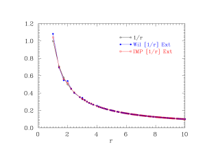
Figure 1: The (infinite volume) tree-level lattice Coulomb term for the Wilson and Lüscher-Weisz (IMP) gauge action.

Figure 2: The scaling of the $N$ and $\rho$ masses for various quark actions in the quenched approximation according to the string tension (upper) and the Sommer scale (lower).

IV Scaling Results

Calculations are performed on mean-field improved plaquette plus rectangle $SU(3)$ Lüscher-Weisz lattices. Lattice spacings determined using fits to Eq. (14) above are given in Table 1.

$\beta$	$a[\sigma]{\rm(fm)}$	$a[r_{0}]{\rm(fm)}$
4.80	0.096(1)	0.088(1)
4.60	0.120(1)	0.113(1)
4.53	0.132(1)	0.124(1)
4.38	0.164(1)	0.152(1)

Table 1: The lattice spacing for pure Lüscher-Weisz glue determined by the string tension $\sqrt{\sigma}=440\text{ MeV}$ and the Sommer scale $r_{0}=0.49\text{ fm}$ for various couplings $\beta$.

	$\beta$	$M_{N}/\sqrt{\sigma}$	$M_{\rho}/\sqrt{\sigma}$	$M_{N}r_{0}$	$M_{\rho}r_{0}$
FLIC-1L	4.60	2.278(26)	3.347(33)	2.638(30)	3.875(39)
	4.53	2.313(27)	3.368(41)	2.662(31)	3.876(47)
	4.38	2.299(21)	3.323(32)	2.688(25)	3.886(38)
FLIC-2L	4.60	2.347(26)	3.394(33)	2.717(30)	3.929(39)
	4.53	2.39(30)	3.453(44)	2.751(35)	3.974(51)
	4.38	2.41(24)	3.450(35)	2.818(28)	4.034(41)
FLIC-3L	4.60	2.365(30)	3.461(37)	2.738(34)	4.006(43)
	4.53	2.413(37)	3.478(48)	2.776(43)	4.003(55)
	4.38	2.435(27)	3.474(38)	2.847(32)	4.062(44)

Table 2: Results for the $N$ and $\rho$ masses on the three lattices, for the scale determined by the string tension $\sigma$ and the Sommer scale $r_{0}$.

Figure 3: $\rho-$meson correlation functions at two approximately matched quark masses for the 1-loop (top), 2-loop (middle) and 3-loop (bottom) FLIC actions. Two lattices at $16^{3}\times 32$ are shown, $\beta=4.60$ (left) and $\beta=4.53$ (right).

For each of the lattices we calculate quark propagators using the FLIC fermion action with a 1, 2 and 3-loop clover term as described in Sec. II. The $\pi,\rho$ and $N$ masses are then calculated and interpolated to a $\pi/\rho$ mass ratio of 0.7, shown in Table 2.

Scaling results are presented in Fig. 2. The lines of fit are extrapolations in $a^{2}$ constrained to pass through the single point at the continuum limit. The lines for non-perturbatively improved clover and all FLIC actions are straight, indicating $O(a^{2})$ scaling, that is the effective elimination of $O(a)$ errors.

Thus, 1-, 2- and 3-loop fat-link formulations of $F_{\mu\nu}$ in the FLIC fermion action all provide $O(a)$ improvement as expected. The different formulations differ at the level of $O(a^{2}).$ Remarkably, the 1-loop action is actually the preferred action. Firstly, it is the cheapest to perform molecular dynamics with, which is important for Hybrid Monte Carlo dynamical simulations. Secondly it has the smallest residual $O(a^{2})$ errors in the quantities we have studied here. We’ll also see that correlation functions have smaller fluctuations.

V Correlation Functions

Finally, we compare the $\rho-$meson correlation function on the fine $\beta=4.60$ and coarse $\beta=4.53$ lattices at approximately matched pion masses for the three different FLIC actions. The source is at time slice 8.

The effective mass plots are given in Figure 3. The main effect that we observe is that as the Euclidean time index progresses into the latter half of the lattice, the 1-loop FLIC correlators show reduced fluctuations and reduced error bars when compared with the 2-loop and 3-loop FLIC results. The difference is particularly observable on the coarser $\beta=4.53$ lattice. We understand this to be due to the 1-loop action having a more local field strength $F_{\mu\nu}(x)$ than the 2- and 3-loop actions making it less susceptible to large fluctuations.

VI Conclusions

We have examined the role of improvement in the lattice field strength tensor of the FLIC fermion action, Our results demonstrate that the standard 1-loop choice of for the lattice clover term in the FLIC fermion action provides $O(a^{2})$ scaling.

Remarkably the 1-loop action provides results that are preferable to those obtained from the 2-loop ${\cal O}(a^{2})$-improved lattice field strength tensor or those obtained from the the 3-loop ${\cal O}(a^{4})$-improved definition. The 1-loop results provide

1. Smaller residual $O(a^{2})$ errors,

2. Stable hadron correlators with reduced fluctuations,

3. Smaller statistical uncertainties, and

4. A more efficient action suitable for dynamical fermion simulations.

This result enables efficient and effective dynamical QCD simulations with FLIC fermions. Simulations are currently under way.

References

- (1) CSSM Lattice, J. M. Zanotti et al., Phys. Rev. D65, 074507 (2002), hep-lat/0110216.
- (2) W. Kamleh, (2002), hep-lat/0209154.
- (3) M. Falcioni, M. L. Paciello, G. Parisi, and B. Taglienti, Nucl. Phys. B251, 624 (1985).
- (4) APE, M. Albanese et al., Phys. Lett. B192, 163 (1987).
- (5) F. D. R. Bonnet, D. B. Leinweber, A. G. Williams, and J. M. Zanotti, (2001), hep-lat/0106023.
- (6) M. C. Chu, J. M. Grandy, S. Huang, and J. W. Negele, Phys. Rev. D49, 6039 (1994), hep-lat/9312071.
- (7) A. Hasenfratz and F. Knechtli, Phys. Rev. D 64, 034504 (2001), hep-lat/0103029.
- (8) C. Morningstar and M. Peardon, (2003), hep-lat/0311018.
- (9) S. Boinepalli, W. Kamleh, D. B. Leinweber, A. G. Williams, and J. M. Zanotti, Phys. Lett. B616, 196 (2005), hep-lat/0405026.
- (10) J. M. Zanotti, B. Lasscock, D. B. Leinweber, and A. G. Williams, Phys. Rev. D71, 034510 (2005), hep-lat/0405015.
- (11) G. P. Lepage and P. B. Mackenzie, Phys. Rev. D48, 2250 (1993), hep-lat/9209022.
- (12) S. O. Bilson-Thompson, D. B. Leinweber, and A. G. Williams, Ann. Phys. 304, 1 (2003), hep-lat/0203008.
- (13) W. Kamleh, D. B. Leinweber, and A. G. Williams, Phys. Rev. D70, 014502 (2004), hep-lat/0403019.
- (14) R. G. Edwards, U. M. Heller, and T. R. Klassen, Nucl. Phys. B517, 377 (1998), hep-lat/9711003.
- (15) U. Heller, Private communication .