On the efficiency of field star capture by star clusters

Abstract

Context. An exciting recent finding regarding scaling relations among globular clusters is the so-called ’blue tilt’: clusters of the blue sub-population follow a trend of redder colour with increasing luminosity.

Aims. In this paper we evaluate to which extent field star capture over a Hubble time changes the photometric properties of star clusters. Given that field stars in early type giant galaxies are very metal-rich, their capture will make blue GCs redder and may in principle explain the ’blue tilt’.

Methods. We perform collisional N-body simulations to quantify the amount of field star capture occuring over a Hubble time to star clusters with 10³ to 10⁶ stars. In the simulations we follow the orbits of field stars passing through a star cluster and calculate the energy change that the field stars experience due to gravitational interaction with cluster stars during one passage through the cluster. The capture condition is that their total energy after the passage is smaller than the gravitational potential at the cluster’s tidal radius. By folding this with the fly-by rates of field stars with an assumed space density as in the solar neighbourhood and a range of velocity dispersions $\sigma$ (15 to 485 km$s^{-1}$), we derive estimates on the mass fraction of captured field stars as a function of environment.

Results. We find that integrated over a Hubble time, the ratio between captured field stars and total number of clusters stars is very low ($\lesssim 10^{-4}$), even for the smallest field star velocity dispersion $\sigma=$15 km$s^{-1}$. This holds for star clusters in the mass range of both open clusters and globular clusters. We furthermore show that tidal friction has a negligible effect on the energy distribution of field stars after interaction with the cluster. We note that field star capture at the time of cluster formation, when the cluster potential increases with time, is more efficient. However, it cannot explain the trend that more massive star clusters are redder.

Conclusions. Field star capture is not a probable mechanism for creating the colour-magnitude trend of metal-poor globular clusters.

1 Introduction

An exciting recent finding regarding scaling relations among globular clusters is that the colours of individual globular clusters (GCs) of the blue sub-population are correlated with their luminosities. This correlation is such that brighter globulars are redder (Harris et al. Harris06 (2006), Mieske et al. Mieske06 (2006), Strader et al. Strade06 (2006), Spitler et al. Spitle06 (2006), Cantiello et al. Cantie07 (2007)). The amplitude of this ’blue tilt’ is about 0.03 to 0.04 mag in colour per mag in luminosity. Assuming coeval GCs, the trend implies a relation between mass of the GCs and the luminosity weighted mean metallicity of its member stars. Various mechanisms have been discussed that may offer ways towards explain the trend, like self-enrichment (Strader et al. Spitle06 (2006)) or “sample contamination” by stripped nuclei of dwarf galaxies (Harris et al. Harris06 (2006), Bekki et al. Bekki07 (2007)).

Self-enrichment, especially if pressure-induced (Mieske et al. Mieske06 (2006), Parmentier Parmen04 (2004)), may offer a plausible way toward explaining the trend. Numerous authors have discussed the possibility of star cluster self enrichment, but there is a wide range of conclusions as to whether and to which extent it is possible in GCs (e.g., Frank & Gisler Frank76 (1976), Smith Smith96 (1996), Gnedin et al.  Gnedin02 (2002), Parmentier & Gilmore Parmen01 (2001), Dopita & Smith Dopita86 (1986), Morgan & Lake Morgan89 (1989), Thoul et al.  Thoul02 (2002), Recchi & Danziger Recchi05 (2005), Prantzos & Charbonnel Prantz06 (2006)).

The presence of contaminators like stripped nuclei can probably not give a satisfactory explanation for the trend. Given the Gaussian shape of the blue colour peak (Bekki et al. Bekki07 (2007), Peng et al. Peng06 (2006)) over the observed magnitude range, one would require the “contaminators” to actually dominate the GC sample. This is unlikely, given the much smaller number of stripped nuclei expected over a Hubble time (Bekki et al. Bekki03 (2003), Mieske et al. Mieske06 (2006)).

In Mieske et al. (Mieske06 (2006), M06 in the following) we indicate that also the capture of field stars in giant elliptical galaxies can in principle cause such colour-magnitude trends, including the dependence of the trend on field star density that is detected in M06. This is because the field star population is generally much redder than the blue globular clusters. Assuming a non-linear dependence of the capture efficiency on globular cluster mass, a colour-mass trend will occur. The question is whether clusters can obtain a sufficiently large population of captured field stars (several percent) to create a notable trend. More generally, it is also of interest to which extent field star capture may explain the multiple populations detected in massive Milky Way globular clusters (e.g. Bedin et al. Bedin04 (2004), D’Antona et al. Danton05 (2005), Piotto et al. Piotto07 (2007)).

In this paper, we present collisional N-body simulations to quantify the amount of field star capture occuring over a Hubble time to star clusters with a time-invariant gravitational potential. The setup of the simulations is presented in Sect. 2, the results are shown in Sect. 3. The discussion in Sect. 4 includes a comparison between our results and estimates on field star capture in bulge globular clusters from Bica et al. (Bica97 (1997)), which are markedly different.

2 Setup of simulations

We simulate the passage of field stars through a star cluster by means of direct $N$-body simulations, using a fourth order Hermite scheme with individual time-steps to follow the orbits of field and cluster stars. For the sake of simplicity we do not include the tidal field of the host galaxy in the calculations. This is justified since interactions are restricted to the central, high density parts of the cluster, where the host galaxy potential does not play a role. The host galaxy properties are folded in later, when capture probabilities are derived as a function of the ratio between tidal radius r_tid and cluster half-mass radius r_h. We assume a time-invariant gravitational potential for the star clusters, since the typical crossing times of a few Myr are very small compared to mass loss time scales (e.g. Baumgardt & Makino BM03 (2003), Lamers et al. Lamers05 (2006)). In our calculations, the interactions between field stars and cluster stars are calculated at each time step, while the cluster stars do not interact among themselves, but rather feel a smooth cluster potential. Allowing for direct interactions between the cluster stars would have increased the required computation time to prohibitively large values. We have therefore not included this case in the present study. It is in any case unlikely that direct interactions between cluster stars influence our results: the interaction of the field stars with the cluster stars happens on a crossing time, while interactions between cluster stars lead to orbital changes only on a relaxation time, which is at least a factor of 100 longer for the considered clusters.

We simulate three star clusters with particle numbers of N=$10^{3}$, $10^{4}$, and 10⁵, assuming a Plummer profile for the stellar density distribution. Three different values of the initial radial velocity at infinity of the field stars v_ini are simulated, namely v_ini=0.1, 0.33, and 1 $\sigma_{\rm cluster}$, where $\sigma_{\rm cluster}$ is the velocity dispersion of the star cluster. For each particle number and field star velocity, we simulate the passage of 10⁴ field stars.

The distance of closest approach $p(b)$ as a function of the initial impact parameter $b$ at infinity is given by

$$p(b)=-G*M_{c}/v_{\rm ini}^{2}+\sqrt{(G*M_{c}/v_{\rm ini}^{2})^{2}+b^{2}}$$ (1)

where $M_{c}$ is the mass of the cluster and $G$ the gravitational constant. For the direct numerical calculation of a given field star’s trajectory, we restrict the distance of closest passage $p(b)$ to smaller than two half-mass radii of the star cluster since larger impact parameters do not result in any notable interaction between cluster and field stars and can hence be excluded from our runs (see Fig. 1). The initial impact parameter $b$ of each star is chosen randomly within the surface area that corresponds to $p<2*r_{\rm h}$. The direct numerical calculation for a given field star is started at a distance of 2 $r_{\rm tid}$. The velocity and position at this distance are calculated by analytically integrating the orbit, assuming a Keplerian ellipse with parameters based on $b$ and v_ini. After following each individual passage, a star is considered as captured if its total energy $E$ after the interaction is smaller than the potential energy at the tidal radius: $E<\frac{-GM_{c}}{r_{\rm tid}}$.

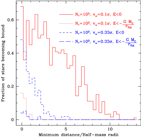
Figure 1: The fraction of captured field stars vs. the minimum distance to the cluster centre for different initial stellar velocities and capture criteria. For the dotted and long-dashed curves, a tidal radius of $r_{tid}=20r_{h}$ was assumed, while the solid and short-dashed curves assume no tidal field of the galaxy. For star clusters in tidal fields, significant capture of field stars occurs only for impact parameters $p$ smaller than 2$r_{h}$.

3 Results

3.1 Capture probabilities

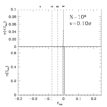
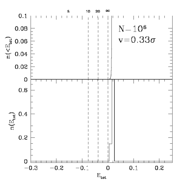
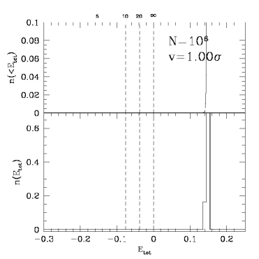
Figure 3: Energy distributions of field stars after interaction like in Fig. 2, but here for clusters with $N$=10⁵ (left) and 10⁶ (right) stars. The curves for $N$=10⁶ result from re-scaling the distribution of $N$=10⁵ (see text). For high particle numbers, only a very small fraction of incoming field stars gets bound to the clusters.

Figs. 2 and 3 show the energy distribution of field stars after interaction with the cluster stars. The results for clusters with $N$=10³ to 10⁵ stars are directly taken from the corresponding N-body simulations. In Fig. 3 we also plot results for $N=10^{6}$, where we have re-scaled the results from lower $N$ (see below). This was done since calculations for large numbers of cluster stars require exceedingly large calculation times.

In the units of the calculations shown in Figs. 2 and 3, the mean kinetic energy of the cluster stars is 0.14582, which is equal to the total initial energy of field stars when $v_{ini}=\sigma_{\rm cluster}$.

Due to the encounters between cluster and field stars, the energy distribution of the field stars gets broadened. If relaxation is responsible for the broadening, one would expect that the dispersion in energy of the field stars after the passage should be proportional to

$$\frac{\Delta E}{E}\sim\sqrt{\frac{t_{\rm Pass}}{t_{\rm rel}}}$$ (2)

where $t_{\rm Pass}$ is the crossing time of the field stars through the cluster and $t_{\rm rel}$ is the clusters relaxation time. Since $t_{\rm rel}\sim\frac{N}{\ln{N}}$, the energy distribution should become narrower for a larger number of cluster stars, which is indeed observed in the runs. For v_ini=0.1$\sigma_{\rm cluster}$, the width for $N$=10⁴ is a factor of $\sqrt{9.4}$ smaller than for $N$=10³, and a factor of $\sqrt{9.1}$ larger than for $N$=10⁵. The corresponding factors for a scaling with the relaxation time are $\sqrt{7.5}$ and $\sqrt{8.0}$, which is close to the observed scaling. The reason for the remaining difference could be close enocunters between cluster and field stars, which lead to large energy changes and are not correctly described by relaxation. Since close encounters are more important for low-mass clusters, the difference with the observed scaling should become smaller for larger $N$, which is indeed the case.

On the other hand, the width depends only very marginally on the initial velocity: the width for v_ini=0.1$\sigma_{\rm cluster}$ and $N$=10⁴ is only 17% broader than for v_ini=1.0$\sigma_{\rm cluster}$ for $N$=10⁴. Energy conservation requires the velocity of a field star near the half-mass radius to be given by $v_{*}=\sqrt{2\sigma_{\rm cluster}^{2}+v^{2}_{\rm ini}}$. Since the crossing time is inversely proportional to $v_{*}$, we would expect that the width is 22% higher for v_ini=0.1$\sigma_{\rm cluster}$, which is close to the above value. Those well defined dependencies allow us to make a robust extrapolation of the capture probabilities from $N$=10⁵ to $N$=10⁶ to estimate capture rates of massive globular clusters.

To obtain estimates for $N$=10⁶ we re-scaled the energy distributions for 10⁵ by reducing its width by a factor of $\sqrt{8.3}$. This is the reduction factor expected from $t_{\rm rel}\sim\frac{N}{\ln{N}}$. From the comparisons above we would expect this reduction factor to be a lower limit. Thus, the number of field stars below a certain energy that are derived from this re-scaling will be a slight over-estimate of the true number. The mean of the energy distributions for the various v_ini was adopted identical to the values for $N$=10⁵. This is possible because the mean total energy of stars after interaction is identical to the initial energy. The implicit assumption that tidal friction is negligible is discussed in Sect. 4. In order to achieve a statistical precision of the extrapolation to better than 10^-4 (i.e. the inverse of the number of simulated stars), we fitted $t$-functions to the energy distributions of the $N$=10⁵ cluster and re-scaled this continuous function to estimate the capture probability for a $N$=10⁶ cluster. For the fitting, we took special care to not underestimate the wings of the energy distribution. See Fig. 4 for a comparison between the continuous fit and the discrete energy distribution of field stars for the $N$=10⁵ cluster and v${}_{\rm ini}=0.1\sigma_{\rm cluster}$.

In each plot of Figs. 2 and 3 we indicate the potential energy at $r_{\rm tid}=$5, 10, and 20$\times r_{h}$. These values are typical tidal radii for open or globular clusters that have a half-mass radius of a few pc and move on orbits which are a few kpc away from the center of a Milky Way like galaxy. The upper part of each plot shows the cumulative energy distribution of the field stars after the interaction. The fraction of captured field stars for a given $r_{\rm tid}$ is determined by the intersection of the cumulative distribution and the corresponding vertical dashed line. The numerical values for $r_{\rm tid}$=5, 10 and 20 $\times r_{h}$ are given in Table 1. As can be seen, the capture probability is extremely low especially for large initial velocities $\sim\sigma_{\rm cluster}$. However, even for small initial relative velocities and large assumed tidal radii the probabilities are negligible for most cases. Only for the very low mass case ($N$=10³) of a small open cluster, the capture probabilites are a few percent for field stars with initial velocities smaller than $\sigma_{\rm cluster}$.

Table 1: Field star capture probabilities as function of field star initial velocity and number of cluster stars $N$. Probabilities refer to field stars with impact parameter $p<2r_{h}$. For $N$=10³ to 10⁵, the numbers are directly taken from N-body simulations of 10000 field star passages. For $N$=10⁶, the probabilities are taken from a fit to the energy distribution of $N$=10⁵ which was re-scaled to the expected width for $N$=10⁶ (see text and Fig. 4).

$N$	$r_{\rm tid}$	vini=0.1$\sigma_{\rm cluster}$	vini=0.33$\sigma_{\rm cluster}$	vini=1.0$\sigma_{\rm cluster}$
103	$5\times r_{\rm h}$	4.7*10-3	2.2*10-3	7*10-4
103	$10\times r_{\rm h}$	2.33*10-2	1.28*10-2	1.3*10-3
103	$20\times r_{\rm h}$	8.49*10-2	4.55*10-2	1.7*10-3
104	$5\times r_{\rm h}$	4*10-4	2*10-4	2*10-4
104	$10\times r_{\rm h}$	1.1*10-3	5*10-4	2*10-4
104	$20\times r_{\rm h}$	6.7*10-3	2.4*10-3	2*10-4
105	$5\times r_{\rm h}$	$<5*10^{-5}$	$1*10^{-4}$	$<5*10^{-5}$
105	$10\times r_{\rm h}$	$<5*10^{-5}$	$3*10^{-4}$	$<5*10^{-5}$
105	$20\times r_{\rm h}$	1*$10^{-4}$	$3*10^{-4}$	$<5*10^{-5}$
106	$5\times r_{\rm h}$	$3*10^{-7}$	$3*10^{-7}$	$<10^{-7}$
106	$10\times r_{\rm h}$	$1.9*10^{-6}$	$1.4*10^{-6}$	$<10^{-7}$
106	$20\times r_{\rm h}$	$1.2*10^{-5}$	$5*10^{-6}$	$1*10^{-7}$

3.2 Capture rates

To transform the capture probabilities into actual capture rates, we need to know the number of ’fly-by’ field stars. These are those stars that over 10 Gyr approach the cluster within 2*$r_{\rm h}$ and within the various $v_{\rm ini}$ ranges. It is important to re-iterate that the initial velocities $v_{\rm ini}$ in Table 1 are expressed in units of star cluster velocity dispersion $\sigma_{\rm cluster}$. Depending on which mass is assumed for a single star, these ranges correspond to different ranges in km/s. In the following we adopt as mass of a single star 0.5 solar masses, which is the typical average mass of stars in clusters of the investigated range. The mass range of the investigated cases hence ranges from 0.5 * 10³ to 0.5 * 10⁶ M_☉. This covers the regime from open clusters up to globular clusters one magnitude more massive than the mass-function turn-over (2*10⁵ M_☉, e.g. Jordán et al. Jordan07 (2007)).

For calculating the fly-by rates, we assume a typical globular cluster half-mass radius of $r_{h}=3$ pc (Jordán et al. Jordan05 (2005) and Jordan07 (2007)). Furthermore, we adopt a field star density of 0.1 $L_{\sun}pc^{-3}$, which is comparable to typical values in giant elliptical galaxies within $r_{\rm eff}$ (Romanowsky et al. Romano01 (2001)), and also similar to the value in the solar neighbourhood. Assuming a typical M/L ratio of 2.5, this corresponds to a mass density of 0.25 $M_{\sun}pc^{-3}$.

The resulting fly-by rates are shown in Table 2. The calculations are done for masses between 0.5*10³ and 0.5*10⁶ $M_{\sun}$, and for a range of relative velocity dispersions between field stars and cluster. The highest velocity dispersion (485 km/s) represents the case of a GC orbiting a giant elliptical galaxy like M87 (see Mieske et al. Mieske06 (2006)). The lowest velocity dispersion (15 km/s) represents co-rotation of an open or globular cluster in a dynamically cold disk. The number of fly-by stars is given as fraction of the number of stars in the cluster. For high field star velocity dispersions and low cluster masses, not a single field star with $v<\sigma_{\rm cluster}$ passes the cluster over a Hubble time.

The capture probabilities (assuming 0.5 solar mass stars) convolved with the number of “fly-bys” within 10 Gyrs yields the mass fraction of captured field stars. These numbers are shown in Table 3 for the case of $r_{\rm tid}=$20$\times r_{h}$. For most cases, the number of captured field stars is lower than 1 single star over a Hubble time. Only for the more massive examples 0.5*10⁴ to 0.5*10⁶ $M_{\sun}$ and the cold disk case, up to a few dozen stars will be captured. The mass fraction of captured stars is $\leq 2*10^{-4}$ for all considered cases.

This shows that field star capture over a Hubble-time will not change the integrated photometric parameters of a star cluster.

Figure 2: Distribution of total energy E_tot of field stars after interaction with the cluster stars. Left panels: Star clusters with $N$=10³ stars. Right panels: Star clusters with $N$=10⁴ stars. Bottom panels give the energy histogram, top panels give the cumulative stellar distribution. Indicated in each plot are the number of cluster stars and the field star initial velocities in units of the star cluster velocity dispersion $\sigma_{\rm cluster}$. The initial energies corresponding to the three cases of v=1.0, 0.33 and 0.1 $\sigma$ are (in model units): 0.146, 0.0159, and 0.00146. They coincide with the peaks of the respective energy distributions. The requirement for field star capture is $E_{tot}<\frac{-GM_{c}}{r_{\rm tid}}$, with $r_{\rm tid}$ being the tidal radius of the cluster in the gravitational field of the host galaxy. The vertical dashed lines indicate different assumed ratios of $\frac{r_{\rm tid}}{r_{h}}$, where $r_{h}$ is the cluster’s half-mass radius.

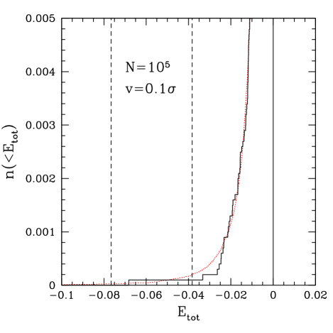
Figure 4: Cumulative distribution of total energy E_tot of field stars after interaction with the cluster stars for $M_{c}=0.5*10^{5}$M_∗ and v=$0.1\sigma_{\rm cluster}$. Solid (black) histogram shows the result of N-body simulations. The dotted line is the cumulative version of a $t$-distribution chosen to fit the simulated distribution. This continuous function is used to extrapolate the capture probabilities for $N$=10⁶ clusters (see text and Table 1). The two vertical dashed lines indicate the energy required for capture for two different ratios between the cluster’s tidal and half-mass radii. For the more negative energy, it is $\frac{r_{\rm tid}}{r_{h}}=10$. For the less negative energy, it is $\frac{r_{\rm tid}}{r_{h}}=20$.

Table 2: Fraction of field stars over cluster stars f($\sigma_{\rm field}$) that approach a star cluster within 10 Gyr and within 2*$r_{\rm h}$, within adjacent ranges around $v_{\rm ini}$ indicated in column 3. $\frac{v_{\rm ini}}{\sigma_{\rm cluster}}=0.1$ corresponds to the range [0 : 0.18]. $\frac{v_{\rm ini}}{\sigma_{\rm cluster}}=0.33$ corresponds to [0.18 : 0.57]. $\frac{v_{\rm ini}}{\sigma_{\rm cluster}}=1$ corresponds to [0.57 : 1]. The star cluster is assumed to have $r_{\rm h}=3pc$, consist of 0.5 solar mass stars, and be embedded within a field star density of 0.1 $L_{\sun}pc^{-3}$. The approach fractions (or “fly-by” rates) are calculated for different assumed velocity dispersions of the field stars $\sigma_{\rm field}$.

Mass [M☉]	$\sigma_{\rm cluster}$ [km/s]	$\frac{v_{\rm ini}}{\sigma_{\rm cluster}}$	f($\sigma_{\rm field}=485$ km s-1)	f($\sigma_{\rm field}=200$ km s-1)	f($\sigma_{\rm field}=50$ km s-1)	f($\sigma_{\rm field}=15$ km s-1)
0.5*103	0.4	0.1	0	0	0	1*10-3
0.5*103	0.4	0.33	0	0	0	5*10-3
0.5*103	0.4	1	0	0	0	1.2*10-2
0.5*104	1.3	0.1	0	0	1.5*10-4	5*10-3
0.5*104	1.3	0.33	0	0	1.4*10-3	5*10-2
0.5*104	1.3	1	0	0	3.6*10-3	0.13
0.5*105	4.2	0.1	0	2*10-5	1.5*10-3	6*10-2
0.5*105	4.2	0.33	1.6*10-5	2*10-4	1.4*10-2	0.52
0.5*105	4.2	1	4*10-5	6*10-4	3.8*10-2	1.4
0.5*106	13.4	0.1	1.7*10-5	2*10-4	1.6*10-2	0.58
0.5*106	13.4	0.33	1.6*10-4	2*10-3	0.14	5
0.5*106	13.4	1	4*10-4	6*10-3	0.37	11

Table 3: Number ratio $n$ of captured stars after 10 Gyrs over total number of star cluster stars for initial velocities $v_{\rm ini}\leq 1\sigma_{\rm cluster}$ and a range of assumed field star velocity dispersions $\sigma_{\rm field}$. The given values of $\sigma_{\rm cluster}$ are for the case that the simulated stars have 0.5 solar masses. For the tidal radius we assume $r_{\rm tid}=20*r_{h}$. The table is created by multiplying the field star fly-by rates from Table 2 with the capture probabilities from Table 1, and adding up the figures for ratios $\frac{v_{\rm ini}}{\sigma_{\rm cluster}}=$0.1, 0.33, and 1.0. A ratio of $n=0$ statistically corresponds to $<$0.5 captured stars.

Mass [M☉]	$(\sigma_{\rm cluster}$ [km/s])	$n(\sigma_{\rm field}=485$ km s-1)	$n(\sigma_{\rm field}=200$ km s-1)	$n(\sigma_{\rm field}=50$ km s-1)	$n(\sigma_{\rm field}=15$ km s-1)
0.5*103	0.4	0	0	0	0
0.5*104	1.3	0	0	0	$2*10^{-4}$
0.5*105	4.2	0	0	0	$2.4*10^{-4}$
0.5*106	13.4	0	0	0	$3.3*10^{-5}$

4 Discussion and conclusions

In Bica et al. (Bica97 (1997)), the capture of field stars by a globular cluster orbiting the Milky Way bulge was calculated both analytically and by means of simulations. Those authors find that over 1 Gyr, the number of captured field stars by a star cluster of 0.5*10⁵ $M_{\sun}$ is of the order of a few to 10% that of the cluster stars. This relatively high fraction of captured stars is in harsh contrast to our findings. Why is this?

The reason lies in a fundamentally different approach towards estimating the capture rate. In the simulations by Bica et al., the star cluster is placed ad hoc into a cloud of randomly moving field stars. Field stars which then happen to be located within the radius of the cluster and with relative velocity below escape velocity will be captured. We note that also in M06 we adopted this approach to analytically estimate the number of captured field stars.

This approach neglects the fact that field stars feel the gravitational potential of the star cluster already before they “enter” the cluster. By definition, even a field star with a zero initial velocity at infinity will get attracted by the star cluster such that its kinetic energy upon reaching the cluster center is exactly equal to the necessary escape energy. This means that in absence of energy exchange with star cluster stars and in absence of a time variance of the cluster potential, no field star will be captured. It is the two-body encounters that are required for any field star to obtain a negative energy. The very small number of encounters with a large energy transfer results in such low capture rates as presented in the present paper.

We compare our capture probabilities with a more recent study by Mints, Glaschke & Spurzem (Mints07 (2007)). Those authors investigate field star scattering and capture by open clusters that have 200, 500, and 2000 stars. They apply analytical estimates as well as Monte Carlo and N-body simulations, which agree well with each other. There are two differences between their approach and ours. First, Mints et al. consider head-on collisions, that is impact parameters $p=0$. Our estimates for the capture probability cover the realistic range of $p<2*r_{h}$ (see Fig. 1), and should thus yield at most equal or lower capture probabilities. Second, Mints et al. use $E<0$ as capture criterion. We impose $E<\frac{-GM_{c}}{r_{\rm tid}}$, taking into account the finite gravitational sphere of influence of a star cluster. Also this difference decreases the capture probabilities derived by us.

For comparison with their results, we have to consider the lowest number case of N=1000 in our data, and also use $E<0$ as capture condition. While the Mints et al. cases of N=500 and N=2000 are equally distant to N=1000 in logarithmic space, a comparison with our data is more realistic for the N=2000 case. This is because the capture probabilities of Mints et al. will be higher than ours due to the assumption of head-on collisions. Since the capture probabilities decrease with increasing star number, the Mints et al. case for N=2000 should thus correspond best to our case of N=1000. For the three values $v_{\rm ini}=0.1,0.33,1.0$ $\sigma_{\rm cluster}$, we find probabilities for $E<0$ in our data of 0.498, 0.244, and 0.003, respectively. The respective probabilities from the Mints et al. study are 0.48-0.5, 0.35, and 0.006 (the Monte Carlo simulations from Fig. 5 of their paper). The values agree well, lending independent support to the conclusions drawn in the present paper.

Baranov (Barano75 (1975)) argue that tidal friction causes field stars to loose considerable amounts of energy during passage through a cluster, and hence become captured. Tidal friction would make itself note by a net energy loss of field stars after passage through the cluster. For the simulations presented in Fig. 2, there is no notable effect of tidal friction. This is because the simulated field stars and cluster stars have the same mass. We have tested the influence of tidal friction by performing one simulation for field stars with 5 times the mass of a cluster star, for the case of a $N$=10³ cluster and v${}_{\rm ini}=0.1\sigma_{\rm cluster}$. In Fig. 5, the resulting energy distribution of field stars is compared with the same setup for equal mass field stars. The effect of tidal friction is notable: the energy distribution of the more massive field stars is skewed towards more negative values. However, the effect is relatively small. The amount of captured stars increases by only 20% compared to the equal mass case. We can therefore state that the effect of tidal friction is not important in our simulations.

Investigating possible reasons for the multiple stellar populations found in several Milky Way globular clusters, Fellhauer et al. (Fellha06 (2006)) showed that during the time of cluster formation – i.e. when the cluster potential gets deeper with time due to the contraction of a gas cloud – a significant amount of field stars may be trapped. However, this early trapping cannot explain the colour-magnitude trend in GCs of early-type elliptical galaxies. This is because the field stars captured at cluster formation would likely be more metal-poor than the newly formed stars in the GC. Capture at later times, when the field star populations have already become metal-enriched in the course of galaxy-mergers, is required to explain the ’blue tilt’.

Figure 5: Comparison of field star energy distribution after cluster interaction for the default case of equal mass for field star and cluster star(solid lines), and 5 times more massive field stars (dotted lines). The simulations are for a $N$=10³ cluster and v${}_{\rm ini}=0.1\sigma_{\rm cluster}$, cf. upper left panel of Fig. 2.

We conclude that field star capture over a Hubble-time will not change the integrated photometric parameters of a star cluster, provided that the gravitational potential of the cluster changes only slowly compared to the cluster crossing time. Field star capture is not a probable mechanism for creating the colour-magnitude trend of old metal-poor globular clusters.

- (1) Baranov, A.S. 1975, CeMec, 11, 517
- (2) Baumgardt, H. & Makino, J. 2003, MNRAS, 340, 227
- (3) Bedin, L. R. et al. 2004, ApJL, 605, 125
- (4) Bekki, K., Couch, W.J., Drinkwater, M.J., Shioya, Y., 2003, MNRAS, 344, 399
- (5) Bekki, K., Yahagi, H., & Forbes, D. A. 2007, MNRAS, 377, 215
- (6) Bica, E. et al. 1997, ApJ, 482, 49
- (7) Cantiello, M., Blakeslee, J. P., & Raimondo, G. 2007, astro-ph/0706.3943
- (8) Côté, P. et al. 2004, ApJS, 153, 223
- (9) D’Antona, F., Bellazzini, M., Caloi, V., Pecci, F. F., Galleti, S., & Rood, R. T. 2005, ApJ, 631, 868
- (10) Dopita, M. A., Smith, G. H. 1986, ApJ, 304, 283
- (11) Fellhauer, M., Kroupa, P., & Evans, N. W. 2006, MNRAS, 372, 338
- (12) Frank, J., Gisler, G. 1976, MNRAS, 176, 533
- (13) Gnedin, O. Y. et al. 2002, ApJ, 568, 23
- (14) Harris, W. E., Whitmore, B. C., Karakla, D., Okón, W., Baum, W. A., Hanes, D. A., & Kavelaars, J. J. 2006, ApJ, 636, 90
- (15) Jordán, A. et al. 2005, ApJ, 634, 1002
- (16) Jordán, A. et al. 2007, ApJS, 169, 213
- (17) Lamers, H. J. G. L. M., Anders, P., & de Grijs, R. 2006, A&A, 452, 131
- (18) Mieske, S. et al. 2006, ApJ, 653, 193
- (19) Mints, A., Glaschke, P. & Spurzem, R. 2007, MNRAS, 379, 86
- (20) Morgan, S., Lake, G. 1989, ApJ, 339, 171
- (21) Parmentier, G., Gilmore, G. 2001, A&A, 378, 97
- (22) Parmentier, G. 2004, MNRAS, 351, 585
- (23) Peng, E., et al. 2006, ApJ, 639, 95
- (24) Piotto, G. et al. 2007, ApJ, 661L, 53
- (25) Prantzos, N. & Charbonnel, C, 2006, A&A, 458, 135
- (26) Recchi, S., & Danziger, I. J. 2005, A&A, 436, 145
- (27) Romanowsky, A., & Kochanek, C.S. 2001, ApJ 553, 722
- (28) Smith, G.H. 1996, PASP, 108, 176
- (29) Spitler, L. R., Larsen, S. S., Strader, J., Brodie, J. P., Forbes, D. A., & Beasley, M. A. 2006, AJ, 132, 1593
- (30) Strader, J., Brodie, J. P., Spitler, L. & Beasley, M. A. 2006, AJ, 132, 2333
- (31) Thoul, A. et al. 2002, A&A, 383, 491