On convexity of the frequency response of
a stable polynomial

Abstract

In the complex plane, the frequency response of a univariate polynomial is the set of values taken by the polynomial when evaluated along the imaginary axis. This is an algebraic curve partitioning the plane into several connected components. In this note it is shown that the component including the origin is exactly representable by a linear matrix inequality if and only if the polynomial is stable, in the sense that all its roots have negative real parts.

Keywords
Polynomial, stability, convexity, linear matrix inequality, real algebraic geometry.

1 Introduction

Let $p(s)\in{\mathbb{R}}[s]$ be a polynomial of the complex indeterminate $s\in{\mathbb{C}}$. We say that $p(s)$ is stable if all its roots lie in the open left half-plane. Define the frequency response

$${\mathcal{P}}=\{p(j\omega)\>:\>\omega\in{\mathbb{R}}\}$$

as the set of values taken by the polynomial when evaluated along the stability boundary, namely the imaginary axis. The frequency response plays a key role when deriving results of robust control theory such as Kharitonov’s theorem [2, 3, 5].

In [9] it was observed that the frequency response of a stable polynomial features interesting convexity properties, see also [3, Chapter 18]. More specifically, given a polynomial $p(s)$, an arc is defined as a subset of the frequency response for a given range of the indeterminate, i.e. $\{p(j\omega)\>:\>\omega\in\Omega\}$ with $\Omega$ a subset of the real line $\mathbb{R}$. A proper arc is an arc that does not pass through the origin and such that the net change in the argument of $p(j\omega)$ does not exceed $\pi$ as $\omega$ increases over $\Omega$. The Arc Convexity Theorem of [9] states that all proper arcs of the value set of a stable polynomial are convex. Alternative proofs can be found in [11] and [8].

The frequency response $\partial{\mathcal{P}}$ is a curve that partitions the complex plane into several connected components. We denote by $\mathcal{P}$ the connected component including the origin. It is called the inner frequency response set in [9]. In the case of a stable polynomial, the boundary of $\mathcal{P}$ therefore consists of a finite union of proper arcs. Theorem 4.1 in [9] uses the Arc Convexity Theorem to establish convexity of $\mathcal{P}$.

In this note we provide a more accurate description of the geometry of $\mathcal{P}$ and an alternative proof of its convexity. We derive an explicit representation of this set as a two-dimensional linear matrix inequality (LMI). Instrumental to this derivation are standard results from real algebraic geometry [1, 4, 7, 14] and a recent characterization of two-dimensional convex polynomial level sets obtained in [10].

2 Algebraic description of the frequency response

The frequency response of polynomial $p(s)=p_{0}+p_{1}s+\cdots+p_{n}s^{n}$ can be expressed as the parametric curve

$$\partial{\mathcal{P}}=\{p(j\omega)=x(\omega)+jy(\omega)\>:\>\omega\in\mathbb{R}\}$$ (1)

where

$$\begin{array}[]{rcl}x(\omega)&=&\displaystyle{\frac{q_{x}(\omega)}{q_{z}(\omega)}}\\ y(\omega)&=&\displaystyle{\frac{q_{y}(\omega)}{q_{z}(\omega)}}\\ \end{array}$$ (2)

and

$$\begin{array}[]{rcl}q_{x}(\omega)&=&p_{0}-p_{2}\omega^{2}+p_{4}\omega^{4}+\cdots\\ q_{y}(\omega)&=&p_{1}\omega-p_{3}\omega^{3}+p_{5}\omega^{5}+\cdots\\ q_{z}(\omega)&=&1\end{array}$$

are polynomials of the real indeterminate $\omega\in\mathbb{R}$.

Curve $\partial{\mathcal{P}}$ is rationally (here polynomially) parametrized, so it is an algebraic plane curve of genus zero [1]. In control theory terminology, $\partial{\mathcal{P}}$ is sometimes called the Mikhailov plot of polynomial $p(s)$ or the Nyquist plot of the rational (here polynomial) transfer function $p(s)$, see [3] or [5].

Equations (1-2) provide a parametric description of curve $\partial{\mathcal{P}}$. With the help of elimination theory and resultants, we can derive an implicit description

$$\partial{\mathcal{P}}=\{x+jy\>:\>f(x,y)=0\}$$ (3)

where $f(x,y)$ is an irreducible bivariate polynomial, see [6, Section 3.3].

Lemma 1

Given two univariate polynomials $g(\omega)=g_{0}+g_{1}\omega+\cdots+g_{n}\omega^{n}\in{\mathbb{R}}[\omega]$ and $h(\omega)=h_{0}+h_{1}\omega+\cdots+h_{n}\omega^{n}\in{\mathbb{R}}[\omega]$, there exists a unique (up to sign) irreducible polynomial $b(g,h)\in{\mathbb{R}}[g_{0},g_{1},\ldots,g_{n},h_{0},h_{1},\ldots,h_{n}]$ called the resultant which vanishes whenever $g(\omega)$ and $h(\omega)$ have a common zero.

To address the implicitization problem, we make use of a particular resultant, the Bézoutian, see e.g. [14, Theorem 4.1] or [7, Section 5.1.2]. Given two univariate polynomials $g(\omega),h(\omega)$ of the same degree $n$ as in Lemma 1, build the following bivariate polynomial

$$\frac{g(\omega)h(v)-g(v)h(\omega)}{\omega-v}=\sum_{k=0}^{n-1}\sum_{l=0}^{n-1}b_{kl}\omega^{k}v^{l}$$

called the Bézoutian of $g$ and $h$, and the corresponding symmetric matrix $B(g,h)$ of size $n\times n$ with entries $b_{kl}$ bilinear in coefficients of $g$ and $h$. As shown e.g. in [14, Theorem 4.3] or [7, Section 5.1.2], the determinant of the Bézoutian matrix is the resultant:

Lemma 2

$\det B(g,h)=b(g,h)$.

Now we can use the Bézoutian to derive the implicit equation (3) of curve $\partial{\mathcal{P}}$ from the explicit equations (1-2).

Lemma 3

Given polynomials $q_{x},q_{y},q_{z}$ of equations (1-2), the polynomial of equation (3) is given by $f(x,y)=\det F(x,y)$ where

$$F(x,y)=\pm(B(q_{x},q_{y})-xB(q_{y},q_{z})-yB(q_{x},q_{z}))$$ (4)

is a symmetric pencil, i.e. a polynomial matrix linear in $x,y$, of size $n$.

Proof: Rewrite the system of equations (2) as

$$\begin{array}[]{rcccl}g(\omega)&=&q_{x}(\omega)-xq_{z}(\omega)&=&0\\ h(\omega)&=&q_{y}(\omega)-yq_{z}(\omega)&=&0\\ \end{array}$$

and use the Bézoutian resultant of Lemma 2 to eliminate indeterminate $\omega$ and obtain conditions for a point $(x,y)$ to belong to the curve. The Bézoutian matrix is $B(g,h)=B(q_{x}-xq_{z},q_{y}-yq_{z})=B(q_{x},q_{z})-xB(q_{y},q_{z})-yB(q_{x},q_{z})$. Linearity in $x,y$ follows from bilinearity of the Bézoutian. Finally, note that the sign of $F(x,y)=\pm B(g,h)$ affects the sign of $f$, but not the implicit description $f(x,y)=0$.$\Box$

Lemma 3 provides the implicit equation of curve $\partial{\mathcal{P}}$ in symmetric linear determinantal form.

3 Convexity properties of the inner frequency response set

Curve $\partial{\mathcal{P}}$ partitions the complex plane into several connected regions. We are interested in the connected region containing the origin, denoted by $\mathcal{P}$. In order to study the geometry of this region, we need the following result.

Lemma 4

The sign of pencil $F(x,y)$ in (4) can be chosen such that $F(0,0)=B(q_{y},q_{z})$ is positive definite if and only if $p$ is a stable polynomial.

Proof: The signature of the Bézoutian matrix $B(q_{x},q_{y})$, (the number of positive eigenvalues minus the number of negative eigenvalues) is equal to the Cauchy index of the rational function $q_{x}(\omega)/q_{y}(\omega)$ (the number of jumps from $-\infty$ to $+\infty$ minus the number of jumps from $+\infty$ to $-\infty$), see [4, Section 9.1.2]. The Cauchy index is maximum (resp. minimum) when $B(q_{x},q_{z})$ is positive (resp. negative) definite. This occurs if and only if polynomials $q_{x}$ and $q_{y}$ satisfy the root interlacing condition, i.e. they must have only real roots and between two roots of $q_{x}(\omega)$ there is only one root of $q_{y}(\omega)$ and vice-versa. Since $q_{x}(\omega)=\mathrm{Re}\>p(j\omega)$ and $q_{y}(\omega)=\mathrm{Im}\>p(j\omega)$, this is equivalent to stability of $p$ in virtue of the Hermite-Biehler theorem, see [2, Section 8.1] or [5, Section 1.3].$\Box$

The main result of this note can now be stated.

Theorem 1

The connected component including the origin and delimited by the frequency response of polynomial $p$ can be described by a linear matrix inequality (LMI)

$${\mathcal{P}}=\{x+jy\>:\>F(x,y)\succeq 0\}$$

if and only if $p$ is stable. In the above description, $F(x,y)$ is given by (4) and $\succeq 0$ means positive semidefinite.

Proof: First we prove that $p$ stable implies LMI representability of $\mathcal{P}$. This set is the closure of the connected component of the polynomial level set $\{x,y\>:\>f(x,y)>0\}$ that contains the origin, an algebraic interior in the terminology of [10]. Polynomial $f(x,y)$ is called the defining polynomial. By continuity, the boundary of $\mathcal{P}$ consists of those points $x+jy$ for which $F(x,y)$ drops rank while staying positive semidefinite. Note that in general this boundary is only a subset of the curve $\partial{\mathcal{P}}$.

To prove the converse, namely that LMI representability of $\mathcal{P}$ implies stability of $p$, we use a result of [10] stating that a two-dimensional algebraic interior containing the origin has an LMI representation if and only if it is rigidly convex. Geometrically, this means that a generic line passing through the origin must intersect the algebraic curve $f(x,y)=0$ a number of times equal to the degree of $f(x,y)$. Rigid convexity implies that $x(\omega)$ and $y(\omega)$, the respective real and imaginary parts of polynomial $p(j\omega)$, satisfy the root interlacing property, and this implies stability of $p$ by the Hermite-Biehler Theorem used already in the proof of Lemma 4. $\Box$

4 Examples

4.1 Stable third degree polynomial

Let $p(s)=s^{3}+s^{2}+4s+1$. Then $q_{x}(\omega)=1-\omega^{2}$ and $q_{y}(\omega)=4\omega-\omega^{3}$ in parametrization (2). With the help of the Control System Toolbox for Matlab, a visual representation of curve $\partial{\mathcal{P}}$ can be obtained as follows:

>> p = [1 1 4 1]; % polynomial in Matlab format
>> nyquist(tf(p,1)) % frequency response
>> axis([-5 2 -7 7]) % zoom around the origin

see Figure 1.

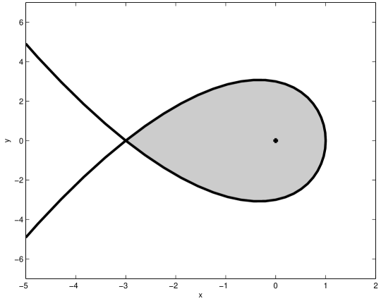
Figure 1: Frequency response of a stable third degree polynomial. The shaded region is the convex component containing the origin.

The Bézoutian matrices of Lemma 3 can be computed with the following Maple 10 instructions:

> with(LinearAlgebra):
> qx:=1-w^2:qy:=4*w-w^3:qz:=1:
> Bxy:=BezoutMatrix(qx,qy,w,method=symmetric);
                                   [-1     0     1]
                                   [              ]
                            Bxy := [ 0    -3     0]
                                   [              ]
                                   [ 1     0    -4]

> Byz:=BezoutMatrix(qy,qz,w,method=symmetric);
                                   [ 0     0     1]
                                   [              ]
                            Byz := [ 0     1     0]
                                   [              ]
                                   [ 1     0    -4]
> Bxz:=subs(e=0,BezoutMatrix(qx,qz+e*w^3,w,method=symmetric));
                                   [ 0     0     0]
                                   [              ]
                            Bxz := [ 0     0    -1]
                                   [              ]
                                   [ 0    -1     0]

Note the use of the subs instruction to ensure that the last Bézoutian matrix has appropriate dimension 3. Matrix $B(q_{x},q_{z})$ is negative definite, so a sign change is required to build

$$F(x,y)=\left[\begin{array}[]{ccc}1&0&-1+x\\ 0&3+x&-y\\ -1+x&-y&4-4x\end{array}\right]$$

and we obtain the following determinantal polynomial:

> F:=-(Bxy-x*Byz-y*Bxz);
> f:=Determinant(F);
                                           2    2    3
                         f := 9 - 3 x - 5 x  - y  - x

describing algebraic plane curve $\partial{\mathcal{P}}$ implicitly. The curve can be studied with the algcurves package of Maple:

> with(algcurves):
> genus(f,x,y);
                         0
> plot_real_curve(f,x,y);

4.2 Stable eighth degree polynomial

A more complicated example is the eighth degree stable polynomial $p(s)=336+198s+496s^{2}+117s^{3}+183s^{4}+20s^{5}+24s^{6}+s^{7}+s^{8}$ whose frequency response is represented on Figure 2. The rigidly convex region around the origin has the LMI description

$$\left[\begin{array}[]{c@{\;}c@{\;}c@{\;}c@{\;}c@{\;}c@{\;}c@{\;}c}1&0&-20&0&117&0&-198&y\\ 0&4&0&-66&0&298&y&-336+x\\ -20&0&414&0&-2510&y&4416+x&-24\,y\\ 0&-66&0&1150&y&-5504+x&-24\,y&6720-20\,x\\ 117&0&-2510&y&15907+x&-24\,y&-29514-20\,x&183\,y\\ 0&298&y&-5504+x&-24\,y&28518-20\,x&183\,y&-39312+117\,x\\ -198&y&4416+x&-24\,y&-29514-20\,x&183\,y&58896+117\,x&-496\,y\\ y&-336+x&-24\,y&6720-20\,x&183\,y&-39312+117\,x&-496\,y&66528-198\,x\end{array}\right]\succeq 0$$

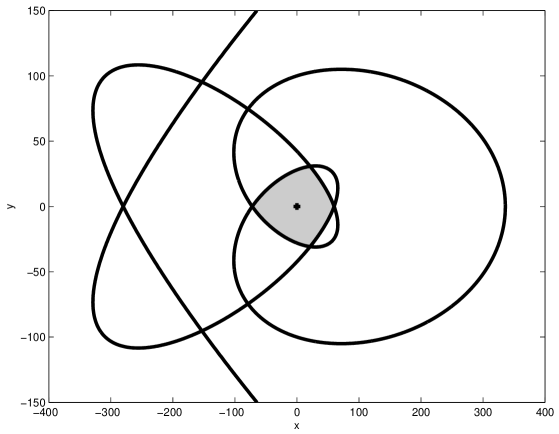
Figure 2: Frequency response of a stable eighth degree polynomial. The shaded region is rigidly convex.

4.3 Unstable fourth degree polynomial

This example is taken from [11]. Let $p(s)=s^{4}-s-1$. The implicit equation of $\partial{\mathcal{P}}$ is

$$f(x,y)=\det\>\left[\begin{array}[]{cccl}0&0&1&y\\ 0&1&y&0\\ 1&y&0&0\\ y&0&0&1+x\end{array}\right]=-1-x+y^{4}=0.$$

The component $\mathcal{P}$ including the origin is convex, see Figure 3, but it is not rigidly convex since a generic line passing through the origin cuts the quartic $\partial{\mathcal{P}}$ only twice. Hence this region does not admit an LMI representation, and by Theorem 1, polynomial $p(s)$ is unstable.

Note however that $\mathcal{P}$ can be represented as the projection of an LMI set:

$${\mathcal{P}}=\{x+jy:\>\exists z:\>\left[\begin{array}[]{cc}1+x&z\\ z&1\end{array}\right]\succeq 0,\>\left[\begin{array}[]{cc}z&y\\ y&1\end{array}\right]\succeq 0\}$$

by introducing a lifting variable $z$, but such constructions are out of the scope of this note.

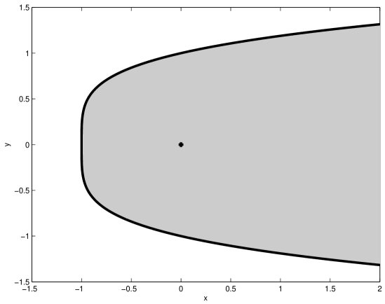
Figure 3: Frequency response of an unstable fourth degree polynomial. The shaded region is convex, but not rigidly convex.

5 Conclusion

Convexity of the connected component containing the origin and delimited by the frequency response of a stable polynomial was already established in [9]. In this note we give an alternative proof of this result based on Bézoutians and we give a more accurate characterization of the geometry of this region. Namely, the region is rigidly convex in the sense of [10], a property which is stronger than convexity, and which is equivalent to the existence of an LMI representation of the set.

In the terminology of convex analysis, the polynomial $f(x,y)$ defining implicitly the frequency response in (3) is hyperbolic with respect to the origin. Equivalently, $f(x,y)$ can be expressed as the determinant of a symmetric pencil which is positive definite at the origin. See [13] for a tutorial on hyperbolic polynomials and [12] for connections with the results of [10]. This note therefore unveils a link between polynomial hyperbolicity and stability.

References

- [1] S. S. Abhyankar. Algebraic geometry for scientists and engineers. AMS, 1990.
- [2] J. Ackermann. Robust control: the parameter space approach. Springer, 1993.
- [3] B. R. Barmish. New tools for robustness of linear systems. Macmillan, 1994.
- [4] S. Basu, R. Pollack, M.-F. Roy. Algorithms in real algebraic geometry. Springer, 2003.
- [5] S. P. Bhattacharyya, H. Chapellat, L. H. Keel. Robust control: the parametric approach. Prentice Hall, 1995.
- [6] D. Cox, J. Little, D. O’Shea. Ideals, varietes, and algorithms. Springer, 1992.
- [7] M. Elkadi, B. Mourrain. Introduction à la résolution des systèmes polynomiaux. Springer, 2007.
- [8] K. Gu. Comments on ”Convexity of frequency response arcs associated with a stable polynomial”. IEEE Trans. Autom. Control, 39(11):2262-2265, 1994.
- [9] J. C. Hamann, B. R. Barmish. Convexity of frequency response arcs associated with a stable polynomial. IEEE Trans. Autom. Control, 38(6):904-915, 1993.
- [10] J. W. Helton, V. Vinnikov. Linear matrix inequality representation of sets. Comm. Pure Applied Math. 60(5):654-674, 2007.
- [11] J. Kogan. Stability of a polynomial and convexity of a frequency response arc. Proc. IEEE Conf. on Decision and Control, 1993.
- [12] A. S. Lewis, P. A. Parrilo, M. V. Ramana. The Lax conjecture is true. Proc. Am. Math. Soc. 133(9):2495-2499, 2005.
- [13] J. Renegar. Hyperbolic programs and their derivative relaxations. Found. Comput. Math. 6(1): 59-79, 2006.
- [14] B. Sturmfels. Solving systems of polynomial equations. AMS, 2002.