The hydrodynamical relevance of the Camassa-Holm and Degasperis-Procesi equations

Abstract.

In recent years two nonlinear dispersive partial differential equations have attracted a lot of attention due to their integrable structure. We prove that both equations arise in the modeling of the propagation of shallow water waves over a flat bed. The equations capture stronger nonlinear effects than the classical nonlinear dispersive Benjamin-Bona-Mahoney and Korteweg-de Vries equations. In particular, they accomodate wave breaking phenomena.

1. Introduction

The study of water waves is a fascinating subject because the phenomena are familiar and the mathematical problems are various cf. [33]. Due to the relative intractability of the governing equations for water waves in regard to inferring from their direct study qualitative or quantitative conclusions about the propagation of waves at the water’s surface, from the earliest days in the development of hydrodynamics many competing models were suggested. Until the second half of the 20’th century, the study of water waves was confined almost exclusively to linear theory [12]. While linearisation gives insight for small perturbations on water initially at rest, its applicability fails for waves that are not small perturbations of a flat water surface. For example, linear water wave theory gives no insight into the study of phenomena which are manifestations of genuine nonlinear behaviour, like breaking waves breaking and solitary waves [31]. Many nonlinear models for water waves have been suggested to capture the existence of solitary water waves and the associated phenomenon of soliton manifestation [21]. The most prominent example is the Korteweg-de Vries (KdV) equation [23], the only member of the wider family of BBM-type equations [5] that is integrable and relevant for the phenomenon of soliton manifestation [15]. Another development of models for water waves was initiated in order to gain insight into wave breaking, one of the most fundamental aspects of water waves for which there appears to be no satisfactory mathematical theory [33]. Starting from the observation that the strong dispersive effect incorporated into the KdV model prevents wave breaking, Whitham (see the discussion in [33]) initiated the quest for equations that are simpler than the governing equations for water waves and which could model breaking waves. The physical validity of the first proposed models is questionable but two recently derived nonlinear integrable equations, the Camassa-Holm equation [7] and the Degasperis-Procesi equation [14], possess smooth solutions that develop singularities in finite time via a process that captures the essential features of breaking waves cf. [33]: the solution remains bounded but its slope becomes unbounded. Our aim is to prove the relevance of these two equations as models for the propagation of shallow water waves, proving that both are valid approximations to the governing equations for water waves. In our investigation we put earlier (formal) asymptotic procedures due to Johnson [22] on a firm and mathematically rigorous basis. We also investigate in what sense these two models give us insight into the wave breaking phenomenon by some simple numerical computations.

1.1. Unidirectional asymptotics for water waves

For one dimensional surfaces, the water waves equations read, in nondimensionalized form,

(1) $$\left\{\begin{array}[]{lcl}\mu\partial_{x}^{2}\Phi+\partial_{z}\Phi^{2}=0&\mbox{ in }&\Omega_{t},\\ \partial_{z}\Phi=0,&\mbox{ at }&z=0,\\ \partial_{t}\zeta-\frac{1}{\mu}(-\mu\partial_{x}\zeta\partial_{x}\Phi+\partial_{z}\Phi)=0&\mbox{ at }&z=\varepsilon\zeta,\\ \partial_{t}\Phi+\frac{\varepsilon}{2}(\partial_{x}\Phi)^{2}+\frac{\varepsilon}{2\mu}(\partial_{z}\Phi)^{2}=0&\mbox{ at }&z=\varepsilon\zeta,\end{array}\right.$$

where $x\mapsto\varepsilon\zeta(t,x)$ parameterizes the elevation of the free surface at time $t$, $\Omega_{t}=\{(x,z),-1<z<\varepsilon\zeta(t,x)\}$ is the fluid domain delimited by the free surface and the flat bottom $\{z=-1\}$, and where $\Phi(t,\cdot)$ (defined on $\Omega_{t}$) is the velocity potential associated to the flow (that is, the two-dimensional velocity field ${\bf v}$ is given by ${\bf v}=(\partial_{x}\Phi,\partial_{z}\Phi)^{T}$). Finally, $\varepsilon$ and $\mu$ are two dimensionless parameters defined as

$$\varepsilon=\frac{a}{h},\qquad\mu=\frac{h^{2}}{\lambda^{2}},$$

where $h$ is the mean depth, $a$ is the typical amplitude and $\lambda$ the typical wavelength of the waves under consideration. Making assumptions on the respective size of $\varepsilon$ and $\mu$, one is led to derive (simpler) asymptotic models from (1).
In the shallow-water scaling ($\mu\ll 1$), one can derive the so-called Green-Naghdi equations (see [19] for the derivation, and [3] for a rigorous justification), without any assumption on $\varepsilon$ (that is, $\varepsilon=O(1)$). For one dimensional surfaces and flat bottoms, these equations couple the free surface elevation $\zeta$ to the vertically averaged horizontal component of the velocity,

(2) $$u(t,x)=\frac{1}{1+\varepsilon\zeta}\int_{-1}^{\varepsilon\zeta}\partial_{x}\phi(t,x,z)dz;$$

and can be written as

(3) $$\left\{\begin{array}[]{l}\zeta_{t}+\big{[}(1+\varepsilon\zeta)u\big{]}_{x}=0\\ u_{t}+\zeta_{x}+\varepsilon uu_{x}=\frac{\mu}{3}\frac{1}{1+\varepsilon\zeta}\big{[}(1+\varepsilon\zeta)^{3}(u_{xt}+\varepsilon uu_{xx}-\varepsilon u_{x}^{2})\big{]}_{x},\end{array}\right.$$

where $O(\mu^{2})$ terms have been discarded.
If we make the additionnal assumption that $\varepsilon\ll 1$, then the above system reduces at first order to a wave equation of speed $\pm 1$ and any perturbation of the surface splits up into two components moving in opposite directions. A natural issue is therefore to describe more accurately the motion of these two “unidirectional” waves. In the so-called long-wave regime

(4) $$\mu\ll 1,\qquad\varepsilon=O(\mu),$$

Korteweg and de Vries [23] found that, say, the right-going wave should satisfy the KdV equation

$$u_{t}+u_{x}+\varepsilon\frac{3}{2}uu_{x}+\mu\frac{1}{6}u_{xxx}=0$$

(and $\zeta=u+O(\varepsilon,\mu)$), which at leading order reduces to the expected transport equation at speed $1$. More recently, it has been noticed by Benjamin, Bona, Mahoney [5] that the KdV equation belongs to a wider class of equations (the BBM equations, first used by Peregrine [29] and sometimes also called the regularized long-wave equations) which provide an approximation of the exact water waves equations of the same accuracy as the KdV equation:

(5) $$u_{t}+u_{x}+\frac{3}{2}\varepsilon uu_{x}+\mu(\alpha u_{xxx}+\beta u_{xxt})=0,\quad\mbox{ with }\quad\alpha-\beta=\frac{1}{6}.$$

The equations (5) contain both nonlinear effects (the $uu_{x}$ term) and dispersive effects (the $u_{xxx}$and $u_{xxt}$ terms) due to the scaling (4). However, these equations do not account correctly for large amplitude waves, whose behavior is more nonlinear than dispersive. For such waves, characterized by larger values of $\varepsilon$, it is natural to investigate the following scaling (which we call Camassa-Holm scaling):

(6) $$\mu\ll 1,\qquad\varepsilon=O(\sqrt{\mu}).$$

With this scaling, one still has $\varepsilon\ll 1$ and thus the same reduction to a simple wave equation at leading order; the dimensionless parameter is however larger here than in the long wave scaling, and the nonlinear effects are therefore stronger. In particular, a stronger nonlinearity could allow the appearance of breaking waves - a fundamental phenomenon in the theory of water waves that is not captured by the BBM equations. We show in this paper that the correct generalization of the BBM equations (5) under the scaling (6) is provided by the following class of equations:

(7) $$u_{t}+u_{x}+\frac{3}{2}\varepsilon uu_{x}+\mu(\alpha u_{xxx}+\beta u_{xxt})=\varepsilon\mu(\gamma uu_{xxx}+\delta u_{x}u_{xx})$$

(with some conditions on $\alpha$, $\beta$, $\gamma$ and $\delta$).
Notice that for an equation of the family (7) to be well-posed it is necessary that $\beta\leq 0$, as one can see by analyzing the linear part via Fourier transforms.

We want to insist on the fact that (7) provides an approximation of the same order $O(\mu^{2})$ as the BBM equations (5) to the Green-Naghdi equations. The only difference in the derivation of these equations lies in the different scalings (4) and (6). Since of course $O(\mu)=O(\sqrt{\mu})$ when $\mu$ is small, the long-wave scaling (4) is contained in the CH scaling (6), and consequently, the BBM equations can be recovered as a specialization of (7) when $\varepsilon=O(\mu)$ and not only $O(\sqrt{\mu})$.

1.2. The Camassa-Holm and Degasperis-Procesi equations

Among the various type of equations (7) with $\beta\leq 0$ there are only two with a bi-Hamiltonian structure: the Camassa-Holm and the Degasperis-Procesi equations [20]. Notice that while the KdV equation has a bi-Hamiltonian structure (see [15]), this is not the case for the other members of the BBM family of equations (5). The importance of a bi-Hamiltonian structure lies in the fact that in general it represents the hallmark of a completely integrable Hamiltonian system whose solitary wave solutions are solitons, that is, localized waves that recover their shape and speed after interacting nonlinearly with another wave of the same type (see [15, 21]).

1.2.1. Camassa-Holm equations

The Camassa-Holm (CH) equations are usually written under the form

(8) $$U_{t}+\widehat{\kappa}U_{x}+3UU_{x}-U_{txx}=2U_{x}U_{xx}+UU_{xxx},$$

with $\widehat{\kappa}\in\mathbb{R}$. A straightforward scaling argument shows that if $\widehat{\kappa}\neq 0$, (8) can be written under the form (7) by setting $u(t,x)=aU(b(x-vt),ct)$ and $a=\frac{2}{\varepsilon\widehat{\kappa}}$, $b^{2}=-\frac{1}{\beta\mu}$, $v=\frac{\alpha}{\beta}$, $c=\frac{b}{\widehat{\kappa}}(1-v)$ (which requires $\beta<0$ and leads to $\gamma=-\frac{\beta}{2}$ and $\delta=2\gamma$). This motivates the following definition:

Definition 1.

We say that (7) is a Camassa-Holm equation if the following conditions hold:

$$\beta<0,\quad\alpha\neq\beta,\quad\beta=-2\gamma,\quad\delta=2\gamma.$$

For all $\widehat{\kappa}\neq 0$, the solution $u$ to (7) is transformed into a solution $U$ to (8) by the transformation

$$U(t,x)=\frac{1}{a}u(\frac{x}{b}+\frac{v}{c}t,\frac{t}{c}),$$

with $a=\frac{2}{\varepsilon\widehat{\kappa}}(1-v)$, $b^{2}=-\frac{1}{\beta\mu}$, $v=\frac{\alpha}{\beta}$, and $c=\frac{b}{\widehat{\kappa}}(1-v)$.

First derived as a bi-Hamiltonian system by Fokas & Fuchssteiner [17], the equation (8) gained prominence after Camassa-Holm [7] independently re-derived it as an approximation to the Euler equations of hydrodynamics and discovered a number of the intriguing properties of this equation. In [7] a Lax pair formulation of (8) was found, a fact which lies at the core of showing via direct and inverse scattering [8, 10] that (8) is a completely integrable Hamiltonian system: for a large class of initial data, solving (8) amounts to integrating an infinite number of linear first-order ordinary differential equations which describe the evolution in time of the action-angle variables. The Camassa-Holm equations shares with KdV this integrability property as well as the fact that its solitary waves are solitons [11, 10]. We refer to [15] for a discussion of these properties in the context of the KdV model.

1.2.2. Degasperis-Procesi equations

The Degasperis-Procesi (DP) equations are usually written under the form

(9) $$U_{t}+\widehat{\kappa}U_{x}+4UU_{x}-U_{txx}=3U_{x}U_{xx}+UU_{xxx},$$

with $\widehat{\kappa}\in\mathbb{R}$. The same scaling arguments as for the CH equation motivate the following definition:

Definition 2.

We say that (7) is a Degasperis-Procesi equation if the following conditions hold:

$$\beta<0,\quad\alpha\neq\beta,\quad\beta=-\frac{8}{3}\gamma\quad\delta=3\gamma.$$

For all $\widehat{\kappa}\neq 0$, the solution $u$ to (7) is transformed into a solution $U$ to (9) by the transformation

$$U(t,x)=\frac{1}{a}u(\frac{x}{b}+\frac{v}{c}t,\frac{t}{c}),$$

with $a=\frac{8}{3\varepsilon\widehat{\kappa}}(1-v)$, $b^{2}=-\frac{1}{\beta\mu}$, $v=\frac{\alpha}{\beta}$ and $c=\frac{b}{\widehat{\kappa}}(1-v)$.

Equation (9), first derived in [14], is also known to have a Lax pair formulation [13] and its solitary waves interact like solitons [26]. Just like the KdV equation (see [15]) and the Camassa-Holm equation (see [24]), the Degasperis-Procesi equation has infinitely many integrals of motion.

1.3. Wave breaking

In addition to the properties of (8) and (9) mentioned before, the importance of these two equations is enhanced by their relevance to the modeling of wave breaking, one of the most important but mathematically still quite elusive phenomena encountered in the study of water waves.

Definition 3.

We say that there is wave breaking for an equation of the form (7), if there exists a time $0<t^{\varepsilon,\mu}<\infty$ and solutions $u$ to (7) such that

$$u\in L^{\infty}([0,t^{\varepsilon,\mu}]\times\mathbb{R})\quad\mbox{ and }\quad\lim_{t\to t^{\varepsilon,\mu}}|\partial_{x}u(t,\cdot)|_{\infty}=\infty.$$

The rationale of this definition is that if the flow velocity $u$ is to first order a good approximation to the surface profile $\zeta$, it is then reasonable to expect that the above blow-up pattern has a similar counterpart in terms of $\zeta$. If this were the case, the boundedness of the wave height in combination with an unbounded slope captures the main features of a breaking wave [33].

For KdV in particular, as well as for any other member of the BBM family (5), all smooth initial data $u(0,\cdot)$ decaying at infinity develop into solutions defined for all times (see e.g. [32]) so that the BBM family [5] does not model wave breaking [2, 30]. To remedy this shortcoming of the KdV equation Whitham proposed to formally replace the dispersive term $u_{xxx}$ by a convolution with a singular function chosen so that the newly obtained equation presents wave breaking (see [18, 33]). However, this formal process destroys the integrability and soliton features of the KdV equation. In contrast to this, both (8) and (9) admit breaking waves in the sense of Definition 3 cf. [6, 9, 27, 28] for (8) and [16] for (9). In this paper we explore the wave breaking phenomenon for both equations not in the restricted sense provided by Definition 3 but by studying the nonlinear equation describing the evolution in time of the free surface. While our results vindicate the fact that it is appropriate to use in this context Definition 3 to describe breaking waves, there is a slight twist. To be more precise, let us distinguish between two types of breaking waves that can be observed. In a plunging breaker the slope of the wave approaches $-\infty$ at the breaking location as we reach breaking time, while in a surging breaker the slope becomes $+\infty$. Considering the case of the Camassa-Holm equation (8), due to the fact that singularities in a smooth solution can appear only if $\inf_{x\in\mathbb{R}}\,\{u_{x}(t,x)\}\to-\infty$ as we approach breaking time while $\sup_{x\in\mathbb{R}}\,\{|u(t,x)|\}$ remains uniformly bounded (see [8]), we would expect to observe a plunging breaker at the free surface. However, as we recall here, the Camassa-Holm equation describes the behavior of the vertically averaged horizontal component of the velocity $u$; the free surface elevation $\zeta$ can be given in terms of $u$ ($\zeta=u+\frac{\varepsilon}{4}u^{2}+\mu\frac{1}{6}u_{xt}+O(\varepsilon\mu)$, see Proposition 1 below) but such an asymptotic expression of course breaks down when $u_{x}$ becomes singular, and cannot be used to describe the behavior of the free surface when there is “wave breaking” for the velocity. Since “wave breaking” is a very intuitive notion when it refers to the free surface elevation, we show in this article that it is possible to revert the usual approach; that is, we derive an evolution equation for the surface elevation $\zeta$ and give an asymptotic expression for the velocity $u$ in terms of $\zeta$ (cf. §2.2). This allows us to prove that wave breaking indeed occurs for the surface elevation but that, as opposed to what happens for the velocity, this is a surging breaker! The difference between plunging and surging breakers is graphically illustrated by numerical computations in §3.4.

2. Derivation of asymptotical equations for the unidirectional limit of the Green-Naghdi equations

We derive here asymptotical equations to the Green-Naghdi equations in the Camassa-Holm scaling (6). We recall that the Green-Naghdi equations are given by

$$\left\{\begin{array}[]{l}\zeta_{t}+\big{[}(1+\varepsilon\zeta)u\big{]}_{x}=0\\ u_{t}+\zeta_{x}+\varepsilon uu_{x}=\frac{\mu}{3}\frac{1}{1+\varepsilon\zeta}\big{[}(1+\varepsilon\zeta)^{3}(u_{xt}+\varepsilon uu_{xx}-\varepsilon u_{x}^{2})\big{]}_{x}.\end{array}\right.$$

Since we work under the Camassa-Holm scaling, we restrict our attention to values of $\varepsilon$ and $\mu$ satisfying

(10) $$(\varepsilon,\mu)\in{\mathcal{P}}:=\{\mu\in(0,\mu_{0}),\varepsilon\leq M\sqrt{\mu}\},$$

for some $\mu_{0}>0$ and $M>0$. Equations for the velocity $u$ (including the CH and DP equations) are first derived in §2.1, and equations for the surface elevation $\zeta$ are obtained in §2.2. The considerations we make on the derivation of these equations are related to the approach initiated by Johnson [22], approach that is substantiated and extended by our analysis. In addition, we explore the wave breaking phenomenon.

2.1. Equations on the velocity

At leading order, the Green-Naghdi equations degenerate into a simple wave equation of speeds $\pm 1$; including the $O(\varepsilon)$ terms, one can easily check that the (say) right-going component of the wave must satisfy

(11) $$u_{t}+u_{x}+\frac{3}{2}\varepsilon uu_{x}=0,$$

and $\zeta=u+O(\varepsilon)$.
If we want to find an asymptotic at order $O(\mu^{2})$ (recall that $\varepsilon=O(\mu^{1/2})$), it is therefore natural to look for $u$ as a solution of a perturbation of (11) including terms of order $O(\mu)$ and $O(\varepsilon\mu)$ similar to those present in (3). Thus we want $u$ to solve an equation of the form (7) where $\alpha$, $\beta$, $\gamma$ and $\delta$ are coefficients to be determined. We prove in this section that under certain conditions on the coefficients, one can associate to the solutions of (7) a family of approximate solutions consistent with the Green-Naghdi equations (3) in the following sense:

Definition 4.

Let $\mu_{0}>0$, $M>0$, $T>0$ and ${\mathcal{P}}$ be as defined in (10).
A family $(\zeta^{\varepsilon,\mu},u^{\varepsilon,\mu})_{(\varepsilon,\mu)\in{\mathcal{P}}}$ is consistent (of order $s\geq 0$ and on $[0,\frac{T}{\varepsilon}]$) with the Green-Naghdi equations (3) if for all $(\varepsilon,\mu)\in{\mathcal{P}}$,

$$\left\{\begin{array}[]{l}\zeta_{t}+\big{[}(1+\varepsilon\zeta)u\big{]}_{x}=\mu^{2}r_{1}^{\varepsilon,\mu}\\ u_{t}+\zeta_{x}+\varepsilon uu_{x}=\frac{\mu}{3}\frac{1}{1+\varepsilon\zeta}\big{[}(1+\varepsilon\zeta)^{3}(u_{xt}+\varepsilon uu_{xx}-\varepsilon u_{x}^{2})\big{]}_{x}+\mu^{2}r_{2}^{\varepsilon,\mu};\end{array}\right.$$

with $(r_{1}^{\varepsilon,\mu},r_{2}^{\varepsilon,\mu})_{(\varepsilon,\mu)\in{\mathcal{P}}}$ bounded in $L^{\infty}([0,\frac{T}{\varepsilon}],H^{s}(\mathbb{R})^{2})$.

The following proposition shows that there is a one parameter family of equations of the form (7) consistent with the Green-Naghdi equations.

Proposition 1.

Let $p\in\mathbb{R}$ and asssume that

$$\alpha=p,\quad\beta=p-\frac{1}{6},\quad\gamma=-\frac{3}{2}p-\frac{1}{6},\quad\delta=-\frac{9}{2}p-\frac{23}{24}.$$

Then there exists $D>0$ such that:

• For all $s\geq 0$ and $T>0$,

• For all bounded family $(u^{\varepsilon,\mu})_{(\varepsilon,\mu)\in{\mathcal{P}}}\in C([0,\frac{T}{\varepsilon}];H^{s+D}(\mathbb{R}))$ solving (7),

the family $(\zeta^{\varepsilon,\mu},u^{\varepsilon,\mu})_{(\varepsilon,\mu)\in{\mathcal{P}}}$, with (omitting the indexes $\varepsilon,\mu$)

$$\zeta:=u+\frac{\varepsilon}{4}u^{2}+\mu\frac{1}{6}u_{xt}-\varepsilon\mu\big{[}\frac{1}{6}uu_{xx}+\frac{5}{48}u_{x}^{2}\big{]},$$

is consistent (of order $s$ and on $[0,\frac{T}{\varepsilon}]$) with the Green-Naghdi equations (3).

Remark 1.

i. One can recover the equations (26a) and (26b) of [22] with $p=-\frac{1}{12}$ (and thus $\alpha=-\frac{1}{12}$, $\beta=-\frac{1}{4}$, $\gamma=-\frac{1}{24}$ and $\delta=-\frac{7}{12}$) and $p=\frac{1}{6}$ (and thus $\alpha=\frac{1}{6}$, $\beta=0,$ $\gamma=-\frac{5}{12}$ and $\delta=-\frac{41}{24}$) respectively.
ii. The one parameter family of equations (7) considered in the proposition admits only one representant for which $\delta=2\gamma$ (obtained for $p=-\frac{5}{12}$, and thus $\gamma=\frac{11}{24},$ $\delta=\frac{11}{12}$). However, since $\beta=-\frac{7}{12}\neq-2\gamma$, the corresponding equation is not a Camassa-Holm equation in the sense of Definition 1.
iii. There is no possible choice of $p$ such that $\delta=3\gamma$ in Proposition 1. Consequently, none of this one parameter family of equations is a Degasperis-Procesi equation. Notice that among all equations (7) with $\beta\leq 0$ there are only two with a bi-Hamiltonian structure: the Camassa-Holm and the Degasperis-Procesi equations [20].

Proof.

For the sake of simplicity, we use the notation $O(\mu)$, $O(\mu^{2})$, etc., without explicit mention to the functional normed space to which we refer. A precise statement has been given in Definition 4; it would be straightforward but quite heavy to maintain this formalism throughout the proof.
Step 1. If $u$ solves (7) then one also has

(12) $$u_{t}+u_{x}+\varepsilon\frac{3}{2}uu_{x}+\mu au_{xxt}=\varepsilon\mu\big{[}buu_{xx}+cu_{x}^{2}\big{]}_{x}+O(\mu^{2}),$$

with $a=\beta-\alpha$, $b=\gamma+\frac{3}{2}\alpha$ and $c=\frac{1}{2}(\delta+3\alpha-\gamma)$.
Differentiating (7) twice with respect to $x$, one gets indeed

$$u_{xxx}=-u_{xxt}-\frac{3}{2}\varepsilon\partial_{x}^{2}(uu_{x})+O(\mu),$$

and we can replace the $u_{xxx}$ term of (7) by this expression to get (12).

Step 2. We seek $v$ such that if $\zeta=u+\varepsilon v$ and $u$ solves (7) then the second equation of (3) is satisfied ut to a $O(\mu^{2})$ term. This is equivalent to checking that

$$u_{t}+[u+\varepsilon v]_{x}+\varepsilon uu_{x}-\frac{\mu}{3}u_{xxt} = \frac{\varepsilon\mu}{3}\big{[}-uu_{xxt}+[3uu_{xt}+uu_{xx}-u_{x}^{2}]_{x}\big{]}+O(\mu^{2}),$$

$$= -\frac{\varepsilon\mu}{3}\big{[}uu_{xx}+\frac{3}{2}u_{x}^{2}\big{]}_{x}+O(\mu^{2})$$

the last line being a consequence of the identity $u_{t}=-u_{x}+O(\varepsilon)$ provided by (12). The above equation can be recast under the form:

$$\varepsilon v_{x}+\big{[}u_{t}+u_{x}+\varepsilon\frac{3}{2}uu_{x}+\mu au_{xxt}-\varepsilon\mu\big{[}buu_{xx}+cu_{x}^{2}\big{]}_{x}\big{]}$$

$$=\frac{\varepsilon}{2}uu_{x}+\mu(a+\frac{1}{3})u_{xxt}-\varepsilon\mu\big{[}(b+\frac{1}{3})uu_{xx}+(c+\frac{1}{2})u_{x}^{2}\big{]}_{x}+O(\mu^{2}).$$

From Step 1, we know that the term between brackets in the lhs of this equation is of order $O(\mu^{2})$, so that that the second equation of (3) is satisfied up to $O(\mu^{2})$ terms if

$$\varepsilon v_{x}=\frac{\varepsilon}{2}uu_{x}+\mu(a+\frac{1}{3})u_{xxt}-\varepsilon\mu\big{[}(b+\frac{1}{3})uu_{xx}+(c+\frac{1}{2})u_{x}^{2}\big{]}_{x}+O(\mu^{2}),$$

so that we can take

(13) $$\varepsilon v=\frac{\varepsilon}{4}u^{2}+\mu(a+\frac{1}{3})u_{xt}-\varepsilon\mu\big{[}(b+\frac{1}{3})uu_{xx}+(c+\frac{1}{2})u_{x}^{2}\big{]}.$$

Step 3. We choose the coefficients $\beta$, $\gamma$ and $\mu$ such that the first equation of (3) is also satisfied up to $O(\mu^{2})$ terms. This is equivalent to checking that

(14) $$[u+\varepsilon v]_{t}+[(1+\varepsilon u)u]_{x}+\varepsilon^{2}[vu]_{x}=O(\mu^{2}).$$

First remark that one infers from (13) that

$$\varepsilon\partial_{t}v = \frac{\varepsilon}{2}uu_{t}+\mu(a+\frac{1}{3})u_{xtt}-\varepsilon\mu\big{[}(b+\frac{1}{3})uu_{xx}+(c+\frac{1}{2})u_{x}^{2}\big{]}_{t}.$$

$$= -\frac{\varepsilon}{2}u(u_{x}+\varepsilon\frac{3}{2}uu_{x}+\mu au_{xxt})-\mu(a+\frac{1}{3})\partial_{xt}^{2}(u_{x}+\varepsilon\frac{3}{2}(uu_{x}))$$

$$+\varepsilon\mu\big{[}(b+\frac{1}{3})uu_{xx}+(c+\frac{1}{2})u_{x}^{2}\big{]}_{x}+O(\mu^{2})$$

$$= -\varepsilon\frac{1}{2}uu_{x}-\varepsilon^{2}\frac{3}{4}u^{2}u_{x}-\mu(a+\frac{1}{3})u_{xxt}$$

$$+\varepsilon\mu\big{[}(2a+b+\frac{5}{6})uu_{xx}+(\frac{5}{4}a+c+1)u_{x}^{2}\big{]}_{x}+O(\mu^{2});$$

similarly, one gets

$$\varepsilon^{2}[vu]_{x}=\varepsilon^{2}\frac{3}{4}u^{2}u_{x}-\varepsilon\mu(a+\frac{1}{3})\big{[}uu_{xx}\big{]}_{x}+O(\mu^{2}),$$

so that (14) is equivalent to

$$u_{t}+u_{x}+\varepsilon\frac{3}{2}uu_{x}-\mu\varepsilon(a+\frac{1}{3})u_{xxt}=\varepsilon\mu\big{[}-(a+b+\frac{1}{2})uu_{xx}-(\frac{5}{4}a+c+1)u_{x}^{2}\big{]}+O(\mu^{2}).$$

Equating the coefficients of this equation with those of (12) shows that the first equation of (3) is also satisfied at order $O(\mu^{2})$ if the following relations hold:

$$a=-\frac{1}{6},\qquad b=-\frac{1}{6},\quad c=-\frac{19}{48},$$

and the conditions given in the statement of the proposition on $\alpha$, $\beta$, $\gamma$ and $\delta$ follows from the expressions of $a$, $b$ and $c$ given after equation (12). ∎

As said in Remark 1, none of the equations of the one parameter family considered in Proposition 1 is completely integrable. This is the reason why we now want to derive a wider class of equations of the form (7) – and whose solution can still be used as the basis of an approximate solution of the Green-Naghdi equations (3) (and thus of the water waves problem). We can generalize Proposition 1 by replacing the vertically averaged velocity $u$ given by (2) by the horizontal velocity $u^{\theta}$ ($\theta\in[0,1]$) evaluated at the level line $\theta$ of the fluid domain:

$$u^{\theta}(x)=\partial_{x}\Phi_{|_{z=(1+\varepsilon\zeta)\theta-1}},$$

so that $\theta=0$ and $\theta=1$ correspond to the bottom and surface respectively. The introduction of $\theta$ allows us to derive an approximation consistent with (3) built on a two-parameter family of equations of the form (7).

Proposition 2.

Let $p\in\mathbb{R}$, $\theta\in[0,1]$, and write $\lambda=\frac{1}{2}(\theta^{2}-\frac{1}{3})$. Asssuming that

$$\alpha=p+\lambda,\quad\beta=p-\frac{1}{6}+\lambda,\quad\gamma=-\frac{3}{2}p-\frac{1}{6}-\frac{3}{2}\lambda,\quad\delta=-\frac{9}{2}p-\frac{23}{24}-\frac{3}{2}\lambda,$$

there exists $D>0$ such that:

• For all $s\geq 0$ and $T>0$,

• For all bounded family $(u^{\varepsilon,\mu,\theta})_{(\varepsilon,\mu)\in{\mathcal{P}}}\in C([0,\frac{T}{\varepsilon}];H^{s+D}(\mathbb{R}))$ solving (7),

the family $(u^{\varepsilon,\mu},\zeta^{\varepsilon,\mu})_{(\varepsilon,\mu)\in{\mathcal{P}}}$, with (ommiting the indexes $\varepsilon,\mu$),

(15) $$u = u^{\theta}+\mu\lambda u^{\theta}_{xx}+2\mu\varepsilon\lambda u^{\theta}u^{\theta}_{xx},$$

(16) $$\zeta := u+\frac{\varepsilon}{4}u^{2}+\mu\frac{1}{6}u_{xt}-\varepsilon\mu\big{[}\frac{1}{6}uu_{xx}+\frac{5}{48}u_{x}^{2}\big{]},$$

is consistent (of order $s$ and on $[0,\frac{T}{\varepsilon}]$) with the Green-Naghdi equations (3).

Remark 2.

i. The one parameter family of equations (7) of Proposition 1 corresponds to the particular case $\theta^{2}=1/3$ (or $\lambda=0$).
ii. There exists only one set of coefficients such that $\delta=2\gamma$ and $\beta=-2\gamma$ (corresponding to $p=-\frac{1}{3}$ and $\theta^{2}=\frac{1}{2}$, and thus $\alpha=-\frac{1}{4}$, $\beta=-\frac{5}{12}<0$, $\gamma=\frac{5}{24}$, $\delta=\frac{5}{12}$). The corresponding equation is therefore a Camassa-Holm equation in the sense of Definition 1:

(17) $$u_{t}+u_{x}+\frac{3}{2}\varepsilon uu_{x}-\mu(\frac{1}{4}u_{xxx}+\frac{5}{12}u_{xxt})=\frac{5}{24}\varepsilon\mu(uu_{xxx}+2u_{x}u_{xx}).$$

iii. There exists only one set of coefficients such that $\delta=3\gamma$ and $\beta=-\frac{8}{3}\gamma$ (obtained with $\theta^{2}=\frac{23}{36}$ and $p=-\frac{77}{216}$, and thus $\alpha=-\frac{11}{54}$, $\beta=-\frac{10}{27}$, $\gamma=\frac{5}{36}$, $\delta=\frac{5}{12}$). The corresponding equation is therefore a Degasperis-Procesi equation in the sense of Definition 2:

$$u_{t}+u_{x}+\frac{3}{2}\varepsilon uu_{x}-\mu(\frac{11}{54}u_{xxx}+\frac{10}{27}u_{xxt})=\frac{5}{36}\varepsilon\mu(uu_{xxx}+3u_{x}u_{xx}).$$

Proof.

From the proof of Prop. 3.8 of [3], one has the following expression (neglecting terms of order $O(\mu^{2})$):

$$u = \partial_{x}\psi+\mu\big{(}(1+\varepsilon\zeta)\partial_{x}\zeta\partial_{x}\psi+\frac{(1+\varepsilon\zeta)^{2}}{3}\partial_{x}^{3}\psi\big{)},$$

$$u^{\theta} = \partial_{x}\psi+\mu\big{(}(1+\varepsilon\zeta)\partial_{x}\zeta\partial_{x}\psi+\frac{(1+\varepsilon\zeta)^{2}}{2}(1-\theta^{2})\partial_{x}^{3}\psi\big{)},$$

where $\psi$ denotes the trace of the velocity potential at the surface. It follows from these formulas that

$$u = u^{\theta}+\mu\frac{(1+\varepsilon\zeta)^{2}}{2}(\theta^{2}-\frac{1}{3})u^{\theta}_{xx}+O(\mu^{2})$$

$$= u^{\theta}+\mu\frac{1}{2}(\theta^{2}-\frac{1}{3})u^{\theta}_{xx}+\mu\varepsilon(\theta^{2}-\frac{1}{3})u^{\theta}u^{\theta}_{xx}+O(\mu^{2}),$$

where we used $\zeta=u^{\theta}+O(\varepsilon)$ for the last equality.
This formula, together with Proposition 1, easily yields the result. ∎

2.2. Equations on the surface elevation

Proceeding exactly as in the proof of Proposition 1, one can prove that the family of equations

(18) $$\zeta_{t}+\zeta_{x}+\frac{3}{2}\varepsilon\zeta\zeta_{x}-\frac{3}{8}\varepsilon^{2}\zeta^{2}\zeta_{x}+\frac{3}{16}\varepsilon^{3}\zeta^{3}\zeta_{x}+\mu(\alpha\zeta_{xxx}+\beta\zeta_{xxt})=\varepsilon\mu(\gamma\zeta\zeta_{xxx}+\delta\zeta_{x}\zeta_{xx})$$

for the evolution of the surface elevation can be used to construct an approximate solution consistent with the Green-Naghdi equations:

Proposition 3.

Let $q\in\mathbb{R}$ and asssume that

$$\alpha=q,\quad\beta=q-\frac{1}{6},\quad\gamma=-\frac{3}{2}q-\frac{1}{6},\quad\delta=-\frac{9}{2}q-\frac{5}{24}.$$

Then there exists $D>0$ such that:

• For all $s\geq 0$ and $T>0$,

• For all bounded family $(\zeta^{\varepsilon,\mu})_{(\varepsilon,\mu)\in{\mathcal{P}}}\in C([0,\frac{T}{\varepsilon}];H^{s+D}(\mathbb{R}))$ solving (18),

the family $(\zeta^{\varepsilon,\mu},u^{\varepsilon,\mu})_{(\varepsilon,\mu)\in{\mathcal{P}}}$, with (omitting the indexes $\varepsilon,\mu$)

$$u:=\zeta+\frac{1}{h}\Big{(}-\frac{\varepsilon}{4}\zeta^{2}-\frac{\varepsilon^{2}}{8}\zeta^{3}+\frac{\varepsilon^{3}}{64}\zeta^{4}-\mu\frac{1}{6}\zeta_{xt}+\varepsilon\mu\big{[}\frac{1}{6}\zeta\zeta_{xx}+\frac{1}{48}\zeta_{x}^{2}\big{]}\Big{)},$$

is consistent (of order $s$ and on $[0,\frac{T}{\varepsilon}]$) with the Green-Naghdi equations (3).

Remark 3.

Choosing $q=1/12$, the equation (18) reads

(19) $$\zeta_{t}+\zeta_{x}+\frac{3}{2}\varepsilon\zeta\zeta_{x}-\frac{3}{8}\varepsilon^{2}\zeta^{2}\zeta_{x}+\frac{3}{16}\varepsilon^{3}\zeta^{3}\zeta_{x}+\frac{\mu}{12}(\zeta_{xxx}-\zeta_{xxt})$$

$$\hskip 142.26378pt=-\frac{7}{24}\varepsilon\mu(\zeta\zeta_{xxx}+2\zeta_{x}\zeta_{xx}).$$

While for any $q\in\mathbb{R}$, (18) is an equation for the evolution of the free surface $\zeta$, and all these equations have the same order of accuracy $O(\varepsilon^{4},\mu^{2})$, it is more advantageous to use (19) since it presents better structural properties that we take advantage of in §3.3. The ratio $2:1$ between the coefficients of $\zeta_{x}\zeta_{xx}$ and $\zeta\zeta_{xxx}$ is crucial in our considerations.

3. Mathematical analysis of the models and rigorous justification

3.1. Large time well-posedness of the unidirectional equations (7) and (18)

We prove here the well posedness of the general class of equations

(20) $$u_{t}+u_{x}+\frac{3}{2}\varepsilon uu_{x}+\varepsilon^{2}\iota u^{2}u_{x}+\varepsilon^{3}\kappa u^{3}u_{x}+\mu(\alpha u_{xxx}+\beta u_{xxt})$$

$$\qquad=\varepsilon\mu(\gamma uu_{xxx}+\delta u_{x}u_{xx}),$$

with $\iota,\,\kappa\in\mathbb{R}$; in particular, (20) coincides with (7) and (18) if one takes $\iota=\kappa=0$ and $\iota=-\frac{3}{8}$, $\kappa=\frac{3}{16}$ respectively. That is, we solve the initial value problem

(21) $$\left|\begin{array}[]{l}u_{t}+u_{x}+\frac{3}{2}\varepsilon uu_{x}+\varepsilon^{2}\iota u^{2}u_{x}+\varepsilon^{3}\kappa u^{3}u_{x}+\mu(\alpha u_{xxx}+\beta u_{xxt})\\ \hskip 85.35826pt=\varepsilon\mu(\gamma uu_{xxx}+\delta u_{x}u_{xx}),\\ u_{|_{t=0}}=u^{0}\end{array}\right.$$

on a time scale $O(1/\varepsilon)$, and under the condition $\beta<0$. In order to state the result, we need to define the spaces $X^{s}$ as

$$\forall s\geq 0,\qquad X^{s+1}=H^{s+1}(\mathbb{R})\mbox{ endowed with the norm }|f|_{X^{s+1}}^{2}=|f|_{H^{s}}^{2}+\mu|\partial_{x}f|_{H^{s}}^{2},$$

and we also recall that the set ${\mathcal{P}}$ is defined in (10).

Proposition 4.

Assume that $\beta<0$ and let $\mu_{0}>0$, $M>0$, $s>\frac{3}{2}$ and $u^{0}\in H^{s+1}(\mathbb{R})$. Then, there exists $T>0$ and a unique family of solutions $(u_{\varepsilon,\mu})_{(\varepsilon,\mu)\in{\mathcal{P}}}$ to (21) bounded in $C([0,\frac{T}{\varepsilon}];X^{s+1}(\mathbb{R}))\cap C^{1}([0,\frac{T}{\varepsilon}];X^{s}(\mathbb{R}))$.

Proof.

For all $v$ smooth enough, let us define the “linearized” operator ${\mathcal{L}}(v,\partial)$ as

$${\mathcal{L}}(v,\partial) = (1+\mu\beta\partial_{x}^{2})\partial_{t}+\partial_{x}+\mu\alpha\partial_{x}^{3}+\frac{3}{2}\varepsilon v\partial_{x}+\varepsilon^{2}\iota v^{2}\partial_{x}+\varepsilon^{3}\kappa v^{3}\partial_{x}$$

$$-\varepsilon\mu\gamma v\partial_{x}^{3}-\varepsilon\mu\delta\big{(}\frac{1}{2}v_{x}\partial_{x}^{2}+\frac{1}{2}v_{xx}\partial_{x}\big{)},$$

In order to construct a solution to (20) by an iterative scheme, we are led to study the initial value problem

(22) $$\left\{\begin{array}[]{l}{\mathcal{L}}(v,\partial)u=\varepsilon f,\\ u_{|_{t=0}}=u^{0}.\end{array}\right.$$

If $v$ is smooth enough, it is completely standard to check that for all $s\geq 0$, $f\in L^{1}_{loc}(\mathbb{R}^{+}_{t};H^{s}(\mathbb{R}_{x}))$ and $u^{0}\in H^{s}(\mathbb{R})$, there exists a unique solution $u\in C(\mathbb{R}^{+};H^{s+1}(\mathbb{R}))$ to (22) (recall that $\beta<0$). We take for granted the existence of a solution to (22) and establish some precise energy estimates on the solution. In order to do so, let us define the “energy” norm

$$\forall s\geq 0,\qquad E^{s}(u)^{2}=|u|_{H^{s}}^{2}-\mu\beta|\partial_{x}u|_{H^{s}}^{2}.$$

Differentiating $\frac{1}{2}e^{-\varepsilon\lambda t}E^{s}(u)$ with respect to time, one gets, using the equation (22) and integrating by parts,

$$\frac{1}{2}e^{\varepsilon\lambda t}\partial_{t}(e^{-\varepsilon\lambda t}E^{s}(u)^{2}) = -\frac{\varepsilon\lambda}{2}E^{s}(u)^{2}+\varepsilon(\Lambda^{s}f,\Lambda^{s}u)-\varepsilon(\Lambda^{s}(V\partial_{x}u),\Lambda^{s}u)$$

$$+\varepsilon\mu\gamma(\Lambda^{s}(v\partial_{x}^{3}u),\Lambda^{s}u)-\varepsilon\mu\frac{\delta}{2}(\Lambda^{s}(v_{x}\partial_{x}u),\Lambda^{s}\partial_{x}u),$$

with $V=\frac{3}{2}v+\varepsilon\iota v^{2}+\varepsilon^{2}\kappa v^{3}$.
Since for all constant coefficient skewsymmetric differential polynomial $P$ (that is, $P^{*}=-P$), and all $h$ smooth enough, one has

$$(\Lambda^{s}(hPu),\Lambda^{s}u)=([\Lambda^{s},h]Pu,\Lambda^{s}u)-\frac{1}{2}([P,h]\Lambda^{s}u,\Lambda^{s}u),$$

we deduce (applying this identity with $P=\partial_{x}$ and $P=\partial_{x}^{3}$),

$$\frac{1}{2}e^{\varepsilon\lambda t}\partial_{t}(e^{-\varepsilon\lambda t}E^{s}(u)^{2})=-\frac{\varepsilon\lambda}{2}E^{s}(u)^{2}-\varepsilon\big{(}[\Lambda^{s},V]\partial_{x}u,\Lambda^{s}u)+\frac{\varepsilon}{2}((\partial_{x}V)\Lambda^{s}u,\Lambda^{s}u\big{)}$$

$$-\varepsilon\mu\gamma\big{(}[\Lambda^{s},v]\partial_{x}^{2}u-\frac{3}{2}v_{x}\Lambda^{s}\partial_{x}u-v_{xx}\Lambda^{s}u,\Lambda^{s}\partial_{x}u\big{)}-\varepsilon\mu\gamma\big{(}[\Lambda^{s},v_{x}]\partial_{x}^{2}u,\Lambda^{s}u\big{)}$$

$$-\varepsilon\mu\frac{\delta}{2}(\Lambda^{s}(v_{x}\partial_{x}u),\Lambda^{s}\partial_{x}u)+\varepsilon(\Lambda^{s}f,\Lambda^{s}u),$$

Here we also used the identities

$$[\Lambda^{s},v]\partial_{x}^{3}u=\partial_{x}\big{(}[\Lambda^{s},v]\partial_{x}^{2}u\big{)}-[\Lambda^{s},v_{x}]\partial_{x}^{2}u$$

and

$$\frac{1}{2}(v_{xxx}\Lambda^{s}u,\Lambda^{s}u)=-(v_{xx}\Lambda^{s}u,\Lambda^{s}u_{x}).$$

Since $|u|_{H^{s}}\leq E^{s}(u)$ and $\sqrt{\mu}|\partial_{x}u|_{H^{s}}\leq\frac{1}{\sqrt{-\beta}}E^{s}(u)$, one gets directly by the Cauchy-Schwartz inequality,

$$e^{\varepsilon\lambda t}\partial_{t}(e^{-\varepsilon\lambda t}E^{s}(u)^{2}) \leq \varepsilon C(\mu_{0},\frac{1}{\beta},\gamma,\delta)(A(u,v)E^{s}(u)+B(v)E^{s}(u)^{2})$$

$$-\varepsilon\lambda E^{s}(u)^{2}+2|f|_{H^{s}}E^{s}(u),$$

with

$$A(u,v) = |[\Lambda^{s},V]\partial_{x}u|_{2}+|[\Lambda^{s},v]\partial_{x}(\sqrt{\mu}\partial_{x}u)|_{2}+|[\Lambda^{s},\sqrt{\mu}v_{x}]\partial_{x}(\sqrt{\mu}\partial_{x}u)|_{2}$$

$$+\sqrt{\mu}|v_{x}\partial_{x}u|_{H^{s}},$$

$$B(v) = |\partial_{x}V|_{\infty}+|v_{x}|_{\infty}+|\partial_{x}(\sqrt{\mu}\partial_{x}v)|_{\infty}.$$

Recalling that for all $s>3/2$, and all $F,U$ smooth enough, one has

$$|[\Lambda^{s},F]U|_{2}\leq\mbox{{Cst }}|F|_{H^{s}}|U|_{H^{s-1}},$$

it is easy to check that one gets $A(u,v)\leq C(\mu_{0},M,\frac{1}{\beta},\iota,\kappa,E^{s}(v))E^{s}(u)$ and $B(v)\leq C(\mu_{0},M,\frac{1}{\beta},\iota,\kappa,E^{s}(v))$. Therefore, we obtain

$$e^{\varepsilon\lambda t}\partial_{t}(e^{-\varepsilon\lambda t}E^{s}(u)^{2})\leq\big{(}C(\mu_{0},M,\frac{1}{\beta},\gamma,\delta,\iota,\kappa,E^{s}(v))-\lambda\big{)}E^{s}(u)^{2}+2\varepsilon E^{s}(f)E^{s}(u).$$

Taking $\lambda=\lambda_{T}$ large enough (how large depending on $C(\mu_{0},M,\frac{1}{\beta},\gamma,\delta,\iota,\kappa,E^{s}(v))$) to have the first term of the right hand side negative for all $t\in[0,\frac{T}{\varepsilon}]$, one deduces

$$\forall t\in[0,\frac{T}{\varepsilon}],\qquad\partial_{t}(e^{-\varepsilon\lambda_{T}t}E^{s}(u)^{2})\leq 2\varepsilon e^{-\varepsilon\lambda_{T}t}E^{s}(f)E^{s}(u).$$

Integrating this differential inequality yields therefore

$$\forall t\in[0,\frac{T}{\varepsilon}],\qquad E^{s}(u)(t)\leq e^{\varepsilon\lambda_{T}t}E^{0}(u^{0})+2\varepsilon\int_{0}^{t}e^{\lambda_{T}(t-t^{\prime})}E^{s}(f(t^{\prime}))dt^{\prime}.$$

Thanks to this energy estimate, one can conclude classically (see e.g. [1]) to the existence of

$$T=T(\mu_{0},M,|u^{0}|_{X^{s+1}_{\mu_{0}}},\frac{1}{\beta},\gamma,\delta,\iota,\kappa)>0,$$

and of a unique solution $u\in C([0,\frac{T}{\varepsilon}];X^{s+1}(\mathbb{R}^{d}))$ to (21) as a limit of the iterative scheme

$$u_{0}=u^{0},\quad\mbox{ and }\quad\forall n\in\mathbb{N},\quad\left\{\begin{array}[]{l}{\mathcal{L}}(u^{n},\partial)u^{n+1}=0,\\ u^{n+1}_{|_{t=0}}=u^{0}.\end{array}\right.$$

Since $u$ solves (20), we have ${\mathcal{L}}(u,\partial u)u=0$ and therefore

$$(\Lambda^{s-1}(1+\mu\beta\partial_{x}^{2})\partial_{t}u,\Lambda^{s-1}\partial_{t}u)=-\varepsilon(\Lambda^{s-1}{\mathcal{M}}(u,\partial)u,\Lambda^{s-1}\partial_{t}u),$$

with ${\mathcal{M}}(u,\partial)={\mathcal{L}}(u,\partial)-(1+\mu\beta\partial_{x}^{2})\partial_{t}$. Proceeding as above, one gets

$$E^{s-1}(\partial_{t}u)\leq C(\mu_{0},M,|u^{0}|_{X^{s+1}_{\mu_{0}}},\frac{1}{\beta},\gamma,\delta,\iota,\kappa,E^{s}(u)),$$

and it follows that the family of solution is also bounded in $C^{1}([0,\frac{T}{\varepsilon}];X^{s})$. ∎

3.2. Rigorous justification of the unidirectional approximations (7)

In Proposition 2, we constructed a family $(u^{\varepsilon,\mu},\zeta^{\varepsilon,\mu})$ consistent with the Green-Naghdi equations in the sense of Definition 4. A consequence of the following theorem is a stronger result: this family provides a good approximation of the exact solutions $(\underline{u}^{\varepsilon,\mu},\underline{\zeta}^{\varepsilon,\mu})$ of the Green-Naghdi equations with same initial data in the sense that $(\underline{u}^{\varepsilon,\mu},\underline{\zeta}^{\varepsilon,\mu})=(u^{\varepsilon,\mu},\zeta^{\varepsilon,\mu})+O(\mu^{2}t)$ for times $O(1/\varepsilon)$.

Theorem 1.

Let $\mu_{0}>0$, $M>0$, $T>0$ and ${\mathcal{P}}$ be as defined in (10). Let also $p\in\mathbb{R}$, $\theta\in[0,1]$, and $\alpha$, $\beta$, $\gamma$ and $\delta$ be as in Proposition 2.
If $\beta<0$ then there exists $D>0$ and $T>0$ such that for all $u^{0}\in H^{s+D+1}(\mathbb{R})$:

• There is a unique family $(u^{\varepsilon,\mu},\zeta^{\varepsilon,\mu})_{(\varepsilon,\mu)\in{\mathcal{P}}}\in C([0,\frac{T}{\varepsilon}];H^{s+D}(\mathbb{R})^{2})$ given by the resolution of (7) with initial condition $u^{0}$ and formulas (15)-(16);

• There is a unique family $(\underline{u}^{\varepsilon,\mu},\underline{\zeta}^{\varepsilon,\mu})_{(\varepsilon,\mu)\in{\mathcal{P}}}\in C([0,\frac{T}{\varepsilon}];H^{s+D}(\mathbb{R})^{2})$ solving the Green-Naghdi equations (3) with initial condition $(u^{\varepsilon,\mu},\zeta^{\varepsilon,\mu})_{|_{t=0}}$.

Moreover, one has for all $(\varepsilon,\mu)\in{\mathcal{P}}$,

$$\forall t\in[0,\frac{T}{\varepsilon}],\qquad|\underline{u}^{\varepsilon,\mu}-u^{\varepsilon,\mu}|_{L^{\infty}([0,t]\times\mathbb{R})}+|\underline{\zeta}^{\varepsilon,\mu}-\zeta^{\varepsilon,\mu}|_{L^{\infty}([0,t]\times\mathbb{R})}\leq\mbox{{Cst }}\mu^{2}t.$$

Remark 4.

It is known (see [3]) that the Green-Naghdi equations give, under the scaling (6), a correct approximation of the exact solutions of the full water waves equations (with a precision $O(\mu^{2}t)$ and over a time scale $O(1/\varepsilon)$). It follows that that the unidirectional approximation discussed above approximates the solution of the water waves equations with the same accuracy.

Remark 5.

We used the unidirectional equations derived on the velocity as the basis for the approximation justified in the theorem. One could of course use instead the unidirectional approximation (18) derived on the surface elevation.

Proof.

The first point of the theorem is a direct consequence of Proposition 4. Thanks to Proposition 2, we now that $(u^{\varepsilon,\mu},\zeta^{\varepsilon,\mu})_{\varepsilon,\mu}$ is consistent with the Green-Naghdi equations (3), so that the second point of the theorem and the error estimate follow at once from the well-posedness and stability of the Green-Naghdi equations (see Th. 3 of [4]– note that instead of using this general result which holds for two dimensional surfaces and nonflat bottoms, one could easily adapt the simpler and more precise results of [25] to the present scaling). ∎

3.3. Wave breaking

For the Camassa-Holm family of equations (7) for the velocity it is known (see [8]) that singularities can develop in finite time for a smooth initial data only in the form of wave breaking. We will show now that this form of blow-up is also a feature of the equation (19) for the free surface. More precisely, if a smooth initial profile fails to produce a wave that exists for all subsequent times, then we encounter wave breaking in the form of surging (and not plunging, as would be the case if (7) were the equation for the evolution of the free surface).

Our first result describes the precise blow-up pattern for the equation (19) for the free surface.

Proposition 5.

Let $\zeta_{0}\in H^{3}(\mathbb{R})$. If the maximal existence time $T>0$ of the solution of (19) with initial profile $\zeta(0,\cdot)=\zeta_{0}$ is finite, $T<\infty$, then the solution $\zeta\in C^{1}([0,T);H^{2}(\mathbb{R}))\cap C([0,T);H^{(}\mathbb{R}))$ is such that

(23) $$\sup_{t\in[0,T),\,x\in\mathbb{R}}\{|\zeta(t,x)|\}<\infty$$

and

(24) $$\sup_{x\in\mathbb{R}}\,\{\zeta_{x}(t,x)\}\uparrow\infty\quad as\quad t\uparrow T.$$

Proof.

In view of Proposition 4, given $\zeta_{0}\in H^{3}(\mathbb{R})$, the maximal existence time of the solution $\zeta(t)$ to (19) with initial data $\zeta(0)=\zeta_{0}$ is finite if and only if $|\zeta(t)|_{H^{3}(\mathbb{R})}$ blows-up in finite time. Thus if (24) holds for some finite $T>0$, then the maximal existence time is finite. To complete the proof it suffices to show that

(i) the solution $\zeta(t)$ given by Proposition 4 remains uniformly bounded as long as it is defined;

and

(ii) if we can find some $M=M(\zeta_{0})>0$ such that

(25) $$\zeta_{x}(t,x)\leq M,\qquad x\in\mathbb{R},$$

as long as the solution is defined, then $|\zeta(t)|_{H^{3}(\mathbb{R})}$ stays bounded on bounded time-intervals.

Item (i) follows at once from the imbedding $L^{\infty}(\mathbb{R})\subset H^{1}(\mathbb{R})$ since multiplying (19) by $\zeta$ and integrating on $\mathbb{R}$ yields

(26) $$\partial_{t}\Big{(}\int_{\mathbb{R}}[\zeta^{2}+\frac{1}{12}\,\mu\int_{\mathbb{R}}\zeta_{x}^{2}]\,dx\Big{)}=0.$$

To prove item (ii), notice that multiplication of (19) by $\zeta_{xxxx}$ yields

(27) $$\partial_{t}\Big{(}\int_{\mathbb{R}}[\zeta_{xx}^{2}+\frac{1}{12}\,\mu\int_{\mathbb{R}}\zeta_{xxx}^{2}]\,dx\Big{)}=15\,\varepsilon\int_{\mathbb{R}}\zeta\zeta_{xx}\zeta_{xxx}\,d-\frac{15}{4}\,\varepsilon^{2}\int_{\mathbb{R}}\zeta^{2}\zeta_{xx}\zeta_{xxx}\,dx$$

$$\qquad+\frac{9}{16}\varepsilon^{3}\int_{\mathbb{R}}\zeta_{x}^{5}\,dx+\frac{15}{8}\,\varepsilon^{3}\int_{\mathbb{R}}\zeta^{3}\zeta_{xx}\zeta_{xxx}\,dx+\frac{7}{4}\,\mu\varepsilon\int_{\mathbb{R}}\zeta_{x}\zeta_{xxx}^{2}\,dx.$$

after performing several integrations by parts. If (25) holds, let in accordance with (26) the constant $M_{0}>0$ be such that

$$|\zeta(t,x)|\leq M_{0},\qquad x\in\mathbb{R},$$

for as long as the solution exists. Using the Cauchy-Schwartz inequality as well as the fact that $\mu\leq 1$, we infer from (26) and (27) that

$$\partial_{t}E(t)\leq\Big{(}\frac{90\varepsilon}{\mu}\,M_{0}+\frac{45\varepsilon^{2}}{2\mu}\,M_{0}^{2}+\frac{27\varepsilon^{3}}{4\mu}\,M^{3}+\frac{45\varepsilon^{3}}{4\mu}\,M_{0}^{3}+\,21\,\varepsilon M\Big{)}\,E(t),$$

where

$$E(t)=\int_{\mathbb{R}}[\zeta^{2}+\frac{1}{12}\,\mu\zeta_{x}^{2}+\zeta_{xx}^{2}+\frac{1}{12}\,\mu\zeta_{xxx}^{2}]\,dx.$$

An application of Gronwall’s inequality enables us to conclude. ∎

Our next aim is to show that there are solutions to (19) that blow-up in finite time as surging breakers, that is, following the pattern given in Proposition 5. We will prove this by analyzing the equation that describes the evolution of

(28) $$M(t)=\sup_{x\in\mathbb{R}}\,\{\zeta_{x}(t,x)\}.$$

For the degree of smoothness of the solution $\zeta(t)$ given by Proposition 4, we know that $M(t)$ is locally Lipschitz and

(29) $$\frac{d}{dt}\,M(t)=\zeta_{tx}(t,\xi(t))\quad\hbox{for a.e.}\quad t,$$

where $\xi(t)$ is any point where $M(t)=\zeta_{x}(t,\xi(t))$ cf. [9]. For further use, let us also note that

(30) $$(1-\frac{1}{12}\,\mu\,\partial_{x}^{2})^{-1}f=P\ast f,\qquad f\in L^{2}(\mathbb{R}),$$

where

$$P(x)=\sqrt{\frac{3}{\mu}}\ e^{-\displaystyle\,2\,\sqrt{\frac{3}{\mu}}\,|x|},\qquad x\in\mathbb{R},$$

with

(31) $$\|P\|_{L^{\infty}}=\sqrt{\frac{3}{\mu}},\quad\|P\|_{L^{1}}=1,\quad\|P\|_{L^{2}}=\Big{(}\frac{3}{4\mu}\Big{)}^{\frac{1}{4}},$$

and

(32) $$\quad\|P_{x}\|_{L^{\infty}}=\frac{6}{\mu},\quad\|P_{x}\|_{L^{1}}=2\,\sqrt{\frac{3}{\mu}},\quad\|P_{x}\|_{L^{2}}=\sqrt{2}\,\Big{(}\frac{3}{\mu}\Big{)}^{\frac{3}{4}}\leq 4\,\mu^{-\frac{3}{4}}.$$

Applying $(1-\frac{1}{12}\,\mu\,\partial_{x}^{2})^{-1}$ to (19), we obtain the equation

$$\zeta_{t}+P_{x}\ast\zeta+\frac{3}{4}\,\varepsilon\,P_{x}\ast\zeta^{2}-\frac{1}{8}\,\varepsilon^{2}\,P_{x}\ast\zeta^{3}+\frac{3}{64}\,\varepsilon^{3}\,P_{x}\ast\zeta^{4}$$

$$\qquad+\frac{1}{12}\,\mu\,\partial_{x}^{3}\,P\ast\zeta=-\frac{7}{24}\,\mu\varepsilon\,P_{x}\ast\zeta_{x}^{2}-\frac{7}{24}\,\mu\varepsilon\,P\ast(\zeta\zeta_{xxx}).$$

Differentiating this equation with respect to the spatial variable, we obtain

$$\zeta_{tx}+\partial_{x}^{2}P\ast\zeta+\frac{3}{4}\,\varepsilon\,\partial_{x}^{2}P\ast\zeta^{2}-\frac{1}{8}\,\varepsilon^{2}\,\partial_{x}^{2}P\ast\zeta^{3}+\frac{3}{64}\,\varepsilon^{3}\,\partial_{x}^{2}P\ast\zeta^{4}$$

$$\qquad+\frac{1}{12}\,\mu\,\partial_{x}^{4}\,P\ast\zeta=-\frac{7}{24}\,\mu\varepsilon\,\partial_{x}^{2}P\ast\zeta_{x}^{2}-\frac{7}{24}\,\mu\varepsilon\,P_{x}\ast(\zeta\zeta_{xxx}).$$

Since $\zeta\zeta_{xxx}=\partial_{x}^{2}(\zeta\zeta_{x})-3\zeta_{x}\zeta_{xx}$ and

(33) $$\partial_{x}^{2}\,P\ast f=P_{x}\ast\zeta_{x}=\frac{12}{\mu}\,P\ast f-\frac{12}{\mu}\,f,\qquad f\in L^{2}(\mathbb{R}),$$

we deduce that

(34) $$\zeta_{tx}+2\,P_{x}\ast\zeta_{x}-\frac{3}{8}\,\varepsilon^{2}\,P_{x}\ast(\zeta^{2}\zeta_{x})+\frac{3\varepsilon^{3}}{16}\,P_{x}\ast(\zeta^{3}\zeta_{x})$$

$$\qquad=\zeta_{xx}+\frac{7\varepsilon}{4}\,P\ast\zeta_{x}^{2}+\frac{7\varepsilon}{4}\,\zeta_{x}^{2}+\frac{7\varepsilon}{2}\,\zeta\zeta_{xx}-\frac{7}{2}\,\varepsilon\,P_{x}\ast(\zeta\zeta_{x}).$$

We can now prove the following blow-up result.

Proposition 6.

If the initial wave profile $\zeta_{0}\in H^{3}(\mathbb{R})$ satisfies

$$\Big{|}\sup_{x\in\mathbb{R}}\,\{\zeta_{0}(x)\}\Big{|}^{2} \geq \frac{28}{3}\,C_{0}\,\mu^{-3/4}+\frac{1}{2}\,\varepsilon\,C_{0}^{3/2}\,\mu^{-3/4}+\frac{1}{4}\,\varepsilon^{2}\,C_{0}^{2}\,\mu^{-3/4}$$

$$\qquad+\frac{7}{3}\,C_{0}\,\mu^{-1/2}+\frac{16}{3}\,C_{0}^{1/2}\,\mu^{-3/4}\,\varepsilon^{-1},$$

where

$$C_{0}=\int_{\mathbb{R}}[\zeta_{0}^{2}+(\zeta_{0}^{\prime})^{2}]\,dx>0,$$

then wave breaking occurs for the solution of (19) in finite time $T=O(\frac{1}{\varepsilon})$.

Proof.

Notice that

$$\sup_{x\in\mathbb{R}}\,\{|\zeta^{2}(x)|\}\leq\frac{1}{2}\,\int_{\mathbb{R}}(\zeta^{2}+\zeta_{x}^{2})\,dx=\frac{C_{0}}{2}.$$

Therefore, using Young’s inequality and the estimates (31)-(32), we obtain that

$$\|P_{x}\ast\zeta_{x}\|_{L^{\infty}}\leq\|P_{x}\|_{L^{2}}\|\zeta_{x}\|_{L^{2}}\leq 4\,\mu^{-3/4}\,C_{0}^{1/2},$$

$$\|P\ast\zeta_{x}^{2}\|_{L^{\infty}}\leq\|P\|_{L^{\infty}}\|\zeta_{x}^{2}\|_{L^{1}}\leq\|P\|_{L^{\infty}}\|\zeta_{x}\|_{L^{2}}^{2}\leq 2\,\mu^{-1/2}\,C_{0},$$

$$\|P_{x}\ast(\zeta\zeta_{x})\|_{L^{\infty}}\leq\|P_{x}\|_{L^{2}}\|\zeta\zeta_{x}\|_{L^{2}}\leq\|P_{x}\|_{L^{2}}\|\zeta\|_{L^{\infty}}\|\zeta_{x}\|_{L^{2}}\leq 4\,\mu^{-3/4}\,C_{0},$$

$$\|P_{x}\ast(\zeta^{2}\zeta_{x})\|_{L^{\infty}}\leq\|P_{x}\|_{L^{2}}\|\zeta^{2}\zeta_{x}\|_{L^{2}}\leq\|P_{x}\|_{L^{2}}\|\zeta\|_{L^{\infty}}^{2}\|\|\zeta_{x}\|_{L^{2}}\leq 2\,\mu^{-3/4}\,C_{0}^{3/2},$$

$$\|P_{x}\ast(\zeta^{3}\zeta_{x})\|_{L^{\infty}}\leq\|P_{x}\|_{L^{2}}\|\zeta^{3}\zeta_{x}\|_{L^{2}}\leq\|P_{x}\|_{L^{2}}\|\zeta\|_{L^{\infty}}^{3}\|\|\zeta_{x}\|_{L^{2}}\leq 2\,\mu^{-3/4}\,C_{0}^{2}.$$

Since (34) is at any fixed time an equality in the space of continuous functions, we can evaluate both sides at some fixed time $t$ at a point $\xi(t)\in\mathbb{R}$ where $M(t)=\zeta_{x}(t,\xi(t))$, with $M(t)$ defined in (28). Since $\zeta_{xx}(t,\xi(t))=0$, from (29), (34) and the previous estimates we derive the following differential inequalities for the locally Lipschitz function $M(t)$:

(35) $$\frac{7}{4}\,\varepsilon\,M^{2}(t)+\Big{(}14\,C_{0}\,\varepsilon+\frac{3}{4}\,\varepsilon^{2}\,C_{0}^{3/2}+\frac{3}{8}\,\varepsilon^{3}\,C_{0}^{2}+8C_{0}^{1/2}\Big{)}\,\mu^{-3/4}+\frac{7}{2}\,\varepsilon C_{0}\mu^{-1/2}$$

$$\quad\geq M^{\prime}(t)\quad\hbox{for a.e.}\quad t,$$

and

(36) $$M^{\prime}(t)\geq\frac{7}{4}\,\varepsilon\,M^{2}(t)-\Big{(}14\,C_{0}\,\varepsilon+\frac{3}{4}\,\varepsilon^{2}\,C_{0}^{3/2}+\frac{3}{8}\,\varepsilon^{3}\,C_{0}^{2}+8C_{0}^{1/2}\Big{)}\,\mu^{-3/4}$$

$$\hskip 142.26378pt\quad\hbox{for a.e.}\quad t.$$

Notice that $0\not\equiv\zeta_{0}\in H^{3}(\mathbb{R})$ ensures $M(0)>0$. At $t=0$ the right-hand side of (36) is by our assumption on the initial wave profile larger than $\displaystyle\frac{1}{4}\,\varepsilon\,M^{2}(0)$. We infer that up to the maximal existence time $T>0$ of the solution $\zeta(t)$ of (19) the function $M(t)$ must be increasing and, moreover,

$$M^{\prime}(t)\geq\frac{1}{4}\,\varepsilon\,M^{2}(t)\quad\hbox{for a.e.}\quad t.$$

Dividing by $M^{2}(t)\geq M^{2}(0)>0$ and integrating, we get

$$\frac{1}{M(0)}-\frac{1}{M(t)}\geq\frac{1}{4}\,\varepsilon\,t,\qquad t\in[0,T).$$

Therefore $\lim_{t\uparrow T}\,M(t)=\infty$ and $T\leq\displaystyle\frac{4}{\varepsilon\,M(0)}$.

On the other hand, a similar argumentation applied to (35) yields

$$M^{\prime}(t)\leq 4\varepsilon\,M^{2}(t)\quad\hbox{for a.e.}\quad t,$$

so that

$$\frac{1}{M(t)}\geq\frac{1}{M(0)}-4\varepsilon\,t$$

as long as the solution of (19) is defined. Since $\lim_{t\uparrow T}\,M(t)=\infty$ we deduce from the previous inequality that $T\geq\displaystyle\frac{1}{4\varepsilon\,M(0)}$. Thus the finite maximal existence time $T>0$ is of order $O(\frac{1}{\varepsilon})$. ∎

3.4. Numerical computations

In this section, we use numerical computations to check that the surface equation (19) and the Camassa-Holm equation (17) lead respectively to surging and plunging breakers as predicted theoretically by Proposition 6 (and [8] for (17)). We use the same kind of numerical scheme for both equations; in fact, our scheme works for any equation of the class (20) with $\beta<0$.
In order to reduce the size of the computational domain, we solve (20) in a frame moving at speed $1$, in which (20) is replaced by

$$u_{t}+\frac{3}{2}\varepsilon uu_{\xi}+\varepsilon^{2}\iota u^{2}u_{\xi}+\varepsilon^{3}\kappa u^{3}u_{\xi}+\mu((\alpha-\beta)u_{\xi\xi\xi}+\beta u_{\xi\xi t})$$

$$\qquad=\varepsilon\mu(\gamma uu_{\xi\xi\xi}+\delta u_{\xi}u_{\xi\xi}),$$

where $\xi$ stands for $x-t$.
The numerical scheme used here is a simple finite difference leapfrog/Crank-Nicolson scheme whose semi-discretized version reads

$$\forall n\geq 1,\qquad(1+\mu\beta\partial_{x}^{2})\frac{u^{n+1}-u^{n-1}}{2\delta_{t}}=F[u^{n}],$$

with

$$F[u]=-\frac{3}{2}\varepsilon uu_{\xi}-\varepsilon^{2}\iota u^{2}u_{\xi}-\varepsilon^{3}\kappa u^{3}u_{\xi}-\mu(\alpha-\beta)u_{\xi\xi\xi}+\varepsilon\mu(\gamma uu_{\xi\xi\xi}+\delta u_{\xi}u_{\xi\xi}),$$

and where $\delta_{t}$ is the time step and $u^{n}\sim u_{|_{t=n\delta_{t}}}$ (to start the induction, that is, for $n=0$, the centered discrete time derivative must be replaced by an upwind one).
Numerical computations are performed for (17) and (19) with the same initial value

$$u_{|_{t=0}}=\exp(-100x^{2}),$$

and with $\mu=0.2$, $\varepsilon=\sqrt{\mu}$. Figure 1 shows the formation of a plunging breaker for the solution of (17); the little mark on the curves materializes the point of minimal slope. For the same initial data, Figure 2 shows the formation of a surging breaker for the solution of (19); the little mark on the curves materializes here the point of maximal slope.

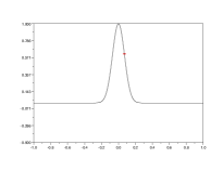
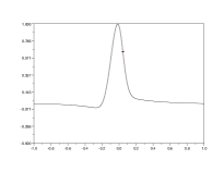
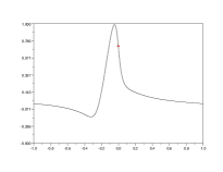
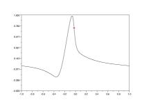
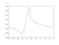
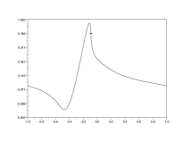
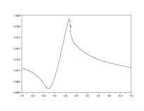
Figure 1. A plunging breaker for the Camassa-Holm equation (17)

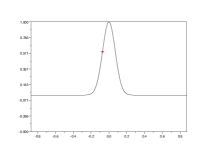
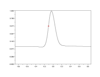
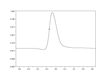
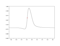
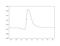
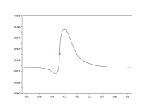
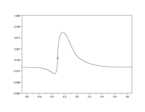
Figure 2. A surging breaker for the surface equation (19)

References

• [1] S. Alinhac, P. Gérard, Opérateurs pseudo-différentiels et thèoréme de Nash-Moser, Savoirs Actuels. InterEditions, Paris; Editions du Centre National de la Recherche Scientifique (CNRS), Meudon, 1991. 190 pp.
• [2] J. Angulo, J. L. Bona, F. Linares, and M. Scialom, Scaling, stability and singularities for nonlinear, dispersive wave equations: the critical case, Nonlinearity 15 (2002), 759–786.
• [3] B. Alvarez-Samaniego, D. Lannes, Large time existence for $3D$ water-waves and asymptotics, preprint.
• [4] B. Alvarez-Samaniego, D. Lannes, A Nash-Moser theorem for singular evolution equations. Application to the Serre and Green-Naghdi equations. Indiana Univ. Math. J., to appear.
• [5] T. B. Benjamin, J. L. Bona and J. J. Mahoney, Model equations for long waves in nonlinear dispersive systems, Phil. Trans. Roy. Soc. London A 227 (1972), 47–78.
• [6] A. Bressan and A. Constantin, Global conservative solutions of the Camassa-Holm equation, Arch. Rat. Mech. Anal. 183 (2007), 215–239.
• [7] R. Camassa and D. Holm, An integrable shallow water equation with peaked solitons, Phys. Rev. Lett. 71 (1993), 1661–1664.
• [8] A. Constantin, On the scattering problem for the Camassa-Holm equation, Proc. Roy. Soc. London A 457 (2001), 953–970.
• [9] A. Constantin and J. Escher, Wave breaking for nonlinear nonlocal shallow water equations, Acta Mathematica 181 (1998), 229–243.
• [10] A. Constantin, V. S. Gerdjikov and R. I. Ivanov, Inverse scattering transform for the Camassa-Holm equation, Inverse Problems 22 (2006), 2197–2207.
• [11] A. Constantin and W. Strauss, Stability of the Camassa-Holm solitons, J. Nonlinear Sci. 12 (2002), 415–422.
• [12] A. D. D. Craik, The origins of water wave theory, Ann. Rev. Fluid Mech. 36 (2004), 1–28.
• [13] A. Degasperis, D. Holm and A. Hone, A new integrable equation with peakon solutions, Theor. Math. Phys. 133 (2002), 1461–1472.
• [14] A. Degasperis and M. Procesi, Asymptotic integrability, in Symmetry and perturbation theory (ed. A. Degasperis $\&$ G. Gaeta), pp 23–37, World Scientific, Singapore, 1999.
• [15] P. G. Drazin and R. S. Johnson, Solitons: an introduction, Cambridge University Press, Cambridge, 1992.
• [16] J. Escher, Y. Liu and Z. Yin, Global weak solutions and blow-up structure for the Degasperis-Procesi equation, J. Funct. Anal. 241 (2006), 457–485.
• [17] A. S. Fokas and B. Fuchssteiner, Symplectic structures, their Bäcklund transformation and hereditary symmetries, Physica D 4 (1981), 821–831.
• [18] B. Fornberg abd G. B. Whitham, A numerical and theoretical study of certain nonlinear wave phenomena, Phil. Trans. Roy. Soc. London A 289 (1978), 373–404.
• [19] A. E. Green and P. M. Naghdi, A derivation of equations for wave propagation in water of variable depth, J. Fluid Mech. 78 (1976), 237–246.
• [20] R. I. Ivanov, On the integrability of a class of nonlinear dispersive wave equations, J. Nonlinear Math. Phys. 12 (2005), 462–468.
• [21] R. S. Johnson, A modern introduction to the mathematical theory of water waves, Cambridge University Press, Cambridge, 1997.
• [22] R. S. Johnson, Camassa-Holm, Korteweg-de Vries and related models for water waves, J. Fluid Mech. 457 (2002), 63–82.
• [23] D. J. Korteweg and G. de Vries, On the change of form of long waves advancing in a rectangular canal and on a new type of long stationary waves, Phil. Mag. 39 (1895), p. 422.
• [24] J. Lenells, Conservation laws of the Camassa-Holm equation, J. Phys. A 38 (2005), 869–880.
• [25] Y. A. Li, A shallow-water approximation to the full water wave problem, Commun. Pure Appl. Math. 59 (2006), 1225–1285.
• [26] Y. Matsuno, The $N$-soliton solution of the Degasperis-Procesi equation, Inverse Problems 21 (2005), 2085–2101.
• [27] H. P. McKean, Breakdown of the Camassa-Holm equation, Comm. Pure Appl. Math. 57 (2004), 416–418.
• [28] L. Molinet, On well-posedness results for the Camassa-Holm equation on the line: a survey, J. Nonlin. Math. Phys. 11 (2004), 521–533.
• [29] D. H. Peregrine, Calculations of the development of an undular bore, J. Fluid Mech. 25 (1966), 321–330.
• [30] P. E. Souganidis and W. A. Strauss, Instability of a class of dispersive solitary waves, Proc. Roy. Soc. Edinburgh Sect. A 114 (1990), 195–212.
• [31] J. J. Stoker,1957 Water waves, New York: Interscience Publ., Inc., 1957.
• [32] T. Tao, Low-regularity global solutions to nonlinear dispersive equations, in Surveys in Analysis and Operator Theory, Proc. Centre Math. Appl. Austral. Nat. Univ., 19–48, 2002.
• [33] G. B. Whitham, Linear and nonlinear waves, J. Wiley & Sons, New York, 1974.