Stellar Photon and Blazar Archaeology with Gamma-rays

Abstract

Ongoing deep surveys of galaxy luminosity distribution functions, spectral energy distributions and backwards evolution models of star formation rates can be used to calculate the past history of intergalactic photon densities and, from them, the present and past optical depth of the universe to $\gamma$-rays from pair production interactions with these photons. Stecker, Malkan & Scully have recently calculated the densities of intergalactic background light (IBL) photons of energies from 0.03 eV to the Lyman limit at 13.6 eV and for redshifts 0$<z<$ 6, using deep survey galaxy observations from the Spitzer, Hubble and GALEX space telescopes. From these results, they have predicted absorption features for blazar spectra.

This proceedure can also be reversed by looking for sharp cutoffs in the spectra of extragalactic $\gamma$-ray sources at high redshifts in the multi-GeV energy range with GLAST (the Gamma-ray Large Area Space Telescope). Determining the cutoff energies of sources with known redshifts and little intrinsic absorption may enable a more precise determination of the IBL photon densities in the past, i.e., the ”archaeo-IBL”, and therefore allow a better measure of the past history of the total star formation rate, including that from galaxies too faint to be observed.

Conversely, observations of sharp high energy cutoffs in the $\gamma$-ray spectra of blazars at unknown redshifts can be used instead of spectral lines to give a measure of their redshifts. Also, given a knowledge of the archaeo-IBL, one can derive the intrinsic $\gamma$-ray spectra and luminosities of blazars over a range of redshifts and look for possible trends in blazar evolution. Stecker, Baring & Summerlin have found some evidence hinting that TeV blazars with flatter spectra have higher intrinsic TeV $\gamma$-ray luminosities and indicating that there may be a correlation of flatness and luminosity with redshift. GLAST will observe and investigate many blazars in the GeV energy range and will therefore provide much new information regarding this possibility.

1 Introduction

Space-based telescopes that are dedicated to exploring the Universe out to large distances in wavelength ranges from the far-infrared to the X-ray range are now in place and the Gamma-ray Large Area Space Telescope, GLAST, is scheduled to be early next year. These facilities are capable of probing the Universe to study the early primordial phases of star formation and galaxy evolution. Studies of cosmic photons from NASA space observatories supply important inputs as well into astrophysics, physics and cosmology. Presently, the Spitzer space infrared telescope facility is probing deeply into the past to study galaxy formation and evolution in the infrared. GALEX is making similar observational studies in the ultraviolet. In the $\gamma$-ray energy range SWIFT is gathering important information on $\gamma$-ray bursts back to the distant past and GLAST will study sources and diffuse fluxes of $\gamma$-rays at energies up to 100 GeV. The astronomical era of the “deep fields” has arrived.

Whereas archaeological sites such as Chi-chen Itza, which many of us visited on the conference excursion, allow us to peer back to $\sim$kyr in the past, the deep astronomical surveys from the radio to the $\gamma$-ray wavelengths allow us to peer back $\sim$Gyr or more into the history of the Universe.

2 Calculating Intergalactic Archaeophoton Densities

Stecker, Malkan & Scully  [1] have used the approach pioneered in Refs. [2] and  [3] to calculate past intergalactic infrared photon fluxes and densities as they evolved along with the galaxies that produced them. This method, a ”backwards evolution” scheme, is an empirically based calculation which uses as input (1) the luminosity dependent galaxy spectral energy distributions (SEDs) based on observations of normal galaxy infrared SEDs, (2) observationally based galaxy luminosity distribution functions (LFs) and (3) redshift dependent galaxy luminosity evolution functions. These are empirically derived curves giving the universal star formation rate or luminosity density as a function of redshift, which are referred to as Lilly-Madau plots. Ref. [1] uses new deep survey observations, primarily from the Spitzer infrared space observatory, to make improvements to the previous calculations of Refs. [2] and  [3].

Figure 1: Empirically derived galaxy SEDs for various luminosities from $10^{-3}L_{*}$ to $10{{}^{3}}L_{*}$.

2.1 Galaxy Infrared SEDs as a Function of Luminosity

The key empirically supported assumption made in Ref. [1] is that the luminosity of a galaxy determines the average galaxy SED and that therefore the galaxy luminosity distribution function (LF) can be predicted statistically from its observed luminosity in one infrared waveband, here chosen to be 60$\mu$m [4]. It is a well-established fact that more luminous galaxies (now and in the past) have higher rates of ongoing star formation and that the star formation rate was higher in the past.

Empirically, it is also found that for the more luminous galaxies, relatively more of the energy from these young stars is absorbed by dust grains and re-radiated in the thermal infrared; more luminous galaxies have higher infrared flux relative to optical flux and warmer infrared spectra. These clear luminosity-dependent trends in galaxy SEDs were well determined locally from the combination of IRAS (Infrared Astronomy Satellite) and ground-based photometry for large (e.g., all sky) samples. The infrared SEDs as a function of galaxy luminosity used in [1] were based on broadband photometry of IRAS selected samples and show the average SED emission trends discussed above. The family of average galaxy SEDs at various luminosities in terms of $L_{*}$ is shown in Figure 1, taken from Ref. [2], where $L_{*}=8.4\times 10^{23}$ W Hz^-1 is the luminosity at 60 $\mu$m.

Other computations of infrared backgrounds and source counts have used different SEDs, based on somehwat different combinations of data and models, in some cases estimated in more spectral detail. One may ask whether these new SEDs might differ from those used in Refs. [2], [3] and [1], either in overall colors, or in detail around the 7–12$\mu$m region, where the strongest spectral features from polycyclic aromatic hydrocarbon (PAH) emission and silicate emission are found. The best example of these new galaxy template SEDs can be found in Ref [5]. As shown in Ref. [1], the agreement between the infrared SEDs in Refs. [5] and  [1] is excellent. As long as this agreement holds for SEDs of galaxies near the “knee” of the approximate broken power-law LFs is reasonable (see Figure 2), the final computed intergalactic photon densities will also agree, because they are dominated by galaxies with luminosities $\sim L_{*}$ around the knee.

2.2 The Local Infrared Luminosity Function

The foundation of the backwards evolution calculation [1] is an accurately determined local infrared luminosity function of galaxies. We used the LF observationally derived in Ref. [4] because it was based on an extensive analysis of very large data sample of galaxies. This LF was updated by using the even more thorough local infrared LF given in the more recent Ref. [6]. A low-luminosity power-law index of -1.35 was adopted in Ref. [1] for the broken power-law differential LF which steepened by 2.25 at high luminosities. This LF takes better account of the large number of fainter galaxies that are now known [7]. The cosmological values adopted in Ref.  [1] were $h=0.7$ and a $\Lambda$CDM cosmology with $\Omega_{\Lambda}=0.7$ and $\Omega_{m}=0.3$.

Figure 2: 60$\mu$m local galaxy luminosity function.

Figure 2 compares the broken power-law LF at $z=0$ with the data given in Ref. [6]. Note that the luminosity $L_{*}$ used in Figure  1 is defined to be the luminosity at the knee of the LF shown in Figure  2. It can be seen that the agreement between the analytic curve and the observational data is excellent.

2.3 Evolution of the IBL SED with Redshift

It is now well known that galaxies had a brighter past owing to their higher rates of star formation and the fading of stellar populations as they age. The simplest resulting evolution of the galaxy luminosity function is a uniform shift in either the vertical axis (number density evolution), or in the horizontal axis (luminosity evolution.) For a pure power-law luminosity function, number and luminosity evolution are mathematically equivalent. In reality, however, to avoid unphysical divergences in the total number or luminosity of galaxies, the luminosity function must steepen at high L and flatten at low L. Thus real LF’s will have at least one characteristic “knee” separating the steep high-L portion from the flatter low-L slope. For typical LF’s this results in most of the luminosity being emitted by galaxies within an order of magnitude of this knee. Thus large uncertainties and errors in the LF far from this knee will hardly change most of the results (e.g., number counts and integrated diffuse backgrounds).

Strong luminosity evolution of galaxies, i.e., a substantial increase in the luminosity of this knee with redshift, is consistently found by many observations relating infrared luminosity to the much higher star formation rate at $z\sim 1$ and to the recent determination that most ultraviolet-selected galaxies at $z\sim 1$ are also luminous infrared galaxies.

The exact form of the luminosity evolution of galaxies is the most uncertain input to the calculation of the IBL density, since it depends on high redshift data. Therefore, two plausible cases of pure luminosity evolution were adopted in Ref. [1] in order to bracket the uncertainties from the deep surveys: (1) a more conservative “baseline” (B) evolution scenario and (2) a “fast evolution” (FE) scenario. A more detailed discussion of these models is given in Ref. [1]. The FE model is favored by recent Spitzer observations [8, 9]. It also provides a better description of the deep Spitzer number counts at 70 and 160$\mu$m than the B model. However, GALEX (Galaxy Evolution Explorer) observations indicate that the redshift evolution of ultraviolet radiation may be more consistent with the B model [10]. The Spitzer IRAC (Infrared Array Camera) counts can be best fit with an evolution rate between these two models. One way of understanding the somewhat smaller redshift evolution of the star formation rate implied by the GALEX ultraviolet observations vs. that obtained from the Spitzer infrared observations is that the effect of dust extinction followed by infrared reradiation increases with redshift [11].

3 Calculation of the Intergalactic Background Light

Our calculation of the diffuse infrared background as described above extends up to a rest frequency of $\log\nu_{Hz}=14.1.$ corresponding to an energy of $\sim 0.5$ eV. This is the location of the peak in the spectral energy distributions of most galaxies and is produced by the light of red giant stars. The spectrum (in energy density units) then curves downward rapidly to higher frequencies, with modest dependence on galaxy luminosity. Although galaxy SEDs have a peak at this energy, this peak, as opposed to the far infrared peak in galaxy SEDs, only manifests itself as an inflection point in the photon density spectrum. At wavelengths shortward of this near infrared-optical “peak’ the photon density spectra drop steeply (See Figures 3 and 4 which plot $\epsilon n(\epsilon)$ for the case of the fast evolution (FE) model.) The relative increase in the ratio of red-to-blue photons at the higher redshifts shown in these figures is produced by early generation, low luminosity stars.

The low redshift extragalactic background light (EBL) SEDs obtained are shown in Figure  5. They are given for the two evolution models previously discussed, viz., the “baseline” (B) model and the “fast evolution” (FE) model.

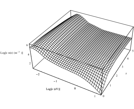
Figure 3: The photon density $\epsilon n(\epsilon)$ shown as a continuous function of energy and redshift.

Figure 4: The photon density $\epsilon n(\epsilon)$ function of energy for various redshifts based on the fast evolution model for infrared evolution. The solid line is for $z=0$, the dashed line is for $z=1$ , the dotted line is for $z=3$, the dot-dashed line is for $z=5$.

Figure 5: Spectral energy distribution of the diffuse background radiation at $z=0$, sometimes referred to as the extragalactic background light (EBL). Error bars show data points, triangles show lower limits from number counts, and the inverted triangle shows an upper limit from TeV observations  [12]. The upper and lower solid lines show the fast evolution and baseline evolution predictions, and the dotted lines show their extensions into the optical–ultraviolet, as described in Ref. [13].

4 Gamma-ray Absorption from Pair Production Interactions

The potential importance of the photon-photon pair production process, $\gamma\gamma\rightarrow e^{+}e^{-}$, in high energy astrophysics has been realized for over 40 years [14]. It was pointed out that owing to interactions with the 2.7 K CMB, the universe would be opaque to $\gamma$-rays of energy above 100 TeV at extragalactic distances [15, 16]. If one considers cosmological and redshift effects, it was further shown that photons from a $\gamma$-ray source at a redshift $z_{s}$ would be significantly absorbed by pair production interactions with the CMB above an energy $\sim 100(1+z_{s})^{-2}$ TeV [17, 18].

Following the discovery by the EGRET team of the strongly flaring $\gamma$-ray blazar 3C279 at redshift 0.54 [19], Stecker, de Jager and Salamon [20] proposed that one can use the predicted pair production absorption features in blazars to determine the intensity of the infrared portion of the IBL, provided that the intrinsic spectra of blazars extends to TeV energies. It was later shown that the IBL produced by stars in galaxies at redshifts out to $\sim 2$ would make the universe opaque to photons above an energy of $\sim 30$ GeV emitted by sources at a redshift of $\sim 2$, again owing to pair production interactions [21, 13].

As discussed above, in Ref. [1] this approach was expanded by using recent data from the Spitzer infrared observatory In addition, data from the Hubble deep survey and the GALEX mission were also used to determine the photon density of the IBL from 0.03 eV to the Lyman limit at 13.6 eV for redshifts out to 6 (the “archaeo-IBL”). The results, giving the IBL photon density as a function of redshift together with the opacity of the CMB as a function of redshift, were then used to calculate the opacity of the universe to $\gamma$-rays for energies from 4 GeV to 100 TeV and for redshifts from $\sim 0$ to 5.

The results of Ref. [1] as shown in Figure 6 imply that the universe will become opaque to $\gamma$-rays for sources at the higher redshifts at somewhat lower $\gamma$-ray energies than those given in Ref. [13]. This dependence is shown in Figure 8. The increased opacity calculated at the higher redshifts is because the newer deep surveys have shown that there is significant star formation out to redshifts $z\geq 6$ [25, 26]), greater than the value of $z_{max}=4$ assumed in Ref. [13]. This conclusion is also supported by recent Swift observations of the redshift distribution of GRBs [27].

Figure 6: Optical depth of the universe to $\gamma$-rays from interactions with photons from the EBL and 2.7K CMB for various redshifts, $z$. The solid lines are for the FE model and the dashed lines are for the B model. The curves shown are for (from top to bottom) $z$ = 5.0, 3.0, 2.0, 1.0, 0.5, 0.2, 0.117, 0.03[1].

Table 1. Optical Depth Parameters for the Fast Evolution and Baseline Models Evolution Model A B C D Fast Evolution -0.475 21.6 -0.0972 10.6 Baseline -0.346 16.3 -0.0675 7.99

Stecker, Malkan and Scully [1] found that the function $\tau(E_{\gamma},z)$ shown in Figure  6 can be very well approximated by the analytic form

$$\log\tau=Ax^{4}+Bx^{3}+Cx^{2}+Dx+E$$ (1)

over the range $0.01<\tau<100$ where $x\equiv\log E_{\gamma}$ (eV). The correct coefficients A through E are given for various redshifts in Ref. [28]. (This is the corrected form of the original table given in Ref. [1].)

5 Photon Archaeology

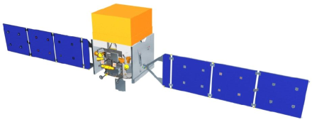
Figure 7: Schematic of the GLAST satellite deployed in orbit. The LAT, which comprises of a cluster of 16 silicon strip trackers and a calorimeter consisting of 8 layers of CsI(Tl) crystals, is in the top (yellow) area; the Gamma Ray Bust Monitors GBM are located directly below.

Observations of relatively nearby blazars using the H.E.S.S. and MAGIC air Čerenkov telescopes have produced many results in the TeV energy range. However, as can be seen from Figure  6, the critical energy range for exploring sharp absorption cutoffs from distant blazars is the multi-GeV range. This is an energy range which the upcoming GLAST mission will explore. The GLAST satellite (see Figure  7) will have a large area telescope called the LAT which is designed to study cosmic diffuse $\gamma$-rays and $\gamma$-ray sources in the energy range between $\sim$20 MeV and $>300$ GeV (For more information about GLAST, go to http://glast.stanford.edu/. By using GLAST observations to determine the absorption cutoff energies of sources with known redshifts caused by interactions of GeV range $\gamma$-rays with low energy photons of the IBL, we can refine our knowledge of the IBL photon densities in the past, i.e., the archaeo-IBL, and therefore get a better measure of the past history of the total star formation rate. Conversely, observations of sharp high energy cutoffs in the $\gamma$-ray spectra of sources at unknown redshifts can be used instead of spectral lines to give a measure of their redshifts. GLAST must also investigate the possibility that intrinsic absorption within some high luminosity, high redshift $\gamma$-ray sources may mimic absorption by the IBL  [29]. If this is the case, such an effect will need to be disentangled from IBL absorption. One key question is how far the region of $\gamma$-ray emission is from the radiation field surrounding the black hole. There evidence in the case of M87 that the $\gamma$-ray emission region is greater than 120 pc from the black hole [30] arguing against intrinsic absorption. However, this is only one source and it is not a typical blazar. Observationally, intrinsic absorption in active galactic nuclei can be investigated by determining the lower limit envelope on the total absorption from a set of sources in a known narrow redshift range. This can be accomplished by GLAST.

Figure 8: A Fazio-Stecker plot (named after the paper by Fazio & Stecker [18]) which gives the critical optical depth $\tau=1$ as a function of $\gamma$-ray energy and redshift for the fast evolution (solid curve) and baseline (dashed curve) IGL cases. Areas to the right and above these curves correspond to the region where the universe is optically thick to $\gamma$-rays (from Ref. [1].)

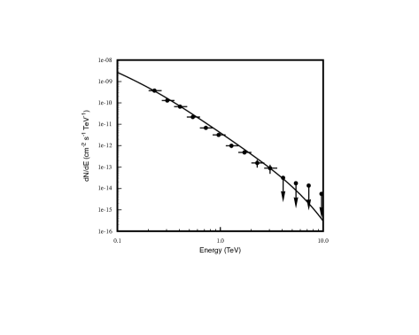
Figure 9: The $\gamma$-ray data from the H.E.S.S. for PKS2155-304 compared with the theoretically obtained spectrum for PKS2155-304 calculated by assuming an intrinsic source spectrum proportional to $E^{-2}$ and multiplying by $e^{-\tau}$ using $\tau(z=0.117)$ for the FE model of Ref. [1].

6 Blazar Spectra and Luminosities, Now and Then

As an example of the application of the $\gamma$-ray absorption models derived in Ref. [1], Figure 9 shows the absorbed spectrum of the blazar PKS 2155-304 at $z=0.117$ assuming that its intrinsic spectrum in the energy range shown is an approximate $E^{-2}$ power law. This spectrum is then compared it with the spectrum observed by the H.E.S.S. TeV $\gamma$-ray telescope array. Thus, one would conclude that the intrinsic (unabsorbed) photon spectrum of this source in the energy range shown has an approximate $E^{-2}$ form.

The intergalactic $\gamma$-ray absorption coefficient (i.e. optical depth), $\tau(E,z)$, increases monotonically with energy and therefore leads to a steepening of the intrinsic source spectra as it is observed at Earth. For sources at redshifts between 0.05 and 0.4, Stecker & Scully  [31] have shown that this steepening results in a well-defined increase in the spectral index of a source with an approximate power-law spectrum in the 0.2 – 2 TeV energy range. This increase is a linear function in redshift $z$ of the form $\Delta\Gamma=C+Dz$, where the parameters $C$ and $D$ are constants. The overall normalization of the source spectrum is also reduced by an amount equal to $exp\{-(A+Bz)\}$ , again where $A$ and $B$ are constants. The values of $A,B,C,$ and $D$ are given for the B and FE models in Table 1.

These analytic relations can be to calculate the intrinsic 0.2 – 2 TeV power-law $\gamma$-ray spectra of sources having known redshifts in the 0.05 – 0.4 range and observed spectral indeces, $\Gamma_{o}$ for both the B and FE models of EBL evolution Table 2, taken from Ref. [32], gives values for $\Gamma_{s}$ for various blazars obtained using the formula given in Ref.  [31]. Table 1 also shows the respective indices $\Gamma_{e}=2\Gamma_{s}-1$ of the electron distributions in the sources under the assumption that the $\gamma$-rays are produced by inverse Compton interactions in the Thomson regime.

Stecker, Baring & Summerlin [32] have also estimated the intrinsic “isotropic luminosity.” of these blazars, also shown in Table 2 The isotropic luminosity of the blazar sources listed in Table 2 is obtained from the formula

$${\cal{L}}\simeq 4\pi{{\Gamma_{o}-2}\over{\Gamma_{s}-2}}(1+z)^{\Gamma_{s}-2}F_{o}[d(z)]^{2}e^{(A+Bz)}$$ (2)

where $d$ is the luminosity distance to the source, and $F_{o}$ is its observed differential energy flux at 1 TeV, and the other factors in the equation give the k-correction for the deabsorbed source spectrum and the normalization correction factor for absorption, $exp\{-(A+Bz)\}$ given in Ref. [31]. The blazars Mrk 421 and Mrk 501 are not included because their redshifts are significantly less than 0.05. However, these blazars are analysed in Ref. [33].

The numbers given in the last column of Table 2 are derived for the fast evolution (FE) model. One may note that there appears to be a trend toward blazars having flatter intrinsic TeV spectra and higher isotropic luminosities at higher redshifts. However, one must be careful of selection effects. The TeV photon fluxes of these sources as observed by H.E.S.S. and MAGIC only cover a dynamic range of a factor of $\sim$20. Therefore, only brighter sources can be observed at higher redshifts. This is because of both diminution of flux with distance and intergalactic absorption [20]. The observed luminosity-redshift trend is naturally expected in a limited population sample spanning a range of redshifts if the TeV-band fluxes are pegged near an instrumental sensitivity threshold. A more powerful handle on the intrinsic spectra and luminosities of these sources will be afforded by the upcoming GLAST $\gamma$-ray mission, with its capability for detecting many blazars at energies below 200 GeV.

Table 2 indicates that some blazars, particularly those observable at the higher redshifts, appear to have very hard intrinsic $\gamma$-ray spectra with indeces in the range between $\sim$1 and $\sim$1.5. The possibility that such spectra can be obtained from shock acceleration has not usually been admitted when considering properties of blazar jets and their possible emission spectra [34]. However, such spectra can be produced by relativistic shock acceleration [32], as discussed in the next section. We will also discuss observational evidence in the hard X-ray range for $\gamma$-ray blazars with spectral indeces in the range between $\sim$1 and $\sim$1.5.

Table 2. Blazar Spectral Indeces in the 0.2-2 TeV Energy Range and TeV Luminosities Source Name $z$ $\Gamma_{obs}$ $\Gamma_{source}$(FE $\rightarrow$ B) $\Gamma_{e}$(FE $\rightarrow$ B) $\cal{L}$(1 TeV) [$10^{36}$ W 1ES 2344+514 0.044 3.0 2.5 $\rightarrow$ 2.6 4.0 $\rightarrow$ 4.2 2.9 Mrk 180 0.045 3.3 2.9 $\rightarrow$ 3.0 4.8 $\rightarrow$ 5.0 1.2 1ES1959+650 0.047 2.7 2.3 $\rightarrow$ 2.4 3.6 $\rightarrow$ 3.8 5.4 PKS 2005-489 0.071 4.0 3.4 $\rightarrow$ 3.5 5.8 $\rightarrow$ 6.0 8.6 PKS 2155-304 0.117 3.3 2.2 $\rightarrow$ 2.4 3.4 $\rightarrow$ 3.8 420 H 2356-309 0.165 3.1 1.5 $\rightarrow$ 1.9 2.0 $\rightarrow$ 2.8 200 1ES 1218+30 0.182 3.0 1.2 $\rightarrow$ 1.6 1.4 $\rightarrow$ 2.2 310 1ES 1101-232 0.186 2.9 1.0 $\rightarrow$ 1.5 1.0 $\rightarrow$ 2.0 230 1ES 0347-121 0.188 3.1 1.2 $\rightarrow$ 1.7 1.4 $\rightarrow$ 2.4 1200 1ES 1101+496 0.212 4.0 1.8 $\rightarrow$ 2.4 2.6 $\rightarrow$ 3.8 930

7 Shock Acceleration and Intrinsic Blazar Spectra

The rapid variability seen in TeV flares drives the prevailing picture for the blazar source environment, one of a compact, relativistic jet that is structured on small spatial scales that are unresolvable by present $\gamma$-ray telescopes. Turbulence in the supersonic outflow in these jets naturally generates relativistic shocks, and these form the principal sites for acceleration of electrons and ions to the ultrarelativistic energies implied by the TeV $\gamma$-ray observations. Within the context of this relativistic, diffusive shock acceleration mechanism, numerical simulations can be used to derive expectations for the energy distributions of particles accelerated in blazar jets.

Diffusive acceleration at relativistic shocks is less well studied than for nonrelativistic flows, yet it is the most applicable process for extreme objects such as pulsar winds, jets in active galactic nuclei, and $\gamma$-ray bursts. A key characteristic that distinguishes relativistic shocks from their non-relativistic counterparts is their inherent anisotropy due to rapid convection of particles through and away downstream of the shock. This renders analytic approaches more difficult for ultrarelativistic upstream flows, though advances can be made in special cases, such as the limit of extremely small angle scattering (pitch angle diffusion). Accordingly, complementary Monte Carlo techniques have been employed for relativistic shocks in a number of studies, including test-particle analyses for steady-state shocks of parallel and oblique magnetic fields (see refs. in Ref.  [32]). This approach was used in Ref. [32] to determine key spectral characteristics for particles accelerated to high energies at relativistic shocks that are of relevance to acceleration in blazar jets. For a discussion of relativistic shock acceleration, see Ref. [35].

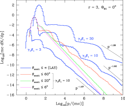
Figure 10: Particle distribution functions $dN/dp$ from parallel relativistic shocks obtained from a Monte Carlo simulation of particle diffusion and gyrational transport. Scattering off hydromagnetic turbulence is modeled by randomly deflecting particle momenta by an angle within a cone, of half-angle $\theta_{scatt}$, whose axis coincides with the particle momentum prior to scattering. The thick (blue) lines are for the large angle scattering cases (LAS). These asymptotically approach the power-laws indicated by thin lines, at high and very high energies (not shown). Three smaller angle scattering cases are also shown, corresponding to pitch angle diffusion (PAD). These have high-energy asymptotic power-law indices of 1.65, 1.99 and 2.20.

Representative particle momentum distributions that result from the simulation of diffusive acceleration at relativistic shocks are depicted in Figure 10 [32]. These distributions are equally applicable to electrons or ions, and so the mass scale is not specified. These results highlight several key features. The momentum distributions are flatter when produced by faster shocks with a larger upstream flow bulk Lorentz factor of the jet, $\gamma_{1}$, given a fixed velocity compression ratio. This is a consequence of the increased kinematic energy boosting occurring at relativistic shocks. Such a characteristic is evident for much larger angle scattering, as found in the work of other authors referenced in Ref. [32]. What is much more striking in Figure 10 is that the slope and shape of the nonthermal particle distribution depends on the nature of the scattering. The asymptotic, ultrarelativistic index of $\Gamma_{e}=2.23$ is realized only in the mathematical limit of small (pitch) angle diffusion (PAD), where the particle momentum is stochastically deflected on arbitrarily small angular (and therefore temporal) scales. In practice, PAD results when the maximum scattering angle $\theta_{scatt}$ is less than the Lorentz cone angle 1/$\gamma_{1}$ in the upstream region. In such cases, particles diffuse in the region upstream of the shock only until their angle to the shock normal exceeds $\sim 1/\gamma_{1}$. Then they are rapidly swept to the downstream side of the shock. The energy gain per shock crossing cycle is then roughly a factor of two, simply derived from relativistic kinematics.

To contrast these power-law cases, Figure 10 also shows the results given in Ref. [32] for large angle scattering scenarios (LAS, with $\theta_{scatt}\sim\pi$), where the spectrum is highly structured and much flatter on average than $p^{-2}$. The structure, which becomes extremely pronounced for large $\gamma_{1}$, is kinematic in origin, where large angle deflections lead to the distribution of fractional energy gains between unity and $\gamma_{1^{2}}$ in successive shock transits by particles. Gains like this are kinematically analogous to the photon energy boosting by inverse Compton scattering. Each structured bump or spectral segment shown in Figure 10 corresponds to an increment in the number of shock crossings, successively from $1\to 3\to 5\to 7$ etc. They eventually smooth out to asympotically approach power-laws that are indicated by the lightweight lines in the Figure. The indices of these asymptotic results are all in the range $\Gamma_{e}<2$. Intermediate cases are also depicted in Figure 10, with $\theta_{scatt}\sim 4/\gamma_{1}$. The spectrum is smooth, like the PAD case, but the index is lower than 2.23. Astrophysically, there is no reason to exclude such cases. From the plasma point of view, magnetic turbulence could easily be sufficient to effect scatterings on this intermediate angular scale, a contention that becomes even more salient for ultrarelativistic shocks with $\gamma_{1}\gg 10$. It is also evident that a range of spectral indices is produced when $\theta_{scatt}$ is of the order of 1/$\gamma_{1}$. In this case, the scattering processes corresponds to a transition between the PAD and LAS limits.

The implications of the numerical simulations given in Ref. [32] for distributions of relativistic particles in blazars are apparent. There can be a large range in the spectral indices $\Gamma_{e}$ of the particles accelerated in relativistic shocks, and these indices usually differ from $\Gamma_{e}\sim 2.23$. They can be much steeper, particularly in oblique shocks. However, they can also be much flatter, so that quasi-power-law particle momentum distributions $p^{-\Gamma_{e}}$ with $\Gamma_{e}\leq 2$ are readily achievable. These spectra can be preserved, provided that the electron spectra produced during blazar flares are not significantly affected by cooling by synchroton radiation. This requires that $t_{acc}<t_{ccol}$ which constrains both the magnetic field strength and the electron energy for gyrorsonant acceleration processes  [36]. These electrons can then Compton scatter to produce $\gamma$-ray spectra with $\Gamma<1.5$.

In fact, recent obsevations of an extreme MeV $\gamma$-ray blazar at a redshift of $\sim$3 by Swift [37] and the powerful $\gamma$-ray quasar PKS 1510-089 at a redshift of 0.361 by Swift and Suzaku  [38] both exhibited power-law spectra in the hard X-ray range which were significantly harder than 1.5, implying electron spectra significantly harder than value of 2 usually considered for shock acceleration. Spectra in the hard X-ray range do not suffer intergalactic absorption so that there is no ambiguity concerning their spectral indeces.

8 Blazar Archaeology

It can be seen from Figure 6 that for $\gamma$-ray sources at the higher redshifts there is a steeper energy dependence of the optical depth $\tau(E_{\gamma})$ near the energy where $\tau=1$. There will thus be a sharper absorption cutoff for sources at high redshifts. It can easily be seen that this effect is caused by the sharp drop in the ultraviolet photon density at the Lyman limit.

It is expected that GLAST will be able to resolve out thousands of blazars from the general extragalactic $\gamma$-ray background [39]. Because of the strong energy dependence of absorption in blazar spectra at the higher redshifts in the multi-GeV range, GLAST will be able to probe the archaeo-IBL and thereby probe the early star formation rate. GLAST should be able to detect blazars at known redshifts $z\sim 2$ at multi-GeV energies and determine their critical cutoff energy. A simple observational technique for probing the archaeo-IBL has been proposed in Ref. [40]. In such ways, GLAST observations at redshifts $z\geq 2$ and $E_{\gamma}\sim 10$ GeV may complement the deep galaxy surveys by probing the total star formation rate, even that from galaxies too faint to be detected in the deep surveys. Future GLAST observations in the 5 to 20 GeV energy range may also help to pin down the amount of dust extinction in high-redshift galaxies by determining the mean density of ultraviolet photons at the higher redshifts through their absorption effect on the $\gamma$-ray spectra of high redshift sources. If the diffuse $\gamma$-ray background radiation is from unresolved blazars [39], a hypothesis which can be independently tested by GLAST [41], absorption will steepen the spectrum of this radiation at $\gamma$-ray energies above $\sim 10$ GeV [13]. Thus, GLAST can also aquire information about the evolution of the IBL in this way.

Conversely, observations of sharp high energy cutoffs in the $\gamma$-ray spectra of sources at unknown redshifts can be used instead of spectral lines to give a measure of their redshifts.

Table 2 indicates that there may be an evolution of TeV blazars with redshift, both in luminosity and spectral index. It may be that past blazars had jets with higher bulk Lorentz factors than low-redshift BL Lacs. It may also be that these apparent trends are only the result of selection effects. There is only a small sample of ten sources listed in Table 2. GLAST will be able to explore this question, as it has the potential of seeing thousands of blazars [39].

9 Extragalactic Astronomy: The Greatest Dig in the Universe

In keeping with the cosmic high energy theme of the 30th International Cosmic Ray Conference, the emphasis in this paper has been on high energy photons ($\gamma$-rays). However, we have seen the intimate connection between these photons and the low energy photons that are the subjects of more traditional astronomy. In fact, radio surveys, ongoing infrared-to-ultraviolet deep astronomical surveys, and surveys of the more newly discovered extragalactic $\gamma$-ray sources and $\gamma$-ray bursts, are most effectively used when considered together to create a consistent and compelling picture of the past history of the Universe.

10 Epilogue

In memory of Frank Culver Jones, my onetime mentor and friend for four decades. Frank passed away earlier this year. He only missed one ICRC conference since 1961. He also served as secretary to the ICRC. He will be missed by the cosmic-ray community.

References

- [1] F. W. Stecker, M. A. Malkan & S. T. Scully, Astrophys. J. 648, 774 (2006).
- [2] M. A. Malkan & F. W. Stecker, F.W., Astrophys. J. 496, 13 (1998).
- [3] M. A. Malkan & F. W. Stecker, Astrophys. J. 555, 641 (2001).
- [4] W. Saunders, et al. , Mon. Not. Roy. Astr. Soc. 242, 318 (1990).
- [5] C. K. Xu, et al. , Astrophys. J. 562, 179 (2001).
- [6] T. T. Takeuchi, K. Yoshikawa, & T. T. Ishii, T.T., Astrophys. J. 587, L89.
- [7] M. R. Blanton, et al. , Astrophys. J. 631, 208 (2005).
- [8] Le Floc’h et al., Astrophys. J. 632, 169 (2005).
- [9] P. G. Pérez-González et al. Astrophys. J. 630, 82 (2005).
- [10] D. Schiminovich et al., Astrophys. J. 619, L47 (2005).
- [11] D. Burgarella et al. (GALEX team), in The Dusty and Molecular Universe, ed. A. Wilson (ESA SP-577); Nordwijk: ESA), 141 (2006).
- [12] F. W. Stecker & O. C. de Jager, in Proc. Kruger Park Intl. Workshop on TeV Gamma Ray Astrophysics, ed. O. C. de Jager (Potchefstoom: Wesprint), 39, e-print astro-ph/9710145.
- [13] M. H.Salamon, & F. W. Stecker, F.W., Astrophys. J. 493, 547 (1998).
- [14] A. I. Nikishov, Sov. Phys. JETP 14, 373 (1962).
- [15] R. J. Gould and G. Schréder, Phys. Rev. Letters 16, 252 (1966).
- [16] J. V. Jelly, Phys. Rev. Letters 16, 479 (1966).
- [17] F. W. Stecker, Astrophys. J. 157, 507 (1969).
- [18] G. G. Fazio and F. W. Stecker, Nature 226, 135 (1970).
- [19] R. C. Hartman et al., Astrophys. J. 385, L1 (1992).
- [20] F. W. Stecker, O. C. De Jager and M. H. Salamon, Astrophys. J. 390, L49 (1992).
- [21] P. Madau and E. S. Phinney, Astrophys. J. 456, 124 (1996).
- [22] T. Totani and T. T. Takeuchi, Astrophys. J. 570, 470 (2002).
- [23] T. M. Kneiske, K. Mannheim and D. H. Hartmann, Astron. and Astrophys. 386, 1 (2002).
- [24] T. M. Kneiske et al., Astron. and Astrophys. 413, 807 (2004).
- [25] A. J. Bunker et al. Mon. Not. Roy. Ast. Soc. 355, 374 (2004).
- [26] R. J. Bouwens et al. Astrophys. J. 653, 53 (2006).
- [27] N. R. Tanvir and P. Jakobson, Phil Trans Roy. Soc. A, in press, e-print astro-ph/0701777.
- [28] F. W. Stecker, M. A. Malkan and S. T. Scully, Astrophys. J. 658, 1392 (2007).
- [29] A. Reimer, Astrophys. J. 665, 1023 (2007).
- [30] C. C. Cheung, D. E. Harris & Ł.Stawarz, Astrophys. J. 663, L65.
- [31] F. W. Stecker & S. T. Scully, Astrophys. J. 652, L9 (2006).
- [32] F. W. Stecker, M. G. Baring & E. J. Summerlin, Astrophys. J., (Letters) 667, L29 (2007).
- [33] A. Konopelko et al. , Astrophys. J. 597, 851 (2003).
- [34] F. Aharonian et al., Nature 440, 1018 (2006).
- [35] M. G. Baring, Nucl. Phys. B, 136C, 198 (2004), e-print astro-ph/0409303.
- [36] M. G. Baring, Publ. Astron. Soc. Australia, 19, 60 (2002).
- [37] R. M. Sambruna et al. , Astrophys. J. 646, 23 (2006).
- [38] J. Kataoka et al. , Astrophys. J. 671, in press, e-print arXiv:0709.1528.
- [39] F. W. Stecker & M. H. Salamon, Astrophys. J. 464, 600. (1996).
- [40] A. Chen, L. C. Reyes & S. Ritz, Astrophys. J. 608, 686 (2004).
- [41] F. W. Stecker & M. H. Salamon, Proc. XXVI Intl. Cosmic Ray Conf. ed. D. Kieda, M. Salamon and B. Dingus 3, 313 (1999); e-print astro-ph/9909157.