On the existence of tight contact structures on Seifert fibered 3–manifolds

Abstract

We determine the closed, oriented Seifert fibered 3–manifolds which carry positive tight contact structures. Our main tool is a new non–vanishing criterion for the contact Ozsváth–Szabó invariant.

57R17 57R57

1 Introduction

Let $Y$ denote a closed, oriented 3–manifold. A smooth 1–form $\alpha\in\Omega^{1}(Y)$ is a positive contact form on $Y$ if $\alpha\wedge d\alpha>0$. The 2–plane field

$$\xi:=\ker\alpha\subset TY$$

is called a (cooriented) positive contact structure. An embedded disk $D^{2}\subset Y$ is an overtwisted disk for $\xi$ if $TD^{2}=\xi$ along $\partial D^{2}$. The contact structure $\xi$ is overtwisted if $Y$ contains an overtwisted disk for $\xi$, otherwise $\xi$ is called tight.

According to [8] every homotopy class of 2–plane fields on a closed, oriented 3–manifold contains a unique up to isotopy overtwisted contact structure, therefore the classification of overtwisted structures reduces to a homotopy theoretic question. Tight contact structures are much harder to find in general. In fact, their existence is not known for a general 3–manifold $Y$, although their presence seems to be related to the geometry of the underlying 3–manifold. Tight contact structures up to isotopy are classified on $S^{3}$, lens spaces [16, 19], circle bundles over surfaces [20] and some special Seifert fibered 3–manifolds [12, 13, 14, 15, 36]. In this paper we address the existence question for tight contact structures on general Seifert fibered 3–manifolds.

Using Legendrian surgery, Gompf [17] showed that each Seifert fibered 3–manifold admits a Stein fillable (hence tight) positive contact structure for at least one choice of orientation. Gompf also conjectured that the Poincaré homology sphere $-P$ with its nonstandard orientation possesses no Stein fillable contact structure. Gompf’s conjecture was verified in [21] using Seiberg–Witten theory, while later Etnyre and Honda [10] showed that $-P$ admits no positive, tight contact structures. This result was extended in [25] to an infinite family $\{M_{n}\}_{n\geq 1}$ of small Seifert fibered 3–manifolds, described in the next paragraph.

Let $T_{2,2n+1}\subset S^{3}$, for each integer $n\geq 1$, denote the $(2,2n+1)$–torus knot, whose planar diagram is illustrated in Figure 1.

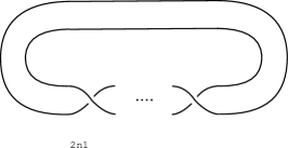
Figure 1: The diagram of the torus knot $T_{2,2n+1}$, $n\geq 1$.

Let $M_{n}$, for each $n\geq 1$, be the 3–manifold obtained by performing $(2n-1)$–surgery along $T_{2,2n+1}$ in $S^{3}$. The 3–manifold $M_{n}$ can be also be viewed as the boundary of the 4–dimensional plumbing prescribed by the weighted tree of Figure 2, where weights equal to $-2$ are omitted. (For the equivalence of the two presentations of $M_{n}$ see [25, Figure 2].)

Figure 2: The plumbing tree describing $M_{n}$

It is well known that $M_{n}$ carries a Seifert fibered structure for each $n\geq 1$, and the manifold $M_{1}$ is diffeomorphic to $-P$ above. The main result of the present paper is

Theorem 1.1.

Let $Y$ be a closed, oriented Seifert fibered 3–manifold. Then, either $Y$ is orientation–preserving diffeomorphic to $M_{n}$ for some $n\geq 1$, or $Y$ carries a positive, tight contact structure.

Since by [25, Corollary 1.2] each 3–manifold $M_{n}$ carries no positive tight contact structures, Theorem 1.1 yields a complete solution to the existence problem for positive tight contact structures on Seifert fibered 3–manifolds.

The paper is organized as follows. In Section 2 we collect the results about tight contact structures on Seifert fibered 3–manifolds known before Heegaard Floer theory. In Section 3 we introduce Heegard Floer theory methods and we use them to give a new criterion for the existence of tight contact structures on Seifert fibered 3–manifolds. In Sections 4 and 5 we apply the criterion to prove the existence of tight contact structures for several families of Seifert fibered 3–manifolds. In Section 6 we use the results of Sections 2, 4 and 5 to prove Theorem 1.1.

Acknowledgements: The second author was partially supported by OTKA 49449, by EU Marie Curie TOK program BudAlgGeo and by Clay Mathematics Institute.

2 First constraints on the Seifert invariants

In this section we collect several known results on the existence of tight contact structures on Seifert fibered 3–manifolds, summarizing in Proposition 2.2 what was known before Heegard Floer theory. For definitions and basic facts about Seifert fibered 3–manifolds we refer to [34].

Let $f\co Y_{e_{0}}\to S^{2}$ be an oriented three–dimensional circle bundle over the 2–sphere, with Euler number $e_{0}\in\mathbb{Z}$. Let $F_{1},\ldots,F_{k}\subset Y_{e_{0}}$ be $k$ distinct fibers of the map $f$, and denote by $Y(e_{0};r_{1},\ldots,r_{k})$, with $r_{i}\in(0,1)\cap\mathbb{Q}$, the oriented 3–manifold resulting from $(-\frac{1}{r_{i}})$–surgery along $F_{i}$, $i=1,\ldots,k$, with the convention that the $0$–framing on $F_{i}$ is given naturally by the fibration $f$. It is a well–known fact that each manifold $Y(e_{0};r_{1},\ldots,r_{k})$ carries a Seifert fibration over $S^{2}$ with $k$ multiple fibers and, conversely, each oriented Seifert fibered 3–manifold with base $S^{2}$ and $k$ multiple fibers is orientation–preserving diffeomorphic to $Y(e_{0};r_{1},\ldots,r_{k})$ for some $r_{i}\in(0,1)\cap\mathbb{Q}$, $i=1,\ldots,k$ and $e_{0}\in\mathbb{Z}$.

The rational Euler characteristic of $Y(e_{0};r_{1},\ldots,r_{k})$ is, by definition,

$$e(Y(e_{0};r_{1},\ldots,,r_{k})):=e_{0}+r_{1}+\cdots+r_{k}.$$

A simple computation shows that the 3–manifold $Y=Y(e_{0};r_{1},\ldots,r_{k})$ is a rational homology sphere, that is $b_{1}(Y)=0$, if and only if $e(Y)\neq 0$.

Proposition 2.1.

Let $Y$ be a closed, oriented, Seifert fibered 3–manifold. Then, either $Y$ carries a tight contact structure or $Y$ is orientation–preserving diffeomorphic to $Y(-1;r_{1},r_{2},r_{3})$ for some $r_{i}\in(0,1)\cap\mathbb{Q}$, $i=1,2,3$, with $e(Y(-1;r_{1},r_{2},r_{3}))>0$.

Proof.

In [17, Theorem 5.4] the existence of Stein fillable (hence tight) contact structures is proved for a Seifert fibered 3–manifold $Y\to F$ provided either $F\neq S^{2}$ or $Y=Y(e_{0};r_{1},\ldots,r_{k})$ with $e_{0}\neq-1$. Therefore, to prove the proposition it suffices to argue that a Seifert fibered 3–manifold $Y$ orientation–preserving diffeomorphic to $Y(-1;r_{1},\ldots,r_{k})$ for some $r_{i}\in(0,1)\cap\mathbb{Q}$, $i=1,2,3$, carries a tight contact structure provided either $k\neq 3$ or $e(Y(-1;r_{1},\ldots,r_{k}))\leq 0$. If the number of multiple fibers $k\leq 2$ then $Y$ is a lens space, which is well–known to carry tight contact structures [16]. If $k\geq 4$ then $Y$ contains incompressible tori and therefore it admits infinitely many distinct tight structures by [2]. If $e(Y)=0$ then $Y$ admits a smooth foliation $\mathcal{F}$ transverse to the Seifert fibration [7]. Moreover, since the fibration has $3$ multiple fibers we have $Y\not\cong S^{2}\times S^{1}$. Therefore $\mathcal{F}$ is a taut foliation and by [9, Theorem 2.4.1 and Corollary 3.2.8] it can be approximated by tight contact structures. Finally, if $e(Y)<0$ then $Y$ is the link of an isolated surface singularity with $\mathbb{C}^{*}$–action [27, Corollary 5.3], and as such it is known to carry tight contact structures (see e.g. [3]). ∎

Proposition 2.2 below shows that for many of the manifolds $Y(-1;r_{1},r_{2},r_{3})$ with $e(Y)>0$ the conclusion of Theorem 1.1 holds. In order to state the proposition we need some preparation which will be useful also later on. Let

$$Y=Y(-1;r_{1},r_{2},r_{3}),\quad r_{1},r_{2},r_{3}\in(0,1)\cap\mathbb{Q},$$

be a small Seifert fibered 3–manifold with $e_{0}(Y)=-1$. From now on we will assume that $r_{1}\geq r_{2}\geq r_{3}$, and that there are continued fraction expansions

$$\frac{1}{r_{1}}=[a_{1},\ldots,a_{n_{1}}],\quad\frac{1}{r_{2}}=[b_{1},\ldots,b_{n_{2}}],\quad\frac{1}{r_{3}}=[c_{1},\ldots,c_{n_{3}}],$$ (2.1)

for some integers $a_{i},b_{j},c_{k}\geq 2$, where, by definition,

$$[x_{1},\ldots,x_{n}]:=x_{1}-\cfrac{1}{x_{2}-\cfrac{1}{\ddots-\cfrac{1}{x_{n}}}}.$$

Expansions (2.1) determine a plumbing tree $\Gamma$ as in Figure 3 and hence, as the result of the corresponding plumbing construction, an oriented 4–manifold $W_{\Gamma}$ with $\partial W_{\Gamma}=Y$. It is not hard to show that $b_{2}^{+}(W_{\Gamma})=1$ if and only if $e(Y)>0$ [27]. As indicated in Figure 3, we will denote by $L_{i}$, for $i=1,2,3$, the leg of the weighted tree $\Gamma$ corresponding to $r_{i}$. More precisely, $L_{1}$ will denote the set of vertices of $\Gamma$ with weights $-a_{1},\ldots,-a_{n_{1}}$, and analogously for $L_{2}$ and $L_{3}$. Moreover, we will denote by $l(L_{i})$, $i=1,2,3$, the length of $L_{i}$, that is its cardinality.

Figure 3:  The plumbing tree $\Gamma$ associated with $Y(-1;r_{1},r_{2},r_{3})$

Similarly, we have

$$-Y(-1;r_{1},r_{2},r_{3})=Y(-2;1-r_{1},1-r_{2},1-r_{3})=\partial W_{\Gamma^{\prime}},$$

where $\Gamma^{\prime}$ is the weighted tree “dual” to $\Gamma$, determined by the continued fraction expansions of $\frac{1}{1-r_{i}}$, $i=1,2,3$. A useful formulation of the relationship between the continued fraction expansions of $\frac{1}{r}$ and $\frac{1}{1-r}$ is given by Riemenschneider’s point rule [35]. The dual tree $\Gamma^{\prime}$ is illustrated in Figure 4.

Figure 4:  The “dual” tree $\Gamma^{\prime}$ associated with $-Y(-1;r_{1},r_{2},r_{3})$

The proof of Proposition 2.2 requires the use of contact surgery [4, 5, 6], so we briefly recall the necessary notions. Suppose that $L\subset(Y,\xi)$ is a Legendrian knot in a contact 3–manifold. The contact structure equips $L$ with a framing (that is, a trivialization of its normal bundle) called the contact framing of $L$. Let $Y_{L}^{\pm}$ denote the 3–manifold obtained by $(\pm 1)$–surgery along $L$, where the surgery coefficient is measured with respect to the contact framing of $L$. According to the classification of tight contact structures on a solid torus [19], the restriction of $\xi$ to the complement of a standard neighborhood of $L$ extends uniquely, up to isotopy, to the surgered manifolds $Y_{L}^{+}$ and $Y_{L}^{-}$, restricting as a tight structure on the glued–up torus. Therefore, the knot $L$ decorated with a $(+1)$ or $(-1)$ uniquely specifies a contact 3–manifold $(Y_{L}^{+},\xi_{L}^{+})$ or $(Y_{L}^{-},\xi_{L}^{-})$. By [8, 17] any contact $(-1)$–surgery along a link in the standard contact 3–sphere produces a Stein fillable, hence tight contact structure. The notion of contact $(\pm 1)$–surgery can be extended to any nonzero rational surgery along a Legendrian knot. The extension of the contact structure is unique, however, only for surgery coefficients of the form $\frac{1}{k}$, with $k\in{\mathbb{Z}}$. In [5, 6] it is shown that a rational contact surgery can be replaced by a sequence of contact $(\pm 1)$–surgeries. For negative surgeries only $(-1)$–surgeries are needed in the replacement.

Proposition 2.2.

Let $Y$ be an oriented, Seifert fibered 3–manifold which is not orientation–preserving diffeomorphic to $Y(-1;r_{1},r_{2},r_{3})$, with $1>r_{1}\geq r_{2}\geq r_{3}>0$ satisfying (2.1) and each of the following:

• $e(Y(-1;r_{1},r_{2},r_{3}))=-1+r_{1}+r_{2}+r_{3}>0$;

• $a_{1}=\cdots=a_{k}=2$ for some $k\geq 1$ and either

  • $n_{1}=k$ or

  • $n_{1}>k$ and $a_{k+1}>2$;

• $c_{1}\geq b_{1}=k+2$.

Then, $Y$ carries a tight contact structure.

Proof.

By Proposition 2.1 we may assume $Y\cong Y(-1;r_{1},r_{2},r_{3})$, with $e(Y)>0$ for some $1>r_{1}\geq r_{2}\geq r_{3}>0$. Notice that $r_{1}\geq r_{2}\geq r_{3}$ implies $a_{1}\leq b_{1}\leq c_{1}$. We can think of the weighted tree $\Gamma$ of Figure 3 as prescribing an integral surgery diagram for $Y$, with each vertex corresponding to an unknot, and each weight corresponding to a surgery coefficient. In the case $a_{1}\geq 3$ we can “blow down”, in the sense of Kirby calculus, the central $(-1)$–circle to get a surgery diagram of unknots, each with surgery coefficient $\leq-2$. Moreover, it is easy to see that the resulting framed link can be isotoped to Legendrian position so that on each component the required topological surgery can be realized by some negative contact surgery. Therefore, by well–known results [17] in this case $Y$ carries Stein fillable structures. This means that we may assume $a_{1}=\cdots=a_{k}=2$ for some $k\geq 1$, so either $n_{1}=k$ or $n_{1}>k$ and $a_{k+1}>2$.

If $b_{1}\geq k+3$ we can blow down the $k+1$ unknots with framing $(-1)$, corresponding to the central vertex of $\Gamma$ together with the first $k$ vertices of $L_{1}$. The components of the resulting framed link $\mathcal{L}$ are pairwise positively linked, and it is easy to see as before that $\mathcal{L}$ has a Legendrian representative such that each topological surgery can be realized by a negative contact surgery. By [5, 6] and [17] this implies that the 3–manifold $Y$ resulting from the surgery carries Stein fillable structures, so we may assume $b_{1}\leq k+2$.

To conclude the proof it suffices to show that $Y$ carries Stein fillable structures if $b_{1}\leq k+1$. In this case we blow–down $b_{1}$ $(-1)$–circles instead of the available $k+1$. After the blow–down operations, the unknot $U$ corresponding to the first vertex of $L_{2}$ has framing $0$, and the unknot $U^{\prime}$ corresponding to the first vertex of $L_{3}$ has framing $-c_{1}+b_{1}\leq 0$. Moreover, since $b_{1}\geq 2$, $U$ and $U^{\prime}$ link positively at least twice. The result of the $0$–surgery on $U$ can be viewed as $S^{2}\times S^{1}$. Then, due to the linking between $U$ and $U^{\prime}$, the remaining topological surgeries in $S^{2}\times S^{1}$ can be realized by negative contact surgeries on $(S^{2}\times S^{1},\xi_{0})$, where $\xi_{0}$ is the standard Stein fillable contact structure on $S^{2}\times S^{1}$ (see e.g. [14, Section 3] for similar arguments). ∎

Remark 2.3.

Observe that each of the 3–manifolds $M_{n}$ defined in Section 1, known not to admit tight contact structures, falls outside the range of applicability of Proposition 2.2. Thus, we can rephrase Proposition 2.2 by saying that in order to prove Theorem 1.1 it suffices to establish the existence of tight contact structures on each 3–manifold distinct from every $M_{n}$ and associated with a plumbing tree $\Gamma$ as in Figure 5. The proof of this existence result will occupy the rest of the paper. We will need arguments of a fairly delicate nature when compared with those used in the proof of Proposition 2.2. The dual tree $\Gamma^{\prime}$ is shown in Figure 6, where weights $-2$ are omitted. Moreover:

$$a^{\prime}_{1}=\begin{cases}k+1\quad\text{if}\quad n_{1}=k,\\ k+2\quad\text{if}\quad n_{1}>k,\end{cases}\quad\text{and}\quad b^{\prime}_{k+1}\begin{cases}=2\quad\text{if}\qua n_{2}=1,\\ >2\quad\text{if}\quad n_{2}>1.\par\end{cases}$$

Figure 5: The constrained plumbing tree $\Gamma$

Figure 6:  The constrained dual tree $\Gamma^{\prime}$

3 Contact invariants and tight contact structures

In this section we introduce and show how to use the crucial ingredient in the proof of Theorem 1.1: the contact Ozsváth–Szabó invariant. We first recall the basic facts of Heegaard Floer theory and a result from [26], which gives a non–vanishing criterion for the contact Ozsváth–Szabó invariant. Then, after some preparatory material, we state and prove Theorem 3.3, which gives a new method to apply the non–vanishing criterion.

Heegaard Floer theory [28, 29, 30, 33] associates a finitely generated abelian group ${{\widehat{HF}}}(Y,\mathbf{t})$, the Ozsváth–Szabó homology group, to a closed, oriented spin^c $3$–manifold $(Y,\mathbf{t})$. Throughout this paper we will assume that $\mathbb{Z}/2\mathbb{Z}$ coefficients are being used in the complexes defining the $\widehat{HF}$–groups. With this assumption, the groups are actually $\mathbb{Z}/2\mathbb{Z}$–vector spaces. The symbol ${{\widehat{HF}}}(Y)$ will denote the direct sum of ${{\widehat{HF}}}(Y,\mathbf{t})$ for all spin^c structures. A fundamental property of these groups is that on each 3–manifold there are only finitely many spin^c structures with non–trivial Ozsváth–Szabó homology group, hence ${{\widehat{HF}}}(Y)$ is also finitely generated. By [29, Proposition 5.1] a rational homology sphere $Y$ has non–trivial Ozsváth–Szabó homology group ${{\widehat{HF}}}(Y,\mathbf{t})$ for each spin^c structure $\mathbf{t}\in Spin^{c}(Y)$. In particular, for a rational homology 3–sphere $Y$ we have

$$\dim{{\widehat{HF}}}(Y)\geq|Spin^{c}(Y)|=|H_{1}(Y;\mathbb{Z})|.$$

A rational homology 3–sphere $Y$ is called an $L$–space if

$$\dim{{\widehat{HF}}}(Y)=|H_{1}(Y;\mathbb{Z})|.$$

In view of the above nonvanishing result, this property is equivalent to

$${{\widehat{HF}}}(Y,\mathbf{t})=\mathbb{Z}/2\mathbb{Z}\quad\text{for each $\mathbf{t}\in\operatorname{Spin}^{c}(Y)$}.$$

Recall that a cooriented contact structure $\xi$ on an oriented 3–manifold $Y$ determines a spin^c structure $\mathbf{t}_{\xi}$ on $Y$ and, viewing $\xi$ as an oriented 2–plane bundle we have $c_{1}(\xi)=c_{1}(\mathbf{t}_{\xi})$. In [33] Ozsváth and Szabó define an invariant, the contact Ozsváth–Szabó invariant

$$c(Y,\xi)\in{{\widehat{HF}}}(-Y,\mathbf{t}_{\xi})$$

assigned to a positive, cooriented contact structure $\xi$ on $Y$. A basic property of this invariant is that if $(Y,\xi)$ is overtwisted then $c(Y,\xi)=0$, and if $(Y,\xi)$ is Stein fillable then $c(Y,\xi)\neq 0$. In particular, for the standard contact structure $(S^{3},\xi_{st})$ the invariant $c(S^{3},\xi_{st})\in{{\widehat{HF}}}(S^{3})=\mathbb{Z}/2\mathbb{Z}$ is non–zero. Moreover, if $(Y_{2},\xi_{2})$ is given as Legendrian surgery along a Legendrian knot in $(Y_{1},\xi_{1})$ and $c(Y_{1},\xi_{1})\neq 0$ then $c(Y_{2},\xi_{2})\neq 0$; in particular, $(Y_{2},\xi_{2})$ is tight [23, 33].

It was proved in [28] that if $\mathbf{t}\in Spin^{c}(Y)$ and $c_{1}(\mathbf{t})\in H^{2}(Y;\mathbb{Z})$ is a torsion element then the Ozsváth–Szabó homology group ${{\widehat{HF}}}(Y,\mathbf{t})$ comes with a natural relative $\mathbb{Z}$–grading. Moreover, this relative $\mathbb{Z}$–grading admits a natural lift to an absolute $\mathbb{Q}$–grading [31]. Thus, when $c_{1}(\mathbf{t})$ is torsion the Ozsváth–Szabó homology group ${{\widehat{HF}}}(Y,\mathbf{t})$ splits as

$${{\widehat{HF}}}(Y,\mathbf{t})=\oplus_{n\in\mathbb{Z}}{{\widehat{HF}}}_{d_{0}+n}(Y,\mathbf{t}),$$

where the degree $d_{0}\in\mathbb{Q}$ is determined mod 1 by $\mathbf{t}$. To a rational homology 3–sphere $Y$ endowed with a spin^c structure $\mathbf{t}$ an invariant $d(Y,\mathbf{t})\in\mathbb{Q}$ is associated, called the correction term [31], which satisfies $d(-Y,\mathbf{t})=-d(Y,\mathbf{t})$ and

$${{\widehat{HF}}}_{d(Y,\mathbf{t})}(Y,\mathbf{t})\neq 0.$$

If $Y$ is an $L$–space $Y$ then ${{\widehat{HF}}}(Y,\mathbf{t})={\mathbb{Z}}_{2}$, therefore in this simple case $d(Y,\mathbf{t})$ is characterized as the unique degree of a nontrivial element in ${{\widehat{HF}}}(Y,\mathbf{t})$.

Given a cooriented 2–plane field $\xi$ on the oriented 3–manifold $Y$, if $c_{1}(\xi)\in H^{2}(Y;\mathbb{Z})$ is torsion, $(X,J)$ is an almost complex 4–manifold such that $\partial X=Y$ and $\xi$ is equal to the distribution of complex tangent lines to $\partial X$, the rational number

$$d_{3}(\xi):=\frac{1}{4}(c_{1}^{2}(X,J)-3\sigma(X)-2b_{2}(X))\in\mathbb{Q}$$

depends only on $\xi$ up to homotopy, and not on the choice of $(X,J)$, see [17]. The degree of the contact invariant $c(Y,\xi)\in{{\widehat{HF}}}(-Y,\mathbf{t}_{\xi})$ is known to be equal to $-d_{3}(\xi)$. Consequently, when $Y$ is an $L$–space it easily follows from $c(Y,\xi)\neq 0$ that $d_{3}(\xi)=d(Y,\mathbf{t}_{\xi})$. In some cases the converse also holds:

Theorem 3.1 ([26], Theorem 1.2).

Let $Y=Y(-1;r_{1},r_{2},r_{3})$, with $e(Y)>0$. Let $\xi$ be a contact structure on $Y$ given by a contact surgery diagrams as in Figure 7. Then, if $d_{3}(\xi)=d(Y,\mathbf{t}_{\xi})$ we have $c(Y,\xi)\neq 0$ and, in particular, $\xi$ is tight.∎

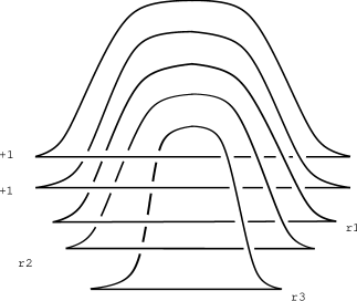
Figure 7: Contact structures on $Y(-1;r_{1},r_{2},r_{3})$

To understand the statement of Theorem 3.1 it is important to keep in mind that, since the rational numbers $-\frac{1}{r_{i}}$ are not necessarily of the form $\frac{1}{k}$, $k\in\mathbb{Z}$, the contact surgeries they determine are not unique (see Section 2). Therefore, for fixed $r_{1}$, $r_{2}$ and $r_{3}$, Figure 7 defines a finite collection of contact structures on the same underlying topological 3–manifold $Y(-1;r_{1},r_{2},r_{3})$. See [25, 26] for more details and explicit examples.

In [32] Ozsváth and Szabó prove the existence of an algorithm which computes ${{\widehat{HF}}}(Y)$ assuming that $Y$ is the boundary of a negative definite plumbing of a certain type. In Sections 4 and 5 we will use the Ozsváth–Szabó algorithm to apply Theorem 3.1. In order to state our next result we need to recall the main ingredient of the algorithm, that is the definition of full path.

Suppose that $\mathcal{T}$ is a plumbing tree of spheres, $W_{\mathcal{T}}$ is the corresponding 4–manifold and $Y_{\mathcal{T}}=\partial W_{\mathcal{T}}$. A vertex $v$ of $\mathcal{T}$ is bad if its valency is larger than the absolute value of its weight. The algorithm exists assuming that $\mathcal{T}$ is negative definite and has at most one bad vertex. Observe that such assumptions are satisfied if $\mathcal{T}$ is equal to a weighted tree $\Gamma^{\prime}$ as in Figure 6. Fix an identification of the set of vertices of $\mathcal{T}$ with a set of standard generators of $H_{2}(W_{\mathcal{T}};\mathbb{Z})$, so that $\mathcal{T}$ coincides with the corresponding intersection graph. An $m$–tuple $(K_{1},\ldots,K_{m})$ of second cohomology elements on $W_{\mathcal{T}}$ is said to be a full path if

• each $K_{i}\in H^{2}(W_{\mathcal{T}};{\mathbb{Z}})$ is a characteristic element, that is,

  $$\langle K_{i},v\rangle\equiv v\cdot v\quad\bmod 2\quad\text{for every $v\in\mathcal{T}$};$$

• $K_{1}$ is an initial vector, that is, it satisfies

  $$v\cdot v+2\leq\langle K_{1},v\rangle\leq-v\cdot v\quad\text{for every $v\in\mathcal{T}$};$$

• For $i=1,\ldots,m-1$ the vector $K_{i+1}$ is given by

  $$K_{i+1}=K_{i}+2PD(v)$$

  for some $v\in\mathcal{T}$ satisfying $\langle K_{i},v\rangle=-v\cdot v$;

• $K_{m}$ is a terminal vector, that is

  $$v\cdot v\leq\langle K_{m},v\rangle\leq-v\cdot v-2\quad\text{for every $v\in\mathcal{T}$}.$$

Notice that the length $m$ of a full path might vary. For example, if $v\cdot v<-1$ for every $v$ then there is a vector $K$ which is both initial and terminal:

$$\langle K,v\rangle:=\begin{cases}0\quad\text{if $v\cdot v$ is even},\\ 1\quad\text{if $v\cdot v$ is odd}.\end{cases}$$

Therefore in this case there is always a full path with $m=1$. According to [32], a full path $(K_{1},\ldots,K_{m})$ determines a non–trivial element of ${{\widehat{HF}}}(Y_{\mathcal{T}})$ whose absolute degree can be computed using the formula

$$\frac{1}{4}(K_{i}^{2}+|\mathcal{T}|),$$ (3.1)

where $K_{i}$ is any element of the full path. Notice that the transformation rule defining $K_{i+1}$ from $K_{i}$ implies that $K_{i}^{2}=K_{i+1}^{2}$, therefore the choice of the vector in the full path is irrelevant when computing the degree.

The construction given in the following lemma will be crucial in Sections 4 and 5.

Lemma 3.2.

Let $Y=Y(-1;r_{1},r_{2},r_{3})=\partial W_{\Gamma}$ with $\Gamma$ as in Figure 3. Then, there exist a smooth, closed and oriented 4–manifold $R$ containing $Y$ as a smooth hypersurface and an open tubular neighborhood $\nu(Y)\subset R$ such that

$$R\setminus\nu(Y)=W_{\Gamma}\cup W_{\Gamma^{\prime}}.$$

Moreover, $R$ is orientation preserving diffeomorphic to a blown–up complex projective plane.

Proof.

Start by blowing up the complex projective plane ${\mathbb{C}}{\mathbb{P}}^{2}$ at the common intersection point $p$ of three distinct lines $\ell_{1}$, $\ell_{2}$ and $\ell_{3}$. The union of the exceptional class, the proper transforms $\tilde{\ell}_{i}$ of the $\ell_{i}$, $i=1,2,3$, and the proper transform $\tilde{\ell}$ of a line $\ell\subset{\mathbb{C}}{\mathbb{P}}^{2}$ with $p\not\in\ell$ provides a configuration of five rational curves inside the rational surface ${\mathbb{C}}{\mathbb{P}}^{2}\#\overline{\mathbb{C}}{\mathbb{P}}^{2}$. We can now blow up more times, starting at the three intersection points $\tilde{\ell}\cap\tilde{\ell}_{i}$, $i=1,2,3$, until we obtain a configuration of rational curves in the blown–up projective plane with intersection graph identical to $\Gamma$. This gives an embedding of the plumbing $W_{\Gamma}$ into a blown-up ${\mathbb{C}}{\mathbb{P}}^{2}$, which we take as our $R$. Then it is easy to check that $Y=\partial W_{\Gamma}$ embeds as a hypersurface in $R$ and it has an open tubular neighborhood $\nu(Y)$ such that $R\setminus\nu(Y)=W_{\Gamma}\cup W_{\Gamma^{\prime}}$. ∎

Recall that, given a contact structure $\xi$ on a Seifert fibered 3–manifold $Y$, $\xi$ is called a transverse contact structure if it can be isotoped until it is transverse everywhere to the fibers of the Seifert fibration on $Y$. Since transverse contact structures are symplectically fillable [22] and therefore tight, the existence question for Seifert fibered 3–manifolds is only open in the absence of transverse contact structures. The following statement gives a practical criterion for the existence of tight contact structures on Seifert fibered 3–manifolds which do not carry transverse contact structures. It will be applied in Sections 4 and 5.

Theorem 3.3.

Let $Y=Y(-1;r_{1},r_{2},r_{3})=\partial W_{\Gamma}$ with $\Gamma$ as in Figure 3 and $e(Y)>0$. Suppose that $Y$ does not carry transverse contact structures, and let $\xi$ be a contact structure on $Y$ given by a surgery diagram as in Figure 7. Let $R$ be a smooth, closed 4–manifold containing $Y$ as in Lemma 3.2, and let $c\in H^{2}(R;{\mathbb{Z}})$ be a characteristic cohomology class such that:

• $d_{3}(\xi)=\frac{1}{4}((c|_{W_{\Gamma}})^{2}-3\sigma(W_{\Gamma})-2b_{2}(W_{\Gamma}))+1$;

• $c|_{W_{\Gamma^{\prime}}}$ belongs to a full path on $W_{\Gamma^{\prime}}$;

• $c^{2}=\sigma(R)$.

Then, $c(Y,\xi)\neq 0$ and hence $\xi$ is tight.

Proof.

By Theorem 3.1 it suffices to check the equality $d_{3}(\xi)=d(Y,\mathbf{t}_{\xi})$. Since $e(Y)>0$, $Y$ is a rational homology sphere. Therefore we have the splitting

$$H^{2}(R;{\mathbb{Q}})\cong H^{2}(W_{\Gamma};{\mathbb{Q}})\oplus H^{2}(W_{\Gamma^{\prime}};{\mathbb{Q}})\ni c_{\Gamma}+c_{\Gamma^{\prime}}=c,$$

where $c_{\Gamma}$ and $c_{\Gamma^{\prime}}$ abbreviates $c|_{W_{\Gamma}}$ and $c|_{W_{\Gamma^{\prime}}}$, respectively. By a simple computation using the fact that $b_{2}^{+}(W_{\Gamma})=1$ and the first assumption on $c$ we have

$$d_{3}(\xi)=\frac{1}{4}(c_{\Gamma}^{2}-3\sigma(W_{\Gamma})-2b_{2}(W_{\Gamma}))+1=\frac{1}{4}(c^{2}_{\Gamma}-\sigma(W_{\Gamma})).$$ (3.2)

By the second assumption on $c$, the restriction $c_{\Gamma^{\prime}}$ determines a non–trivial element of ${{\widehat{HF}}}(-Y,\mathbf{t}_{\xi})$ which, by (3.1), has degree

$$\frac{1}{4}(c_{\Gamma^{\prime}}^{2}+|\Gamma^{\prime}|)=\frac{1}{4}(c_{\Gamma^{\prime}}^{2}+b_{2}(W_{\Gamma^{\prime}})).$$

Now observe that by assumption $Y$ has no transverse contact structures while, since $e(-Y)=-e(Y)<0$, $-Y$ does carry contact structures transverse to the Seifert fibration [22, Proposition 3.1]. Applying [26, Theorem 1.1] gives that $Y$ is an $L$–space, therefore

$$d(-Y,\mathbf{t}_{\xi})=\frac{1}{4}(c_{\Gamma^{\prime}}^{2}+b_{2}(W_{\Gamma^{\prime}}))=\frac{1}{4}(c^{2}_{\Gamma^{\prime}}-\sigma(W_{\Gamma^{\prime}})).$$ (3.3)

Adding Equations (3.2) and (3.3) and using the third assumption we get

$$d_{3}(\xi)+d(-Y,\mathbf{t}_{\xi})=\frac{1}{4}(c^{2}-\sigma(R))=0.$$ (3.4)

Since $d(Y,\mathbf{t}_{\xi})=-d(-Y,\mathbf{t}_{\xi})$, Identity (3.4) implies $d_{3}(\xi)=d(Y,\mathbf{t}_{\xi})$, and the tightness of $\xi$ follows applying Theorem 3.1. ∎

4 First application of the criterion

In this section we apply Theorem 3.3 to prove the following statement:

Theorem 4.1.

Let $Y=Y(-1;r_{1},r_{2},r_{3})$ with $e(Y)>0$, and suppose that $Y$ carries no transverse contact structures. Suppose that $1>r_{1}\geq r_{2}\geq r_{3}>0$ satisfy Expansions (2.1), and each of the following holds:

• $a_{1}=\cdots=a_{k}=2$ and either

  • $n_{1}=k$ or

  • $n_{1}>k$ and $a_{k+1}>2$;

• $c_{1}\geq b_{1}=k+2$;

• $n_{1}>1$;

• $n_{3}=1$.

Then, $Y$ carries a contact structure $\xi$ given by a surgery diagram as in Figure 7 and such that $c(Y,\xi)\neq 0$. In particular, $Y$ carries a tight contact structure.

Figure 8: The tree $\Gamma$ under the assumptions of Theorem 4.1

Let $Y=\partial W_{\Gamma}$ be a 3–manifold as in the statement of Theorem 4.1. The corresponding tree $\Gamma$ is illustrated in Figure 8, with $(-2)$–weights omitted. Therefore we have $-Y=\partial W_{\Gamma^{\prime}}$, where the dual plumbing tree $\Gamma^{\prime}$ given in Figure 9, with $(-2)$–weights omitted. Explicitely, we have:

• The central vertex of $\Gamma^{\prime}$ has weigth $-2$.

• The leg $L_{1}^{\prime}$ starts out with a vertex $w$ of weight $-e$. Moreover,

  $$e=\begin{cases}k+1\ \text{if}\ l(L^{\prime}_{1})=1,\\ k+2\ \text{if}\ l(L^{\prime}_{1})>1.\end{cases}$$

• The leg $L_{2}^{\prime}$ starts out with $k\geq 1$ vertices of weight $-2$, then has a vertex $v$ of weight $-b\leq-2$ and then possibly more vertices.

• The leg $L_{3}^{\prime}$ has length $l(L_{3}^{\prime})=c_{1}-1\geq k+1$, and each one of its vertices has weight $-2$.

Figure 9:  The dual tree $\Gamma^{\prime}$ in the case of Theorem 4.1

Observe that we always have $e\geq 3$. This is clear if $l(L^{\prime}_{1})>1$, because $k\geq 1$. On the other hand, if $l(L^{\prime}_{1})=1$ then $n_{1}=k$, and since we are assuming $n_{1}>1$ we have $e=k+1\geq 3$. Moreover, if $n_{2}=1$ then $b=2$ and $l(L^{\prime}_{2})=k+1$, while if $n_{2}>1$ then $b\geq 3$ and $l(L^{\prime}_{2})\geq k+1$.

From now on, we fix an identification of the set of vertices of $\Gamma$ and $\Gamma^{\prime}$ with, respectively, sets of generators for the second integral homology of $W_{\Gamma}$ and $W_{\Gamma^{\prime}}$, so that $\Gamma$ and $\Gamma^{\prime}$ are the corresponding intersection graphs. Let $R$ be the smooth 4–manifold of Lemma 3.2. We will now define a characteristic cohomology class $c\in H^{2}(R;\mathbb{Z})$ and a contact structure $\xi$ on $Y$ via a contact surgery diagram as in Figure 7, and then we will apply Theorem 3.3. Denote by $h$ and $e_{i}$ standard generators of $H_{2}(R;{\mathbb{Z}})$, where $h$ has square $+1$ and each $e_{i}$ has square $-1$. It is easy to see that under the map induced by the embedding $W_{\Gamma}\cup W_{\Gamma^{\prime}}\subset R$, up to renaming the $e_{i}$’s we have:

• The central vertex of $\Gamma$ goes to $e_{1}$,

• The central vertex of $\Gamma^{\prime}$ goes to $h-e_{2}-e_{3}-e_{4}$,

• The first vertex of each leg $L_{i}$, $i=1,2,3$, goes to a class of the form $h-e_{1}-e_{i+1}-\sum_{j}e_{j}$.

• All the other vertices of $\Gamma$ and $\Gamma^{\prime}$ go to classes of the form $e_{j}-\sum_{k}e_{k}$.

Denote by $z$ and $z^{\prime}$, respectively, the central vertices of $\Gamma$ and $\Gamma^{\prime}$. Let $x_{i}$, for $i=1,2,3$, be the first vertex of $L_{i}$, that is the vertex closest to $z$, and by $y^{\prime}_{i}$, for $i=1,2,3$, the last vertex of $L^{\prime}_{i}$, that is the vertex of $L^{\prime}_{i}$ most distant from $z^{\prime}$. Let $E=\{e_{i}\}\subset H_{2}(R;\mathbb{Z})$ be the set of exceptional classes. Let

$$L^{\prime}_{2}[k]:=\{\text{first $k$ vertices of $L^{\prime}_{2}$}\},$$

$$S:=\{e_{i}\in E\ |\ e_{i}\cdot u=0\ \text{for each}\ u\in L^{\prime}_{2}[k]\ \text{and}\ e_{i}\cdot u\neq 0\ \text{for some}\ u\in L^{\prime}_{2}\setminus L^{\prime}_{2}[k]\},$$

$$T:=\{e_{i}\in E\ |\ e_{i}\cdot u\neq 0\ \text{for some}\ u\in L_{3}^{\prime}\setminus\{y^{\prime}_{3}\}\},$$

and define the class $c\in H^{2}(R;{\mathbb{Z}})$ through its Poincaré dual by

$$\operatorname{PD}(c):=h-\sum_{e\in E}e+2\sum_{e\in S}e+2\sum_{e\in T}e.$$ (4.1)

Observe that by construction $S\cap T=\emptyset$, which gives $\langle c,e_{i}\rangle=\pm 1$ for every $e_{i}$. This immediately implies that $c$ is characteristic and $c^{2}=\sigma(R)$. A tedious but straightforward verification shows that $c$ evaluates on the vertices of $\Gamma$ and $\Gamma^{\prime}$ as follows:

• $\langle c,z\rangle=+1$,

• $\langle c,x_{1}\rangle=x_{1}\cdot x_{1}=-2$,

• if $u\in L_{1}\setminus\{x_{1}\}$ then $\langle c,u\rangle=u\cdot u+2$,

• $\langle c,x_{2}\rangle=x_{2}\cdot x_{2}+2=-k$,

• if $u\in L_{2}\setminus\{x_{2}\}$ then $\langle c,u\rangle=-u\cdot u-2$,

• $\langle c,x_{3}\rangle=-x_{3}\cdot x_{3}-2=c_{1}-2$,

• $\langle c,z^{\prime}\rangle=0$,

• if $u\in L_{1}^{\prime}$ then $\langle c,u\rangle=u\cdot u+2$,

• $\langle c,v\rangle=-v\cdot v=b$,

• if $u\in L^{\prime}_{2}[k]$ then $\langle c,u\rangle=u\cdot u+2=0$,

• if $u\in L^{\prime}_{2}\setminus(L^{\prime}_{2}[k]\cup\{v\})$ then $\langle c,u\rangle=-u\cdot u-2$,

• $\langle c,y^{\prime}_{3}\rangle=y^{\prime}_{3}\cdot y^{\prime}_{3}=-2$,

• if $u\in L^{\prime}_{3}\setminus\{y^{\prime}_{3}\}$ then $\langle c,u\rangle=u\cdot u+2=0$.

Define $\xi$ to be the contact structure given by the contact surgery diagram of Figure 10. By [4, 5], this diagram is equivalent to a contact surgery diagram as in Figure 7. Moreover, after converting each contact framing into a smooth framing, with a little Kirby calculus as e.g. in [25] it is easy to check that the underlying topological 3–manifold is $Y=\partial W_{\Gamma}$.

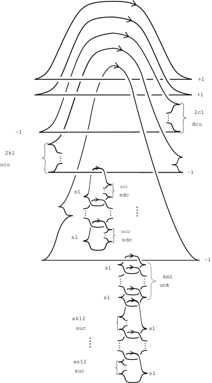
Figure 10: The contact structure $\xi$ used in the proof of Theorem 4.1.

Lemma 4.2.

We have

$$d_{3}(\xi)=\frac{1}{4}\left((c|_{W_{\Gamma}})^{2}-3\sigma(W_{\Gamma})-2b_{2}(W_{\Gamma})\right)+1.$$

Proof.

One can think of Figure 10 smoothly, as a handlebody presentation of a smooth 4–manifold $X$ having one 0–handle and a number of 2–handles. The knot orientations indicated in Figure 10 determine rotation numbers which, according to [17, 18], can be computed by the formula

$${\rm{rot}}(K)=\frac{1}{2}(c_{d}-c_{u}),$$ (4.2)

where $c_{u}$ and $c_{d}$ denote the number of up and down cusps, respectively, in the front projection of $K$. Let $\alpha\in H^{2}(X;\mathbb{Z})$ be the unique cohomology class which evaluates on the 2–homology class corresponding to an oriented knot $K$ of the diagram as the rotation number of $K$. By [6, Corollary 3.6] (with the Euler characteristic $\chi$ replaced by the second Betti number $b_{2}$ to adjust for the standard convention in Heegaard Floer theory) we have

$$d_{3}(\xi)=\frac{1}{4}(\alpha^{2}-3\sigma(X)-2b_{2}(X))+2.$$

An easy exercise in Kirby calculus shows that there is a orientation–preserving diffeomorphism $\varphi\co X\#{\mathbb{C}}{\mathbb{P}}^{2}\cong{W_{\Gamma}}\#2{\mathbb{C}}{\mathbb{P}}^{2}$. Therefore we have

$$b_{2}(X)=b_{2}(W_{\Gamma})+1\quad\text{and}\quad\sigma(X)=\sigma(W_{\Gamma})+1.$$

Moreover, we can define the extension $\tilde{\alpha}\in H^{2}(X\#{\mathbb{C}}{\mathbb{P}}^{2};\mathbb{Z})$ of $\alpha$ by declaring its value on the standard generator of the 2–homology of the ${\mathbb{C}}{\mathbb{P}}^{2}$–summand to be $-1$. It is easy to check that for a natural choice of $\varphi$ the class $\varphi_{*}(\tilde{\alpha})$ takes value $-1$ on the standard generator of each ${\mathbb{C}}{\mathbb{P}}^{2}$–summand, and $\varphi_{*}(\tilde{\alpha})|_{W_{\Gamma}}=c|_{W_{\Gamma}}$. Therefore

$$(c|_{W_{\Gamma}})^{2}+2=\varphi_{*}(\tilde{\alpha})^{2}=(\tilde{\alpha})^{2}=\alpha^{2}+1,$$

which implies $\alpha^{2}=(c|_{W_{\Gamma}})^{2}+1$. Thus, we conclude

$$d_{3}(\xi)=\frac{1}{4}((c|_{W_{\Gamma}})^{2}+1-3(\sigma(W_{\Gamma})+1)-2(b_{2}(W_{\Gamma})+1))+2=\\ =\frac{1}{4}\left((c|_{W_{\Gamma}})^{2}-3\sigma(W_{\Gamma})-2b_{2}(W_{\Gamma})\right)+1.$$

∎

In order to apply Theorem 3.3 and conclude that the contact structure $\xi$ has non–zero contact invariant, thus proving Theorem 4.1, it now suffices to check that, when restricted to $W_{\Gamma^{\prime}}$, the class $c$ is contained in a full path on $\Gamma^{\prime}$. The nonzero values of $c$ on $\Gamma^{\prime}$ are shown in parenthesis in Figure 11.

Figure 11:  The nonzero values of $c$

In what follows it will be convenient to introduce shorthands to keep track of the values of cohomology classes such as $c$. For example, we can express the information contained in Figure 11 as follows:

$$\begin{matrix}&&0&\cdots&0&(-2)&\\ (2-d)\ \cdots\ (2-e)&0&&&&&\\ &&0&\cdots&0&b&\cdots\ (d^{\prime}-2)\end{matrix}$$

Lemma 4.3.

The vector of values defined by $c$ on $\Gamma^{\prime}$ is contained in a full path.

Proof.

Throughout the proof we will identify, when convenient, characteristic classes with their sets of values on the standard homology generators. Observe that the value $-2$ on $y^{\prime}_{3}$ prevents $c$ from being initial, and the value $b$ on $v$ prevents $c$ from being terminal.

We start by showing that there is a sequence of characteristic classes from $c$ to a terminal vector $L$. Recall from Section 3 that this means

$$u\cdot u\leq L\cdot u\leq-u\cdot u-2$$

for every vertex $u$. Replacing $c$ with $c+2\operatorname{PD}(v)$ creates value $-b$ on $v$, $+2$ on the vertex of position $k$ on $L_{2}^{\prime}$ and, if $l(L_{2}^{\prime})>k+1$, value $f$ on the vertex to the right of $v$, of position $k+2$ on $L_{2}^{\prime}$ (assuming its weight is $-f$). The resulting set of values can be represented as follows:

$$\begin{matrix}&&0&\cdots&0&(-2)&\\ (2-d)\ \cdots\ (2-e)&0&&&&&\\ &&0&\cdots&2&(-b)&f\cdots\ (d^{\prime}-2)\end{matrix}$$

By a sequence of similar operations we obtain

$$\begin{matrix}&&0&\cdots\ 0&(-2)&&\\ (2-d)\ \cdots\ (2-e)&0&&&&&\\ &&0&\cdots\ 2&(-2)&(2-b)&f\cdots\ (d^{\prime}-2)\end{matrix}$$

$$\vdots$$

$$\begin{matrix}&&0&\cdots&0&(-2)&\\ (2-d)\ \cdots\ (2-e)&2&&&&&\\ &&(-2)&\cdots&0&(2-b)&f\cdots\ (d^{\prime}-2)\end{matrix}$$

Adding twice the Poincaré dual of the homology class corresponding to the central vertex we get

$$\begin{matrix}&&2&\cdots&0&(-2)&\\ (2-d)\ \cdots\ (4-e)&(-2)&&&&&\\ &&0&\cdots&0&(2-b)&f\cdots\ (d^{\prime}-2)\end{matrix}$$

Notice that $4-e$ is an admissible value for a class in a full path, that is

$$-e<-e+4<e,$$

because we are assuming $e\geq 3$. By another sequence of similar operations we arrive at

$$\begin{matrix}&&0&\cdots\ (-2)&2&(-2)&\\ (2-d)\ \cdots\ (4-e)&0&&&&&\\ &&0&\cdots&0&(2-b)&f\cdots\ (d^{\prime}-2)\end{matrix}$$

and then at

$$\begin{matrix}&&0&\cdots\ 0&(-2)&0&\\ (2-d)\ \cdots\ (4-e)&0&&&&&\\ &&0&\cdots&0&(2-b)&f\cdots\ (d^{\prime}-2)\end{matrix}$$

If $l(L_{2}^{\prime})>k+1$ we need to deal with the value $f$ on the vertex at position $k+2$ on $L_{2}^{\prime}$. Recall that $l(L^{\prime}_{2})>k+1$ occurs only if $b\geq 3$. Therefore we can proceed to

$$\begin{matrix}&&0&\cdots\ 0&(-2)&0&\\ (2-d)\ \cdots\ (4-e)&0&&&&&\\ &&0&\cdots&0&(4-b)&(-f)\ g\cdots\ (d^{\prime}-2)\end{matrix}$$

where we are assuming that the value of the vertex of position $k+3$ exists and has weight $-g$ (if such vertex does not exist, we are done). Notice that the value $4-b$ is good because $b\geq 3$. If we keep going like this we eventually arrive at the vector $L$ given by

$$\begin{matrix}&&0&\cdots\ 0&(-2)&0&\\ (2-d)\ \cdots\ (4-e)&0&&&&&\\ &&0&\cdots&0&(4-b)&(2-f)\ (2-g)\cdots\ (-d^{\prime})\end{matrix}$$

The vector $L$ is terminal in the sense of Section 3. The above argument shows that, regardless of whether $l(L^{\prime}_{2})=k+1$ or $l(L^{\prime}_{2})>k+1$, we can always find a path joining $c$ to such a terminal vector. This concludes the first half of the proof.

In the second part of the proof we show the existence of a path joining $c$ back to an initial vector $K$ in the sense of Section 3. At each step now we are subtracting, instead of adding, twice the Poincaré dual of a homology class corresponding to a vertex. Since there is no new conceptual ingredient involved, we present just the shorthand description of the various steps, commenting only when strictly necessary.

$$c=\begin{matrix}&&0&\cdots&0&(-2)&\\ (2-d)\ \cdots\ (2-e)&0&&&&&\\ &&0&\cdots&0&b&\cdots\ (d^{\prime}-2)\end{matrix}$$

$$\longrightarrow\ \begin{matrix}&&0&\cdots&(-2)&2&\\ (2-d)\ \cdots\ (2-e)&0&&&&&\\ &&0&\cdots&0&b&\cdots\ (d^{\prime}-2)\end{matrix}$$

$$\longrightarrow\ \cdots\longrightarrow\ \begin{matrix}&&2&\cdots&0&0&\\ (2-d)\ \cdots\ (2-e)&(-2)&&&&&\\ &&0&\cdots&0&b&\cdots\ (d^{\prime}-2)\end{matrix}$$

$$\longrightarrow\ \begin{matrix}&&0&\cdots&0&0&\\ (2-d)\ \cdots\ (-e)&2&&&&&\\ &&(-2)&\cdots&0&b&\cdots\ (d^{\prime}-2)\end{matrix}$$

$$\longrightarrow\ \cdots\longrightarrow\ \begin{matrix}&&0&\cdots&0&0&\\ (2-d)\ \cdots\ (-e)&0&&&&&\\ &&0&\cdots\ 2&(-2)&b&\cdots\ (d^{\prime}-2)\end{matrix}$$

$$\longrightarrow\ \begin{matrix}&&0&\cdots&0&0&\\ (2-d)\ \cdots\ (-e)&0&&&&&\\ &&0&\cdots&2&(b-2)&\cdots\ (d^{\prime}-2)\end{matrix}$$

$$\longrightarrow\ \begin{matrix}&&0&\cdots&0&0&\\ (2-d)\ \cdots\ (-h)\ e&(-2)&&&&&\\ &&0&\cdots&2&(b-2)&\cdots\ (d^{\prime}-2)\end{matrix}$$

where we are assuming that the second vertex of $L_{1}^{\prime}$ exists and has weight $-h$. Still assuming that $l(L^{\prime}_{1})>1$, we eventually arrive at the configuration:

$$U=\begin{matrix}&&0&\cdots&0&0&\\ d\ \cdots\ (h-2)\ (e-2)&(-2)&&&&&\\ &&0&\cdots&2&(b-2)&\cdots\ (d^{\prime}-2)\end{matrix}$$

On the other hand, if $l(L^{\prime}_{1})=1$ at this point we have the set of values:

$$V=\begin{matrix}&&0&\cdots&0&0&\\ e&(-2)&&&&&\\ &&0&\cdots&2&(b-2)&\cdots\ (d^{\prime}-2)\end{matrix}$$

In case $(A)$ there are two subcases: $k=1$ and $k>1$. If $k=1$ we proceed as follows:

$$U\ =\ \begin{matrix}&&0&\cdots\ 0&\\ d\ \cdots\ (h-2)\ (e-2)&(-2)&&&\\ &&2&(b-2)&\cdots\ (d^{\prime}-2)\end{matrix}$$

$$\longrightarrow\ \begin{matrix}&&(-2)&\cdots\ 0&\\ d\ \cdots\ (h-2)\ (e-4)&2&&&\\ &&0&(b-2)&\cdots\ (d^{\prime}-2)\end{matrix}$$

$$\longrightarrow\ \cdots\longrightarrow\ \begin{matrix}&&0&\cdots\ 2&\\ d\ \cdots\ (h-2)\ (e-4)&0&&&\\ &&0&(b-2)&\cdots\ (d^{\prime}-2)\end{matrix}\ =\ K.$$

Observe that this vector $K$ is initial, therefore in this subcase we are done. Notice that in case $(B)$ $e\geq 3$ forces $k>1$, therefore from now on we assume $k>1$ in both cases $(A)$ and $(B)$. In case $(A)$ we proceed as follows:

$$U=\begin{matrix}&&0&\cdots&0&0&\\ d\ \cdots\ (h-2)\ (e-2)&(-2)&&&&&\\ &&0&\cdots&2&(b-2)&\cdots\ (d^{\prime}-2)\end{matrix}$$

$$\longrightarrow\ \begin{matrix}&&(-2)&\cdots&0&0&\\ d\ \cdots\ (h-2)\ (e-4)&2&&&&&\\ &&(-2)&\cdots&2&(b-2)&\cdots\ (d^{\prime}-2)\end{matrix}$$

$$\longrightarrow\ \cdots\longrightarrow\ \begin{matrix}&&(-2)&\cdots&0&0&\\ d\ \cdots\ (h-2)\ (e-4)&0&&&&&\\ &&0&\cdots\ 2&0&(b-2)&\cdots\ (d^{\prime}-2)\end{matrix}$$

$$\longrightarrow\ \begin{matrix}&&2&(-2)\ \cdots&0&0&\\ d\ \cdots\ (h-2)\ (e-4)&(-2)&&&&&\\ &&0&\cdots\ 2&0&(b-2)&\cdots\ (d^{\prime}-2)\end{matrix}$$

$$\longrightarrow\ \begin{matrix}&&0&(-2)\ \cdots&0&0&\\ d\ \cdots\ (h-2)\ (e-6)&2&&&&&\\ &&(-2)&\cdots\ 2&0&(b-2)&\cdots\ (d^{\prime}-2)\end{matrix}$$

$$\longrightarrow\ \cdots\longrightarrow\ \begin{matrix}&&0&(-2)\ \cdots\ 0\ 0&\\ d\ \cdots\ (h-2)\ (e-6)&0&&&&&\\ &&0&\cdots\ 2\ 0\ 0\ (b-2)&\cdots\ (d^{\prime}-2)\end{matrix}$$

$$\longrightarrow\ \cdots\longrightarrow\ \begin{matrix}&&\overbrace{0\ \cdots\ (-2)\ 2\ (-2)}^{t+1}\ \cdots\ 0\phantom{xxxxx}&\\ d\ \cdots\ (h-2)\ (e-2t-2)&0&&\\ &&\underbrace{0\ \cdots\ 2}_{k-t}\ \cdots\ (b-2)\ \cdots\ (d^{\prime}-2)&\end{matrix}$$

In case $(B)$ similar steps lead to

$$\begin{matrix}&&\overbrace{0\ \cdots\ (-2)\ 2\ (-2)}^{t+1}\ \cdots\ 0\phantom{xxxxx}&\\ (e-2t)&0&&\\ &&\underbrace{0\ \cdots\ 2}_{k-t}\ \cdots\ (b-2)\ \cdots\ (d^{\prime}-2)&\end{matrix}$$

Since by assumption $e=k+2$ in case $(A)$ and $e=k+1$ in case $(B)$, choosing $t=k-1$ at this point leads, in both cases $(A)$ and $(B)$, to the vector

$$\begin{matrix}&&\overbrace{0\ \cdots\ (-2)\ 2\ (-2)}^{k}\ \cdots\ 0\phantom{xxx}&\\ d\ \cdots\ (h-2)\ (4-e)&0&&\\ &&2\ 0\ \cdots\ 0\ (b-2)\ \cdots\ (d^{\prime}-2)&\end{matrix}$$

Then, we proceed as follow

$$\longrightarrow\ \cdots\longrightarrow\ \begin{matrix}&&\overbrace{2\ \cdots\ 0\ (-2)}^{k}\ \cdots\ 0\phantom{xxxxxxx}&\\ d\ \cdots\ (h-2)\ (4-e)&(-2)&&\\ &&2\ 0\ \cdots\ 0\ (b-2)\ \cdots\ (d^{\prime}-2)&\end{matrix}$$

$$\longrightarrow\ \cdots\longrightarrow\ \begin{matrix}&&\overbrace{0\ \cdots\ 0\ (-2)}^{k}\ \cdots\ 0\phantom{xxxxxx}&\\ d\ \cdots\ (h-2)\ (2-e)&2&&\\ &&0\ \cdots\ 0\ (b-2)\ \cdots\ (d^{\prime}-2)&\end{matrix}$$

$$\longrightarrow\ \begin{matrix}&&\overbrace{0\ \cdots\ (-2)\ (2)}^{k}\ (-2)\cdots\ 0\phantom{xx}&\\ d\ \cdots\ (h-2)\ (2-e)&2&&\\ &&0\ \cdots\ 0\ (b-2)\ \cdots\ (d^{\prime}-2)&\end{matrix}$$

$$\longrightarrow\ \cdots\longrightarrow\ \begin{matrix}&&2\ \overbrace{0\ \cdots\ 0\ (-2)}^{k}\ 0\cdots\ 0\phantom{xxx}&\\ d\ \cdots\ (h-2)\ (2-e)&0&&\\ &&0\ \cdots\ 0\ (b-2)\ \cdots\ (d^{\prime}-2)&\end{matrix}$$

$$\longrightarrow\ \overset{(\text{$t-1$ steps})}{\cdots}\longrightarrow\ \begin{matrix}&&\overbrace{0\ \cdots\ 0\ 2}^{t}\ \overbrace{0\ \cdots\ 0\ (-2)}^{k}\ 0\cdots\ 0&\\ d\ \cdots\ (h-2)\ (2-e)&0&&\\ &&0\ \cdots\ 0\ (b-2)\ \cdots\ (d^{\prime}-2)\phantom{xxx}&\end{matrix}$$

$$\longrightarrow\ \cdots\longrightarrow\ \begin{matrix}&&\overbrace{0\ \cdots\ 0\ 2}^{l(L^{\prime}_{3})-k}\ \overbrace{0\ \cdots\ 0\ (-2)}^{k}\phantom{xxx}&\\ d\ \cdots\ (h-2)\ (2-e)&0&&\\ &&0\ \cdots\ 0\ (b-2)\ \cdots\ (d^{\prime}-2)&\end{matrix}$$

$$\longrightarrow\ \begin{matrix}&&\overbrace{0\ \cdots\ 0\ 2}^{l(L^{\prime}_{3})-k}\ \overbrace{0\ \cdots\ (-2)\ 2}^{k}\phantom{xx}&\\ d\ \cdots\ (h-2)\ (2-e)&0&&\\ &&0\ \cdots\ 0\ (b-2)\ \cdots\ (d^{\prime}-2)&\end{matrix}$$

$$\longrightarrow\ \cdots\longrightarrow\ \begin{matrix}&&0&\cdots&0&\overbrace{2\ \cdots\ 0}^{k}&&\\ d\ \cdots\ (h-2)\ (2-e)&0&&&&&&\\ &&0&\cdots&0&(b-2)\ \cdots&(d^{\prime}-2)&\end{matrix}\ =\ K$$

Clearly $K$ is an initial vector, so this concludes the proof of the existence of the full path. ∎

Proof of Theorem 4.1.

By the assumptions on $Y$ and Lemmas 4.2 and 4.3, Theorem 3.3 applies. Therefore we conclude that the contact structure $\xi$ defined in Figure 10 has nonzero contact invariant. ∎

5 Second application of the criterion

In this section we apply Theorem 3.3 to prove Theorem 5.1 below.

Theorem 5.1.

Let $Y=Y(-1;r_{1},r_{2},r_{3})$ with $e(Y)>0$, and suppose that $Y$ carries no transverse contact structures. Suppose that $1>r_{1}\geq r_{2}\geq r_{3}>0$ satisfy Expansions (2.1) and each of the following holds:

• $n_{1}=1$ and $a_{1}=2$;

• $c_{1}\geq b_{1}=3$;

• $n_{3}=1$.

Then, either $Y\cong M_{n}$ for some $n\geq 1$ or $Y$ carries a contact structure $\xi$ given by a surgery diagram as in Figure 7 and such that $c(Y,\xi)\neq 0$.

Under the assumptions of Theorem 5.1 we have $Y=W_{\Gamma}$, where the tree $\Gamma$ takes the form given in Figure 12.

Figure 12:  The tree $\Gamma$ under the assumptions of Theorem 5.1

Lemma 5.2.

To prove Theorem 5.1 it suffices to prove the statement under the following extra assumptions:

• $c_{1}=2s+5$;

• $n_{2}=s+2$,

where $s\geq 0$ is the number of $(-2)$–vertices on $L_{2}$ after the first vertex.

Proof.

Let $Y=Y(-1;r_{1},r_{2},r_{3})$ with $e(Y)>0$, suppose that $Y$ carries no transverse contact structures and the $r_{i}$ satisfy the assumptions of Theorem 5.1. We will argue as in Proposition 2.2, viewing the weighted tree as prescribing an integral surgery presentation for $Y=\partial W_{\Gamma}$. We successively blow down $(-1)$–framed unknots by starting with the central one, continuing with the unique vertex of $L_{1}$ and then with the first $s+1$ vertices on $L_{2}$. In this way we obtain a link consisting of a $(2,2s+3)$–torus knot, linked positively twice to an unknot if $n_{2}>s+1$, plus a further chain of unknots if $n_{2}>s+2$.

By [24] we know that if the smooth surgery coefficient $\gamma=-c_{1}+2+4(s+1)$ on the $(2,2s+3)$–torus knot $T_{2,2s+3}$ is not equal to $2s+1$, then the 3–manifold $N=S^{3}_{\gamma}(T_{2,2s+3})$ carries a contact structure $\zeta$ with $c(N,\zeta)\neq 0$ obtained by contact $(\gamma-2s-1)$–surgery on a Legendrian $(2,2s+3)$–torus knot with Thurston–Bennequin invariant $2s+1$ in the standard contact $S^{3}$. Since the smooth framings of the unknots are all $\leq-2$ and all linking numbers are non–negative, the corresponding topological surgeries can all be realized by contact $(-1)$–surgeries. Thus, arguing as in Proposition 2.2 we see that if $\gamma\neq 2s+1$ (equivalently, $c_{1}\neq 2s+5$) then $Y$ carries a contact structure $\xi$ such that $c(Y,\xi)\neq 0$. Since by assumption $Y$ carries no transverse contact structures, by [13, Theorem 1.2] the contact structure $\xi$ has maximal twisting $t(\xi)=0$. This implies, by [26, Proposition 6.1], that $\xi$ is given by a surgery diagram as in Figure 7. Therefore, the conclusion of Theorem 5.1 holds for $Y$ and we see that the extra assumption $c_{1}=2s+5$ leads to no loss of generality. Moreover, if $c_{1}=2s+5$ and $n_{2}=s+1$ then $Y\cong M_{n_{2}}$. Thus, we may assume without loss that $c_{1}=2s+5$ and $n_{2}>s+1$.

Finally, we observe that it suffices to assume $n_{2}=s+2$. In fact, suppose that each manifold $Z$ corresponding to $n_{2}=s+2$ carries a contact structure $\eta$ given by a surgery diagram as in Figure 7 with $c(Z,\eta)\neq 0$. Then, arguing as before it is easy to see that each manifold $Y$ corresponding to $n_{2}>s+2$ can be obtained as the underlying 3–manifold of a contact $(-1)$–surgery on some $(Z,\eta)$. This concludes the proof. ∎

By Lemma 5.2, in order to finish the proof of Theorem 5.1 it suffices to consider trees $\Gamma$ as in Figure 13 and dual trees $\Gamma^{\prime}$ as in Figure 14, where unmarked vertices have weight $-2$.

Figure 13: The tree $\Gamma$ under the assumptions of Theorem 5.1 and Lemma 5.2

Figure 14: The tree $\Gamma^{\prime}$ under the assumptions of Theorem 5.1 and Lemma 5.2

By Lemma 3.2 there exists a smooth, closed 4–manifold $R$ containing $Y$ as a hypersurface, with an open tubular neighborhood $\nu(Y)\subset R$ such that $R\setminus\nu(Y)=W_{\Gamma}\cup W_{\Gamma^{\prime}}$. Arguing as in the previous section, we now define a characteristic cohomology class $c\in H^{2}(R;\mathbb{Z})$ and a contact structure $\xi$ on $Y$ given by a contact surgery diagram as in Figure 7. Then, we will apply Theorem 3.3.

Fix an identification of the set of vertices of $\Gamma$ and $\Gamma^{\prime}$ with, respetively, sets of generators for the second integral homology of $W_{\Gamma}$ and $W_{\Gamma^{\prime}}$, so that $\Gamma$ and $\Gamma^{\prime}$ are the corresponding intersection graphs. Denote by $h$ and $e_{i}$ standard generators of $H_{2}(R;{\mathbb{Z}})$, where $h$ has square $+1$ and each $e_{i}$ has square $-1$. Under the map induced by the embedding $W_{\Gamma}^{\prime}\cup W_{\Gamma^{\prime}}\subset R$, up to renaming the $e_{i}$’s we have:

• The central vertex of $\Gamma$ goes to $e_{1}$,

• The central vertex of $\Gamma^{\prime}$ goes to $h-e_{2}-e_{3}-e_{4}$,

• The first vertex $x_{i}$ of each leg $L_{i}$, $i=1,2,3$, goes to a class of the form $h-e_{1}-e_{i+1}-\sum_{j}e_{j}$.

• All the other vertices go to classes of the form $e_{j}-\sum_{i}e_{i}$.

Denote by $x^{\prime}_{2}$ the first vertex of $L^{\prime}_{2}$, by $y^{\prime}_{3}$ the last vertex of $L^{\prime}_{3}$ and by $v$ the vertex indicated in Figure 14. Let $E=\{e_{i}\}$ be the set of exceptional classes. We define a class $c\in H^{2}(R;\mathbb{Z})$ by the formula

$$\operatorname{PD}(c):=h-\sum_{e\in E}e+2\sum_{e\in T}e+2\sum_{e\in S^{\prime}}e,$$

where $E$ is the set of exceptional classes,

$$T:=\{e_{i}\in E\ |\ e_{i}\cdot u\neq 0\ \text{for some}\ u\in L_{3}^{\prime}\setminus\{y^{\prime}_{3}\}\}$$

and

$$S^{\prime}:=\{e_{i}\in E\ |\ e_{i}\cdot u\neq 0\ \text{for every}\ u\in L^{\prime}_{2}\setminus\{v,x^{\prime}_{2}\}\ \text{and}\ e_{i}\cdot x^{\prime}_{2}=e_{i}\cdot v=0\}.$$

Observe that by construction $S\cap T=\emptyset$, which gives $\langle c,e_{i}\rangle=\pm 1$ for every $e_{i}$. This immediately implies that $c$ is characteristic and $c^{2}=\sigma(R)$. When restricted to $W_{\Gamma}$, the class $c$ takes the values given by

$$\begin{matrix}&(-2)&\\ (2s+3)&1&(-3)\ 0\ \cdots\ 0\ (m-2).\end{matrix}$$

Define $\xi$ to be the contact structure defined by the contact surgery diagram of Figure 15. By [4, 5], this diagram is equivalent to a contact surgery diagram as in Figure 7. Moreover, with a little Kirby calculus as in Section 4 it is easy to check that the underlying topological 3–manifold is $Y=\partial W_{\Gamma}$.

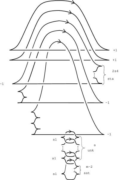
Figure 15: The contact structure $\xi$ used in the proof of Lemma 5.2

Lemma 5.3.

We have

$$d_{3}(\xi)=\frac{1}{4}\left((c|_{W_{\Gamma}})^{2}-3\sigma(W_{\Gamma})-2b_{2}(W_{\Gamma})\right)+1.$$

Proof.

The proof is exactly the same as the proof of Lemma 4.2, so here we only outline the argument. When viewed smoothly, Figure 15 gives a handlebody presentation of a smooth 4–manifold $X$ with one 0–handle and a number of 2–handles. The rotation numbers associated with every Legendrian knot determine a cohomology class $\alpha\in H^{2}(Z;\mathbb{Z})$ such that

$$d_{3}(\xi)=\frac{1}{4}(\alpha^{2}-3\sigma(X)-2b_{2}(X))+2=\\ =\frac{1}{4}\left((c|_{W_{\Gamma}})^{2}-3\sigma(W_{\Gamma})-2b_{2}(W_{\Gamma})\right)+1.$$ (5.1)

∎

Now we want to check that, when restricted to $W_{\Gamma^{\prime}}$, the class $c$ gives a vector of values $V$ contained in a full path on $\Gamma^{\prime}$. We have:

$$V\ =\ \begin{matrix}&0&\\ (-2)\ 0\ \cdots\ 0&0&0\ (-s-1)\ 2\ 0\cdots\ 0\end{matrix}$$

Lemma 5.4.

The vector $V$ of values defined by $c$ on $\Gamma^{\prime}$ is contained in a full path.

Proof.

Observe that the values preventing $V$ from being a terminal, respectively an intial vector are $2$ and, respectively $-2$. We start by constructing the lower part of the full path from $V$ to a terminal vector $L$:

$$V=\begin{matrix}&0&\\ (-2)\ 0\ \cdots\ 0&0&0\ (-s-1)\ 2\ 0\cdots\ 0\end{matrix}$$

$$\longrightarrow\ \begin{matrix}&0&\\ (-2)\ 0\ \cdots\ 0&0&0\ (-s+1)\ (-2)\ 2\ \cdots\ 0\end{matrix}$$

$$\longrightarrow\ \cdots\longrightarrow\ \begin{matrix}&0&\\ (-2)\ 0\ \cdots\ 0&0&0\ (-s+1)\ 0\ \cdots\ (-2)\ 2\end{matrix}$$

$$\longrightarrow\ \begin{matrix}&0&\\ (-2)\ 0\ \cdots\ 0&0&0\ (-s+1)\ 0\ \cdots\ 0\ (-2)\end{matrix}\ =\ L$$

Observe that $L$ is an terminal vector because, since $s\geq 0$, we have

$$-s-3<-s+1<s+3.$$

Now we construct the upper part of the full path, connecting $V$ to an initial vector $K$:

$$V=\begin{matrix}&0&\\ (-2)\ 0\ \cdots\ 0&0&0\ (-s-1)\ 2\ \cdots\ 0\end{matrix}$$

$$\longrightarrow\ \begin{matrix}&0&\\ 2\ (-2)\ \cdots\ 0&0&0\ (-s-1)\ 2\ \cdots\ 0\end{matrix}$$

$$\longrightarrow\ \cdots\longrightarrow\ \begin{matrix}&0&\\ 0\ 0\ \cdots\ 2&(-2)&0\ (-s-1)\ 2\ \cdots\ 0\end{matrix}$$

$$\longrightarrow\ \begin{matrix}&(-2)&\\ 0\ 0\ \cdots\ 0&2&(-2)\ (-s-1)\ 2\ \cdots\ 0\end{matrix}$$

$$\longrightarrow\ \begin{matrix}&(-2)&\\ 0\ 0\ \cdots\ 0&0&2\ (-s-3)\ 2\ \cdots\ 0\end{matrix}$$

$$\longrightarrow\ \begin{matrix}&(-2)&\\ 0\ 0\ \cdots\ 0&0&0\ (s+3)\ 0\ \cdots\ 0\end{matrix}$$

$$\longrightarrow\ \begin{matrix}&2&\\ 0\ 0\ \cdots\ 0&(-2)&0\ (s+3)\ 0\ \cdots\ 0\end{matrix}$$

$$\longrightarrow\ \begin{matrix}&0&\\ 0\ 0\ \cdots\ (-2)&2&(-2)\ (s+3)\ 0\ \cdots\ 0\end{matrix}$$

$$\longrightarrow\ \cdots\longrightarrow\ \begin{matrix}&0&\\ 2\ 0\ \cdots\ 0&0&(-2)\ (s+3)\ 0\ \cdots\ 0\end{matrix}$$

$$\longrightarrow\ \begin{matrix}&0&\\ 2\ 0\ \cdots\ 0&(-2)&2\ (s+1)\ 0\ \cdots\ 0\end{matrix}$$

$$\longrightarrow\ \begin{matrix}&(-2)&\\ 2\ 0\ \cdots\ (-2)&2&0\ (s+1)\ 0\ \cdots\ 0\end{matrix}$$

$$\longrightarrow\ \cdots\longrightarrow\ \begin{matrix}&(-2)&\\ 0\ 2\ \cdots\ 0&0&0\ (s+1)\ 0\ \cdots\ 0\end{matrix}$$

$$\longrightarrow\ \begin{matrix}&2&\\ 0\ 2\ \cdots\ 0&(-2)&0\ s+1\ 0\ \cdots\ 0\end{matrix}$$

$$\longrightarrow\ \begin{matrix}&0&\\ 0\ 2\ \cdots\ (-2)&2&(-2)\ s+1\ 0\ \cdots\ 0\end{matrix}$$

$$\longrightarrow\ \cdots\longrightarrow\ \begin{matrix}&0&\\ 0\ 0\ 2\cdots\ 0&0&(-2)\ (s+1)\ 0\ \cdots\ 0\end{matrix}$$

$$\longrightarrow\ \begin{matrix}&0&\\ 0\ 0\ 2\cdots\ 0&(-2)&2\ (s-1)\ 0\ \cdots\ 0\end{matrix}$$

$$\longrightarrow\ \begin{matrix}&(-2)&\\ 0\ 0\ 2\cdots\ (-2)&2&0\ (s-1)\ 0\ \cdots\ 0\end{matrix}$$

$$\longrightarrow\ \cdots\longrightarrow\ \begin{matrix}&(-2)&\\ \underbrace{0\ \cdots\ 2}_{2t+1}\cdots\ (-2)&2&0\ (s+1-2t)\ 0\ \cdots\ 0\end{matrix}$$

For $t=s+1$ we get

$$\begin{matrix}&(-2)&\\ 0\ \cdots\ 2\ (-2)&2&0\ (-s-1)\ 0\ \cdots\ 0\end{matrix}$$

$$\longrightarrow\ \begin{matrix}&(-2)&\\ 0\ \cdots\ 0\ 2&0&0\ (-s-1)\ 0\ \cdots\ 0\end{matrix}$$

$$\longrightarrow\ \begin{matrix}&2&\\ 0\ \cdots\ 0\ 2&(-2)&0\ (-s-1)\ 0\ \cdots\ 0\end{matrix}$$

$$\longrightarrow\ \begin{matrix}&0&\\ 0\ \cdots\ 0\ 0&2&(-2)\ (-s-1)\ 0\ \cdots\ 0\end{matrix}$$

$$\longrightarrow\ \begin{matrix}&0&\\ 0\ \cdots\ 0\ 0&0&2\ (-s-3)\ 0\ \cdots\ 0\end{matrix}$$

$$\longrightarrow\ \begin{matrix}&0&\\ 0\ \cdots\ 0\ 0&0&0\ (s+3)\ (-2)\ \cdots\ 0\end{matrix}$$

$$\longrightarrow\ \begin{matrix}&0&\\ 0\ \cdots\ 0\ 0&0&0\ (s+1)\ (2)\ (-2)\ \cdots\ 0\end{matrix}$$

$$\longrightarrow\ \cdots\longrightarrow\ \begin{matrix}&0&\\ 0\ \cdots\ 0\ 0&0&0\ (s+1)\ 0\ \cdots\ 0\ 2\end{matrix}=K.$$

∎

Proof of Theorem 5.1.

By the assumptions on $Y$ and Lemmas 5.3 and 5.4, Theorem 3.3 applies. Therefore we conclude that the contact structure $\xi$ given in Figure 15 has non–zero contact invariant. ∎

6 The proof of Theorem 1.1

In this section we use Proposition 2.2 and Theorems 4.1 and 5.1 to prove Theorem 1.1.

Before we start with the proof we need an auxiliary result. Let $\Gamma$ be the weighted tree of Figure 5, and let $\tilde{\Gamma}$ denote the tree obtained by erasing all vertices of $\Gamma$ on the third leg $L_{3}$ except the first vertex. In other words, $\tilde{\Gamma}$ is obtained by truncating $L_{3}$ so the resulting leg has length $1$. Let $Y=\partial W_{\Gamma}$ and $\tilde{Y}=\partial W_{\tilde{\Gamma}}$ be the resulting 3–manifolds.

Lemma 6.1.

Suppose that $Y=\partial W_{\Gamma}$ carries no transverse contact structures. Then, $\tilde{Y}=\partial W_{\tilde{\Gamma}}$ carries no transverse contact structures and $e(\tilde{Y})>0$.

Proof.

We have $Y=Y(-1;r_{1},r_{2},r_{3})$ for some $r_{i}\in(0,1)\cap\mathbb{Q}$, $i=1,2,3$. Recall that by [22, Theorem 1.3(c)] the nonexistence of transverse contact structures on $Y$ implies that the triple $(r_{1},r_{2},r_{3})$ is not realizable, i.e. there are no coprime integers $m>a>0$ such that, assuming $r_{1}\geq r_{2}\geq r_{3}$,

$$\frac{1}{r_{1}}>\frac{m}{a},\quad\frac{1}{r_{2}}>\frac{m}{m-a},\quad\text{and}\quad\frac{1}{r_{3}}>m.$$

We also have $\tilde{Y}=Y(-1;r^{\prime}_{1},r^{\prime}_{2},r^{\prime}_{3})$, where the vector $(r_{1}^{\prime},r_{2}^{\prime},r_{3}^{\prime})$ is easily determined to be:

$$r_{1}^{\prime}=r_{1},\quad r_{2}^{\prime}=r_{2},\quad\text{and}\quad r_{3}^{\prime}=\frac{1}{c_{1}},$$

where $c_{1}$ is the first continued fraction coefficient of $\frac{1}{r_{3}}$. We claim that the triple $(r_{1}^{\prime},r_{2}^{\prime},r_{3}^{\prime})$ is not realizable. In fact, a pair of coprime integers $m^{\prime}>a^{\prime}>0$ with

$$\frac{1}{r^{\prime}_{1}}>\frac{m^{\prime}}{a^{\prime}},\quad\frac{1}{r^{\prime}_{2}}>\frac{m^{\prime}}{m^{\prime}-a^{\prime}},\quad\text{and}\quad\frac{1}{r^{\prime}_{3}}>m^{\prime},$$

would show that $(r_{1},r_{2},r_{3})$ is also realizable, because $c_{1}=\frac{1}{r^{\prime}_{3}}>m^{\prime}$ implies

$$\frac{1}{r_{3}}=[c_{1},\ldots,c_{n_{3}}]>c_{1}-1\geq m^{\prime}.$$

Since $(r_{1}^{\prime},r_{2}^{\prime},r_{3}^{\prime})$ is not realizable, by [22] $\tilde{Y}$ admits no transverse contact structures and $e(\tilde{Y})\geq 0$. Moreover, if $e(\tilde{Y})=0$ then by [7] $\tilde{Y}$ admits smooth transverse foliations. The fact that $\tilde{Y}$ has a fibration with $3$ multiple fibers implies that $\tilde{Y}\not\cong S^{2}\times S^{1}$, therefore the results of [9] can be applied. Hence, if $e(\tilde{Y})=0$, any smooth transverse foliation on $\tilde{Y}$ could be approximated by a transverse contact structure. We conclude that $e(\tilde{Y})>0$ and the lemma is proved. ∎

Proof of Theorem 1.1.

By Proposition 2.2, to prove Theorem 1.1 we may assume that $Y=\partial W_{\Gamma}$, where $\Gamma$ is the weighted tree of Figure 5. More precisely, we may assume:

1. $Y\cong Y(-1;r_{1},r_{2},r_{3})$ and $e(Y)>0$;

2. $a_{1}=\cdots=a_{k}=2$ for some $k\geq 1$ and either

   • $n_{1}=k$ or

   • $n_{1}>k$ and $a_{k+1}>2$;

3. $c_{1}\geq b_{1}=k+2$.

On the other hand, since transverse contact structures are symplectically fillable [22] and therefore tight, to prove Theorem 1.1 we may also assume:

• $Y$ does not carry transverse contact structures.

Now consider the 3–manifold $\tilde{Y}$ defined above. We claim that if there exists a contact structure $\tilde{\xi}$ on $\tilde{Y}$ given by a contact surgery as in Figure 7 with contact invariant $c(\tilde{Y},\tilde{\xi})\neq 0$, then there exists a contact structure $\xi$ on the 3–manifold $Y$ satisfying (1)–(4) above, with $c(Y,\xi)\neq 0$. In fact, since all the vertices erased from $\Gamma$ to obtain $\tilde{\Gamma}$ have weights $\leq-2$ then, under the above assumptions on $(\tilde{Y},\tilde{\xi})$, as in the proof of Proposition 2.2 we can perform suitable contact $(-1)$–surgeries on $(\tilde{Y},\tilde{\xi})$ to obtain $(Y,\xi)$ with $c(Y,\xi)\neq 0$.

We observe that, by construction, the 3–manifold $\tilde{Y}$ satisfies either the assumptions of Theorem 4.1 or those of Theorem 5.1, depending on whether the first leg $\tilde{L}_{1}$ of the tree $\tilde{\Gamma}$ has length, respectively, bigger than $1$ or equal to $1$. If the length of $\tilde{L}_{1}$ is bigger than $1$ then Theorem 4.1 applies and we are done. If the length of $\tilde{L}_{1}$ is equal to $1$ then by Theorem 5.1 either $\tilde{Y}\cong M_{n}$ for some $n\geq 1$ or $\tilde{Y}$ carries a contact structure $\tilde{\xi}$ given by a surgery diagram as in Figure 7 and such that $c(Y,\tilde{\xi})\neq 0$. In the latter case we are done, so we may assume $\tilde{Y}\cong M_{n}$ for some $n\geq 1$. If $Y\cong\tilde{Y}$ we are done, therefore we assume $Y\not\cong\tilde{Y}$. This means that the third leg $L_{3}$ of the tree $\Gamma$ has length greater than $1$, and with a little bit of Kirby calculus it is easy to see how this implies that $Y$ is orientation–preserving diffeomorphic to $S^{3}_{\gamma}(T_{2,2n+1})$, the result of a rational surgery along the $(2,2n+1)$–torus knot, with $\gamma\not\in\mathbb{Z}$, hence in particular with $\gamma\neq 2n-1$. In this case the existence of a tight contact structure on $Y$ follows by [24, Theorem 1.1], so the proof is finished. ∎

References

[1][AAA]
[2]V. Colin, E. Giroux and K. Honda,
On the coarse classification of tight contact structures,
Topology and geometry of manifolds (Athens, GA, 2001) 109–120.
Proc. Sympos. Pure Math. 71, 2003.
[3]C. Caubel, A. Némethi and P. Popescu–Pampu,
Milnor open books and Milnor fillable contact 3–manifolds,
Topology 45 (2006) 673–689.
[4]F. Ding and H. Geiges,
Symplectic fillability of tight contact structures on
torus bundles, Algebr. Geom. Topol. 1 (2001) 153–172.
[5]F. Ding and H. Geiges,
A Legendrian surgery presentation of contact 3-manifolds,
Math. Proc. Cambridge Philos. Soc. 136 (2004) 583–598.
[6]F. Ding, H. Geiges and A. Stipsicz,
Surgery diagrams for contact 3–manifolds, Turkish J. Math.
28 (2004) 41–74.
[7]D. Eisenbud, U. Hirsch and W.D. Neumann,
Transverse foliations of Seifert bundles and self homeomophism of the
circle,
Comment. Math. Helvetici
56 (1981) 638–660.
[8]Y. EliashbergClassification of overtwisted contact structures on 3–manifolds,
Invent. Math. 98 (1989) 623–637.
[9]Y. Eliashberg and W. Thurston,
Confoliations,
University Lecture Series, 13,
American Mathematical Society, Providence, RI, 1998.
[10]J. Etnyre and K. Honda,
On the nonexistence of tight contact structures,
Ann. of Math. 153 (2001), 749–766.
[11]D. Gabai,
Foliations and the topology of 3–manifolds,
J. Differential Geometry 18 (1983) 445–503.
[12]P. Ghiggini,
Tight contact structures on Seifert manifolds over with one singular fibre,
Algebr. Geom. Topol. 5 (2005) 785–833.
[13]P. Ghiggini,
On tight contact structures with negative maximal twisting number on small
Seifert manifolds, arXiv:0707.4494.
[14]P. Ghiggini, P. Lisca and A. Stipsicz,
Classification of tight contact structures on small Seifert fibered
3–manifolds with , Proc. Amer. Math. Soc. 134 (2006)
909–916.
[15]P. Ghiggini, P. Lisca and A. Stipsicz,
Classification of tight contact structures on some small Seifert fibered
3–manifolds, Amer. J. Math., to appear, arXiv:math.SG/0509714.
[16]E. Giroux,
Convexité en topologie de contact,
Comment. Math. Helv. 66 (1991), 637–677.
[17]R. Gompf,
Handlebody constructions of Stein surfaces,
Ann. of Math. 148 (1998), 619–693.
[18]R. Gompf and A. Stipsicz,
4–manifolds and Kirby calculus,
Graduate Studies in Mathematics 20 AMS, 1999.
[19]K. Honda,
On the classification of tight contact structures, I.,
Geom. Topol. 4 (2000) 309–368.
[20]K. Honda,
On the classification of tight contact structures, II.,
J. Differential Geom. 55 (2000) 83–143.
[22]P. Lisca and G. Matić,
Transverse contact structures on Seifert fibered 3–manifolds,
Algebr. Geom. Topol. 4 (2004) 1125–1144.
[23]P. Lisca and A. Stipsicz, Seifert fibered
contact three–manifolds via surgery, Algebr. Geom. Topol. 4
(2004) 199–217.
[24]P. Lisca and A. Stipsicz,
Ozsváth–Szabó invariants and tight contact 3–manifolds, I,
Geom. Topol. 8 (2004) 925–945.
[25]P. Lisca and A. Stipsicz,
Ozsváth–Szabó invariants and tight contact 3–manifolds, II,
J. Differential Geom. 75 (2007) 109–141.
[26]P. Lisca and A. Stipsicz,
Ozsváth–Szabó invariants and tight contact 3–manifolds, III,
J. Symplectic Geometry, to appear, arXiv:math.SG/0505493.
[27]W. Neumann and F. RaymondSeifert manifolds, plumbing, –invariant and orientation
reversing maps, Algebraic and geometric
topology (Proc. Sympos., Univ. California, Santa Barbara, Calif., 1977),
pp. 163–196, Lecture Notes in Math. 664, Springer, Berlin, 1978.
[28]P. Ozsváth and Z. Szabó, Holomorphic
disks and topological invariants for closed three-manifolds,
Ann. of Math. 159 (2004) 1027–1158.
[29]P. Ozsváth and Z. Szabó, Holomorphic
disks and three–manifold invariants: properties and
applications, Ann. of Math. 159 (2004) 1159–1245.
[30]P. Ozsváth and Z. Szabó,
Holomorphic triangles and invariants of smooth –manifolds,
Adv. Math. 202 (2006) 326–400.
[31]P. Ozsváth and Z. Szabó,
Absolutely graded Floer homologies and intersection forms
for four–manifolds with boundary,
Adv. Math. 173 (2003) 179–261.
[32]P. Ozsváth and Z. Szabó,
On the Floer homology of plumbed three-manifolds,
Geom. Topol. 7 (2003) 185–224.
[33]P. Ozsváth and Z. Szabó,
Heegaard Floer homologies and contact structures,
Duke Math. J. 129 (2005) 39–61.
[34]P. Orlik,
Seifert manifolds,
Lecture Notes in Mathematics, Springer–Verlag, 1972.
[35]O. Riemenschneider,
Deformationen von Quotientensingularitäten
(nach zyklischen Gruppen),
Math. Ann. 209 (1974) 211–248.
[36]H. Wu,
Legendrian vertical circles in small Seifert spaces,
Commun. Contemp. Math. 8 (2006) 219–246.