Emergence of Unstable Modes in an Expanding Domain
for Energy-Conserving Wave Equations

Abstract

Motivated by recent work on instabilities in expanding domains in reaction-diffusion settings, we propose an analog of such mechanisms in energy-conserving wave equations. In particular, we consider a nonlinear Schrödinger equation in a finite domain and show how the expansion or contraction of the domain, under appropriate conditions, can destabilize its originally stable solutions through the modulational instability mechanism. Using both real and Fourier space diagnostics, we monitor and control the crossing of the instability threshold and, hence, the activation of the instability. We also consider how the manifestation of this mechanism is modified in a spatially inhomogeneous setting, namely in the presence of an external parabolic potential, which is relevant to trapped Bose-Einstein condensates.

I Introduction

There has been a considerable recent interest in the study of pattern formation in expanding domains, and pattern formation supported by them, in the context of reaction-diffusion equations (see, e.g., crampin1 ; crampin2 ; crampin3 ; maini and references therein for a substantial body of earlier work). Such mechanisms are viewed in mathematical biology as a possibly important element in the formation of skin patterns on species of animals or fishes murray . One of the key ideas in that regard is that in the case of finite-size domains, Turing-type mechanisms turing are only activated for appropriate wavenumbers, which, in turn, signify appropriate sizes of the domain. In particular, as is pointed out in crampin1 , the domain size should be such so as to admit at least a half-cycle of the intrinsic pattern (to be formed by the instability) wavelength. Once activated, these mechanisms typically lead to the destabilization of a uniform concentration profile, due to the presence of diffusion, and the formation of localized waveforms through frequency-doubling and related mechanisms crampin1 ; crampinphd .

Our aim in the present work is to illustrate that such mechanisms are not only relevant in reaction-diffusion equations and pattern-forming dissipative systems, but also to Hamiltonian nonlinear dispersive wave equations, such as the prototypical model of the nonlinear Schrödinger (NLS) equation sulem . The latter class of models also features instabilities which emerge only for appropriate bands of wavenumbers; a prominent example of such instabilities is the modulational instability (MI) of the plane wave solutions of the focusing NLS equation (see e.g. kf for a recent review and hasegawa for a detailed discussion). This instability only emerges (for a fixed amplitude of the plane wave) for sufficiently small wavenumbers, i.e., for sufficiently large perturbation wavelengths, or (for a fixed wavenumber) for sufficiently large amplitudes of the plane wave. Hence, one can envision a setting where the initial domain is small enough that the smallest wavenumber permissible by the domain (say, $2\pi/L$ for periodic boundary conditions and domain size $L$) is larger than the critical wavenumber for the onset of the instability. Equivalently, the domain size may be smaller, at time $t=0$, than the minimum wavelength necessary for the instability. Then, with an appropriate temporal dependence, the domain size may increase and cross the relevant instability threshold; this, in turn, leads to the emergence of patterns in a way reminiscent of that occuring in their Turing analogs in dissipative systems. In fact, these patterns in the Hamiltonian case will consist of robust solitary waves, as we will illustrate below, since MI is one of the key mechanisms leading to the formation of such structures kf ; hasegawa .

This mechanism could be of relevance to a wide array of Hamiltonian systems, since the NLS model is relevant to a diverse set of applications including the propagation of light in optical fibers hasegawa , the dynamics of Bose-Einstein condensates (BECs) at extremely low temperatures BEC , plasma physics and fluid dynamics infeld , and so on. In fact, MI in itself is still one of the most active topics of investigation in some of these contexts. In particular, a variant of MI was used in the first experiment that demonstrated the generation of matter-wave soliton trains in BECs rice . Furthermore, MI is recently becoming increasingly accessible in a variety of settings experimentally (and theoretically); these include spatially periodic ones such as BECs confined in optical lattices (where MI introduces a classical form of a superfluid-insulator transition augusto ) and optical waveguide arrays dnc0 , as well as ones that are periodic in the evolution variable, such as the nonlinear layered optical media recently studied in Refs. mason .

The presentation of our results will be structured as follows. We will first give a brief theoretical background on the nature of the instability and explain how it is affected by the existence of a finite domain size. We will then proceed to examine four different numerical experiments, attempting to elucidate the emergence of the instability for time-dependent domain sizes. Our first and most straightforward example will be the one discussed above: a stable uniform solution (for sufficiently small domain size) will be subjected to a time-dependent domain expansion, resulting in what we will call a “soliton sprinkler” through the emergence of MI. Our second experiment will be somewhat counter-intuitive in that the instability will emerge even though the domain size is decreasing. This will be achieved by preserving the $L^{2}$ norm of the solution (its power in optics or its number of atoms in BEC), and taking advantage of the instability dependence on the beam intensity. The last two examples will introduce an expanding or contracting domain situation in a somewhat modified but also directly relevant and more straightforwardly realizable experimental setting, inspired by the physics of BECs. In particular, we will use a parabolic potential (routinely employed to trap the BEC) with a time-dependent frequency, which, in turn, may weaken or strengthen the confinement of the atoms, introducing a corresponding effective expansion or contraction of the domain. We will seek signatures of MI in this more complex, yet more realistic setting. Finally, we will summarize our findings and present our conclusions.

II Results

II.1 Theoretical Background

We consider the following dimensionless NLS equation for the field $u(x,t)$,

$$i\partial_{t}u=-\partial_{x}^{2}u+g|u|^{2}u+V_{\rm ext}(x)u,$$ (1)

where $g$ is the nonlinearity coefficient and $V_{\rm ext}(x)$ is an external potential. Note that in the context of BECs this equation is usually referred to as the Gross-Pitaevskii (GP) equation BEC ); in that case, $u(x,t)$ is the BEC wavefunction, $g$ is proportional to the s-wave scattering length, and $V_{\rm ext}(x)$ is a trapping potential where the BEC is confined. For simplicity, the nonlinearity coefficient is scaled so that $g=\pm 1$, corresponding, respectively, to repulsive or attractive interatomic interactions (or, generally, to defocusing or focusing nonlinearity). Equation (1) conserves the energy, as well as the squared $L^{2}$ norm, $N=\int_{-\infty}^{+\infty}|u|^{2}dx$ (in the context of BECs, $N$ represents the normalized number of atoms of the condensate).

For our theoretical analysis, we first consider the homogeneous (untrapped) case, i.e., Eq. (1) with $V_{\rm ext}=0$, which admits plane-wave solutions of the form $u(x,t)=u_{0}\exp[i(kx-\omega t)]$, where $u_{0}$, $k$, and $\omega$ are, respectively, the amplitude, wavenumber and frequency of the plane wave solution. These parameters are connected through the dispersion relation: $\omega=k^{2}+gu_{0}^{2}$. The stability of the aforementioned solution is analyzed by introducing the following linear stability ansatz into Eq. (1):

$$u(x,t)=(u_{0}+\epsilon b)\exp[i((kx-\omega t)+\epsilon a)],$$ (2)

where $b$ and $a$ are perturbations of the amplitude and the phase respectively. By solving the resulting linear equations [to O$(\epsilon)$] through the Fourier mode expansion $a=a_{0}\exp[i(Qx-\eta t)]$ and $b=b_{0}\exp[i(Qx-\eta t)]$, where $Q$ and $\eta$ are the wavenumber and frequency of the perturbations respectively ($a_{0},b_{0}=$ const.), we finally obtain the dispersion relation

$$(\eta-2kQ)^{2}=Q^{2}(Q^{2}+2gu_{0}^{2}).$$ (3)

Noting that the plane wave solution is modullationally stable if and only if Im$(\eta)=0$, we will limit our considerations to the focusing case with $g=-1$, which may potentially lead to MI (apparently, in that case $\eta$ becomes complex). In this case, Eq. (2) shows that if $Q<Q_{\rm cr}=u_{0}\sqrt{2}$ the plane wave solution becomes modulationally unstable. So, we notice that there is an implicit dependence on the size of the domain, $L$. This is, in particular, because the wavenumbers accessible in a domain of size $L$ are bounded from below by $Q_{\rm min}=2\pi/L$. Therefore, we infer (as was also explained in the introduction) that there exists a minimum $L$, which we denote

$$L_{\rm cr}=\frac{2\pi}{Q_{\rm cr}}=\frac{\sqrt{2}\pi}{u_{0}},$$ (4)

such that $L<L_{\rm cr}\Rightarrow Q_{\rm min}>Q_{\rm cr}$, and therefore the uniform solution is not subject to MI and is thus guaranteed to be dynamically stable.

II.2 Numerical Experiment I: Expanding Domain, No Trap

It can be anticipated, based on the above discussion, that upon growing such a stable domain beyond the critical size $L_{\rm cr}$, unstable wavenumbers may emerge. So, starting with $L<L_{\rm cr}$, we perturb the plane wave solution of amplitude $u_{0}=0.5$ with a stable wavenumber ($Q=2\pi$) and numerically implement the solution of Eq. (1) in a growing domain $(-l(t),l(t))$, such that $l(t)=0.5+10t$ (here $L=2l(0)=1$). The resulting evolution is illustrated in Fig. 1. The top panel shows the space-time evolution of the intensity (the solution’s square modulus $|u|^{2}$), illustrating the emergence of a “soliton sprinkler”, with an increasing number of solitary waves appearing, as the domain size increases. The bottom left four panels show snapshots of the time evolution of the intensity, clearly indicating the growth of the perturbation and the eventual formation of multiple solitary wave peaks. Even more importantly, the bottom right set of panels elucidates the evolution in Fourier space, with the principal (nonzero) wavenumber initially being above the critical wavenumber for the instability (shown by the vertical line). As time evolves however, $L$ increases, hence $Q_{\rm min}$ decreases, and upon the crossing of the critical point we observe growth of the relevant perturbation wavenumbers and hence the concomitant generation of the localized peaks in real space.

We note that in this numerical experiment, as well as in those that will be presented in the following subsections, we have used a uniform space mesh of size $\Delta x=10^{-2}$ and a time step of $h=10^{-5}$. The methods employed are centered, second-order finite difference for spatial discretization and fourth-order Runge-Kutta for time integration. We use periodic boundary conditions in order to effectively capture the frequency decomposition.

In the present implementation, rather than rescaling space as was done in some of the earlier works in the dissipative context, we maintain the same mesh-size, while actually increasing the domain with extra nodes at the endpoints of the domain. Notice that the above figure (Fig. 1) doesn’t depict the entire final domain, which is approximately $(-600,600)$, but merely the relevant activity in the center.

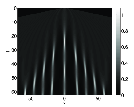
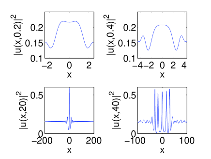
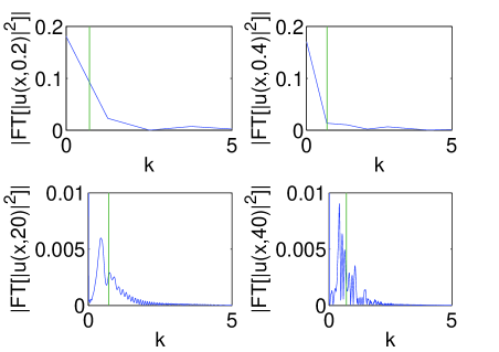
Figure 1: Top panel: Space-time evolution plot of the field intensity (square modulus) $|u|^{2}$ for an initial condition with $u_{0}=0.5$ and a perturbation of $0.05\cos(2{\pi}x)$. Bottom left panels: Four spatial profiles at times $t=0.2$ (stable), $t=0.4$ (marginal), $t=20$ (unstable) and $t=40$ (unstable). Bottom right panels: Four respective Fourier profiles; the smallest wavenumber present in the solution crosses the critical threshold exactly when the domain size equals the critical value, $L_{\rm cr}=2\sqrt{2}\pi$. With time, more subcritical wavenumbers appear and are accordingly amplified.

II.3 Numerical Experiment II: Contracting Domain, No Trap

We now turn to a less orthodox manifestation of MI, which, however, illustrates an important additional dependence of the instability’s critical point, namely the dependence on the amplitude. If, instead of increasing the domain size, we decrease the domain size while increasing background intensity level, so as to maintain the conservation of the $L^{2}$ norm, we also observe a manifestation of MI.

In particular, let us consider a plane wave of amplitude $u_{1}$ in the finite interval $L^{(1)}$. Then, decreasing the interval to $L^{(2)}<L^{(1)}$, while conserving the squared $L^{2}$ norm $\int|u|^{2}dx$, we obtain a plane wave of amplitude $u_{2}$, which is determined by the equation $|u_{1}|^{2}L^{(1)}=|u_{2}|^{2}L^{(2)}$. To this end, utilizing Eq. (4), we readily obtain

$$L_{\rm cr}^{(2)}=L_{\rm cr}^{(1)}\sqrt{\frac{L^{(2)}}{L^{(1)}}}<L_{\rm cr}^{(1)}.$$ (5)

The above result shows that $Q_{\rm cr}^{(2)}>Q_{\rm cr}^{(1)}$, which implies that such a shrinking of the domain (while maintaining conservation of the $L^{2}$ norm) has the potential to result in instability of previously stable modes. In fact, for any $\tilde{L}$, we have a corresponding $\tilde{Q}_{\rm cr}=\tilde{u}\sqrt{2}=u_{1}\sqrt{2L^{(1)}/\tilde{L}}$. So, as the domain size decreases, the critical wavenumber increases, and eventually we expect it to surpass a wavenumber excited in the solution, resulting in MI. This is clearly shown in Fig. 2, which is similar to Fig. 1, but now for a shrinking domain. The dynamical procedure involves linearly decreasing the domain $(-l(t),l(t))$ with a rate $dl/dt=-K$ and preserving the $L^{2}$ norm of the modulus numerically via the rescaling transformation

$$\int_{-l(t)}^{l(t)}|u|^{2}\,dx=\int_{-l_{0}}^{l_{0}}|u|^{2}\,dx.$$ (6)

We observe that in Fourier space it is now the critical point that is shifting to the right, eventually making the configuration unstable, through its crossing of the perturbation wavenumber. The resulting amplification induced by the instability is observed both in the real space formation of large amplitude structures and in the Fourier space growth of the relevant peaks. A noteworthy feature of the top panel of Fig. 2 is that at $t\approx 18$ the middle two localized structures undergo a nearly elastic collision which underscores their solitary wave character.

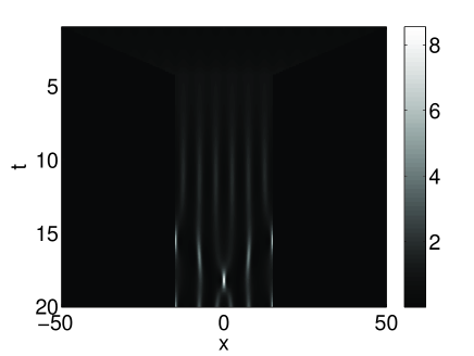
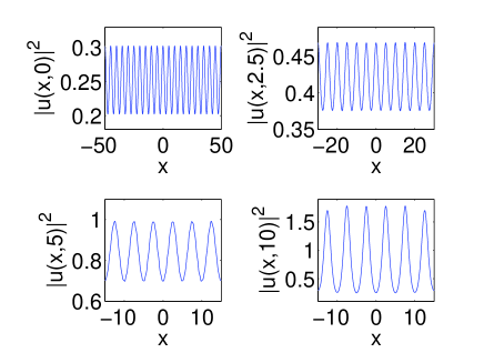
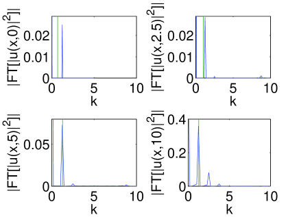
Figure 2: Same as Figure 1, but for the decreasing domain case with fixed $L^{2}$ norm. (Top) The emergence of instability in a space-time intensity plot with decreasing domain size beginning with $l(0)=50$, $K=10$, ${\psi_{0}}=0.5$, and a perturbation of $0.05\cos(2{\pi}x/5)$. Bottom left: Four typical spatial profiles before (upper) and after (bottom) the manifestation of the instability. Bottom right: The four corresponding Fourier profiles are shown, illustrating the emergence of the instability.

II.4 Numerical Experiment III: Expanding Domain, Parabolic Trap

We now turn our attention to the more general inhomogeneous case and consider the full GP equation (1) incorporating the external potential. The latter is known to be particularly relevant to the confinement of the condensate, and assumes typically the harmonic form $V_{\rm ext}(x)=(1/2)\Omega^{2}x^{2}$, as, e.g., in the case of a magnetic or an optical harmonic trap of normalized strength $\Omega$ BEC .

Our motivation for considering this example is the following. For Eq. (1) with the focusing nonlinearity and the parabolic potential, we can obtain the ground state of the system starting, e.g., from the simple linear limit of $g=0$. In that case, Eq. (1) is actually the usual linear Schrödinger equation, which possesses the exact solutions $u(x,t)=\exp(-i\mu t){\psi}(x)$, where $\psi(x)=\exp(-\Omega x^{2}/2\sqrt{2})H_{n}(x)$, where $H_{n}(x)$ is the $n$-th degree Hermite polynomial and $\mu=(2n+1)\Omega/\sqrt{2}$ is the normalized chemical potential. One can then straightforwardly establish (based on continuation arguments), that there is a nonlinear continuation of this linear state bifurcating from the limit of vanishing $L^{2}$ norm (i.e., vanishing number of atoms). This branch of solutions can be obtained with a fixed point algorithm such as a Newton method. There is a unique such continuation for every $n$; see, e.g., kivshar . Here we will consider the ground state, emanating from the solution with $n=0$. For large amplitude, this solution approaches the well-known soliton solution. This is natural since here the nonlinearity tends to focus the solution towards the center of the harmonic trap, where $V_{\rm ext}(x)\rightarrow 0$ and, hence, we revert to the solitonic solution of the untrapped system.

However, for small amplitudes, this ground state branch represents a more extended, nearly-linear solution (i.e., a weakly nonlinear generalization of the linear ground state in the presence of the trap). As such, its width is still critically determined by the trap strength $\Omega$. Therefore, by changing this parameter we may impose on such a nearly-linear solution an effective change in the size of the domain accessible to it. In so doing, we can produce an effectively expanding domain, by virtue of decreasing $\Omega$, or an effectively contracting domain, by means of increasing $\Omega$. These are, respectively, the types of numerical experiments that we will present in this and in the following subsections.

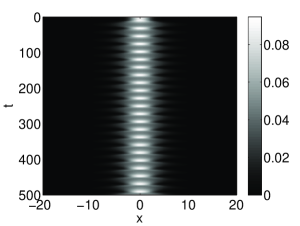
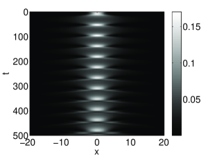
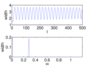
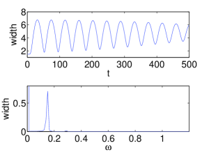
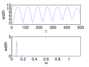
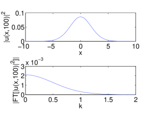
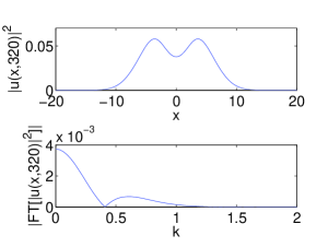
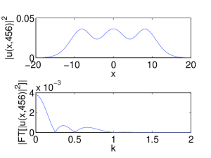
Figure 3: Top row: Intensity space-time contour plots with $\Omega_{1}=0.3$, $\Omega_{2}=0.1$ (left), $\Omega_{2}=0.05$ (middle), and $\Omega_{2}=0.03$ (right). Middle two rows: The corresponding widths as a function of time (upper panels) and frequencies (lower panels). Bottom two rows: Sample spatial profiles (upper panels) and corresponding Fourier profiles (lower panels).

In order to modify the harmonic trap strength, we use a time-dependent parameter $\Omega$, according to

$${\Omega}(t)={\Omega}_{1}+({\Omega}_{2}-{\Omega}_{1})(1+\tanh[(t-t_{0})/{\tau}])/2,$$ (7)

i.e., for $t\ll t_{0}$, the trap strength is $\Omega\approx\Omega_{1}$, for $t\gg t_{0}$, it is $\Omega\approx\Omega_{2}$ (and hence we can expand or shrink the domain, depending on whether $\Omega_{2}<\Omega_{1}$ or $\Omega_{2}>\Omega_{1}$, respectively).

Starting from the case of expanding the domain, we show the relevant results in Figure 3. However, in this version of the problem (i.e., with the parabolic trap), when simply expanding the domain the amplitude of the solution will decrease (rather than being the same as is the case at the boundaries in Experiment I). However, in order to observe the instability, the amplitude of the solution should be preserved. This is achieved by an “injection” of matter in the system, so as to preserve the original amplitude.

This is accomplished in a multiple step process in which we initially integrate until the end of the ramp, at approximately $t^{*}=t_{0}+3\tau$. Next, we calculate the amplitude loss as $a={\rm max}_{x}(|u(0)|)-{\rm max}_{x}(|u(t^{*})|)$. Finally we rerun the simulation, except this time we augment the right hand side of Eq. (1) with a spatially uniform gain rate $\zeta(t)$ over the time when the trap opens up. In particular, the considered modified GP equation and the gain term assume, respectively, the forms:

$$i\partial_{t}u = -\partial_{x}^{2}u+g|u|^{2}u+V_{\rm ext}(x)u+i\zeta(t)u$$ (8)

$$\zeta(t) = \frac{a}{2{\tau}}{\rm sech}^{2}[(t-t_{0})/{\tau}],$$ (9)

which may model the employement of a source of BEC atoms, as in the experiment as . We then observe that if the trap strength is decreased slightly (left set of panels in Fig. 3), the dynamics is going to be stable, in the sense that the distribution of matter will remain unimodal and its width will perform simple small-amplitude oscillations, while the Fourier space profile will remain monotonic (quasi-Gaussian, as the Fourier transform of a near-Gaussian profile in real space). On the other hand, if the trap strength is decreased significantly (middle and right set of panels in Figure 3), then the system becomes “unstable”, in the sense that the spatial profile distribution will become multi-modal (in fact with more humps developing for smaller frequencies), the oscillations of the matter wave width will become more complex (and involve more frequencies) and the Fourier profile will develop nodes, and emergent bands of higher wavenumber excitations, whose number is higher the more multi-modal the spatial distribution becomes.

II.5 Numerical Experiment IV: Contracting Domain, Parabolic Trap

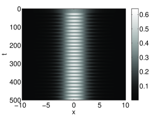
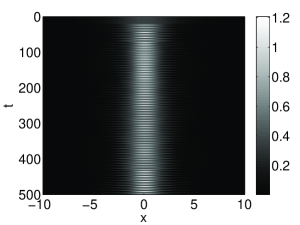
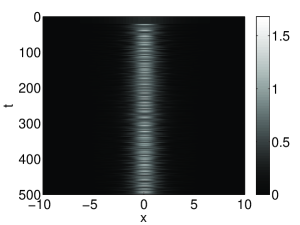
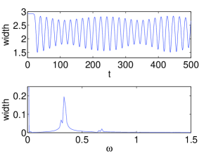
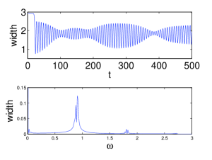
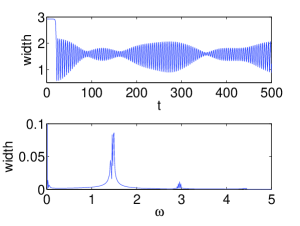
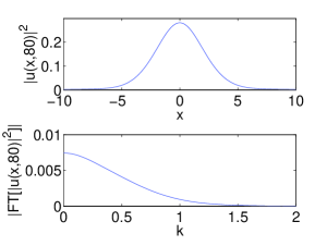
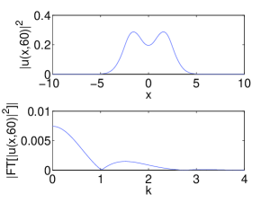
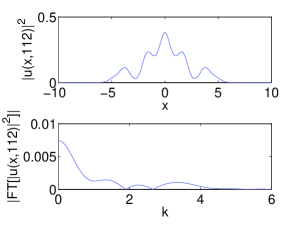
Figure 4: Top row: The full solution intensity space-time contour plots for $\Omega_{1}=0.02$, $\Omega_{2}=0.1$ (left), $\Omega_{2}=0.3$ (middle), and $\Omega_{2}=0.5$ (right). Middle two rows: The corresponding widths as a function of time (upper panels) and frequencies (lower panels). Bottom two rows: Sample spatial profiles (upper panels) and corresponding Fourier profiles (lower panels).

Finally, we consider the case where the strength of the harmonic trap is increased for the same type of solutions as in Numerical Experiment III. Here, the intensity of the solution is increased as the domain is contracting and, hence we can simply allow the dynamics to evolve for different values of $\Omega_{2}>\Omega_{1}$. What we observe suggests a similar scenario of “stability” versus “instability” as in case III. In particular, for small increase of $\Omega$ (left panels of Fig. 4), the dynamics of the spatial profile remains unimodal (and its Fourier transform near-Gaussian) and the beam width oscillates in a near-periodic fashion. On the other hand, for larger trapping strengths (middle and right panels of Fig. 4), the intensity profile involves an increasing number of modes (and its Fourier transform accordingly has multiple nodes), and the oscillation of the beam width becomes increasingly irregular, involving a much wider band of frequencies. Notice that in this case, similar to case II, no injection of matter is necessary: the instability emerges due to the increase in the intensity, necessitated by the conservation of the $L^{2}$ norm.

III Conclusions

In this work, we have explored how the use of the domain size variations and their effects on instabilities can be introduced in a conservative wave setting, by examining the prototypical case of the one-dimensional nonlinear Schrödinger equation. We illustrated that this generic model has a modulational instability that can play a role similar to the Turing instability of reaction-diffusion systems. In particular, we demonstrated that one can take advantage of domain width variability to controllably “excite” the instability and lead to the formation of soliton train patterns in the dispersive system. We examined four different manifestations of this feature. Two of them were relevant to the uniform, untrapped system and two were associated with the setting of an harmonic trap, relevant to Bose-Einstein condensates. In the arguably most standard illustration of the relevant phenomenology (in comparison with its dissipative analog), expansion of a domain for a uniform, untrapped solution led to the realization of a “soliton sprinkler”, emitting more solitons as the domain grew wider. On the other hand, somewhat counter-intuitively, we showed that the instability can even emerge for untrapped systems in contracting domains, provided that the “mass” ($L^{2}$ norm) of the profile is preserved. We also demonstrated how the relevant stability or instability notions can be re-interpreted in the more realistic, yet not spatially uniform, context of harmonically confined condensates. In particular, in the “stable” case, the distribution remained unimodal featuring near-periodic oscillations of its width, while in the “unstable” case, multiple humps emerged in the dynamics of the intensity and complex oscillations in its moments. This was illustrated both for the expanding domain case of decreasing the parabolic trap strength, as well as for the contracting domain case of increasing it.

It would certainly be relevant to implement similar ideas in higher-dimensional settings, where there also exists the additional complication of focusing and wave collapse sulem . It would be especially interesting to elucidate the interplay of the different mechanisms, with the modulational instability inducing the emergence of localized waveforms, which, in turn, may be subject to collapse. It may also be intriguing to implement such ideas in discrete systems, given their recent extensive experimental relevance augusto ; dnc0 and some of the unique features that they possess such as the instability being accessible even for defocusing nonlinearities. Such studies are currently in progress and will be reported in future publications.

Acknowledgements. P.G.K. gratefully acknowledges the support by NSF through the grants DMS-0204585, DMS-CAREER, DMS-0505663 and DMS-0619492. Work at Los Alamos is supported by the US DoE.

References

- (1) E.J Crampin, E.A. Gaffney, P.K.Maini, Bull. of Math. Biol. 61 (1999) 1093.
- (2) E.J. Crampin, W.W. Hackborn, P.K. Maini, Bull. of Math. Biol. 64 (2002) 747.
- (3) E. Crampin, E. Gaffney, P.K. Maini, J. Math. Biol. 44 (2002) 107.
- (4) D.L. Benson, P.K. Maini, J.A. Sherratt, J. Math. Biol. 37 (1998) 381.
- (5) J.D. Murray, Mathematical Biology, Springer-Verlag, Berlin, 2002.
- (6) A. M. Turing, Philos. Trans. R. Soc. Lond. 237 (1952) 37.
- (7) E.J. Crampin, DPhil Thesis, available at: http://www.bioeng.auckland.ac.nz/people/crampin/publications.html
- (8) C. Sulem and P.L. Sulem, The Nonlinear Schrödinger Equation, Springer-Verlag, New York, 1999.
- (9) P.G. Kevrekidis and D.J. Frantzeskakis, Mod. Phys. Lett. B 18 (2004) 173.
- (10) A. Hasegawa and Y. Kodama, Solitons in optical communications, Oxford University Press, New York, 1995.
- (11) L.P. Pitaevskii and S. Stringari, Bose-Einstein Condensation, Clarendon Press, Oxford, 2003.
- (12) E. Infeld and G. Rowlands, Nonlinear Waves, Solitons, and Chaos, Cambridge University Press, Cambridge, 2000. Nonlinear Waves, Solitons, and Chaos, Cambridge University Press (Cambridge, 2000).
- (13) K.S. Strecker, G.B. Partridge, A.G. Truscott, and R.G Hulet, Nature 417 (2002) 150.
- (14) A. Smerzi, A. Trombettoni, P. G. Kevrekidis, and A. R. Bishop, Phys. Rev. Lett. 89 (2002) 170402; F.S. Cataliotti, L. Fallani, F. Ferlaino, C. Fort, P. Maddaloni and M. Inguscio, New J. Phys. 5 (2003) 71.
- (15) J. Meier, G. I. Stegeman, D. N. Christodoulides, Y. Silberberg, R. Morandotti, H. Yang, G. Salamo, M. Sorel, and J. S. Aitchison, Phys. Rev. Lett. 92 (2004) 163902.
- (16) M. Centurion, M.A. Porter, Y. Pu, P.G. Kevrekidis, D.J. Frantzeskakis, D. Psaltis, Phys. Rev. Lett. 97 (2006) 234101; Phys. Rev. A 75 (2007) 063804.
- (17) Yu.S. Kivshar, T.J. Alexander and S.K. Turitsyn, Phys. Lett. A 278 (2001) 225; P.G. Kevrekidis, V.V. Konotop, A. Rodrigues, and D.J. Frantzeskakis, J. Phys. B: At. Mol. Opt. Phys. 38 (2005) 1173.
- (18) A.P. Chikkatur, Y. Shin, A.E. Leanhardt, D. Kielpinski, E. Tsikata, T.L. Gustavson, D.E. Pritchard, and W. Ketterle, Science 296 (2002) 2193.