The Geometric Phase in Supersymmetric Quantum Mechanics

Abstract:

We explore the geometric phase in ${\cal N}=(2,2)$ supersymmetric quantum mechanics. The Witten index ensures the existence of degenerate ground states, resulting in a non-Abelian Berry connection. We exhibit a non-renormalization theorem which prohibits the connection from receiving perturbative corrections. However, we show that it does receive corrections from BPS instantons. We compute the one-instanton contribution to the Berry connection for the massive ${\bf CP}^{1}$ sigma-model as the potential is varied. This system has two ground states and the associated Berry connection is the smooth $SU(2)$ ’t Hooft-Polyakov monopole.

1 Introduction

The purpose of this paper is to explore the geometric phase — or Berry’s phase — among the ground states of quantum mechanical systems exhibiting ${\cal N}=(2,2)$ supersymmetry. Our goal is to show that Berry’s phase and supersymmetry are natural bedfellows: the Berry connection is protected by a perturbative non-renormalization theorem, but receives corrections from BPS instantons.

Berry’s phase governs the evolution of a quantum state as the parameters of the system are varied adiabatically [2, 3, 4]. Consider a Hamiltonian $H(\vec{m})$ depending on the collection of parameters $\vec{m}\in{\cal M}$. We focus on the fate of the $N$ ground states of the system, spanned by the basis $|\psi_{a}(\vec{m})\rangle$, $a=1,\ldots,N$. As the parameters vary adiabatically along a closed path $\Gamma$ in ${\cal M}$, the ground states return to themselves up to a $U(N)$ rotation,

$$|\,\psi_{a}\rangle\rightarrow P\,\exp\left(-i\oint_{\Gamma}\vec{A}_{ab}\cdot d\vec{m}\right)\,|\,\psi_{b}\rangle$$ (1.1)

where the $u(N)$ valued Berry connection over ${\cal M}$ is defined by

$$\vec{A}_{ab}=i\langle\psi_{b}|\frac{\partial}{\partial\vec{m}}|\,\psi_{a}\rangle\ .$$ (1.2)

The canonical example of an Abelian Berry’s phase arises for a spin 1/2 particle in a magnetic field $\vec{B}$

$$H=\vec{B}\cdot\vec{\sigma}$$ (1.3)

where $\vec{\sigma}$ are the Pauli matrices and the magnetic field $\vec{B}\in{\bf R}^{3}$ plays the role of the parameters $\vec{m}$. It is a simple matter to compute the Abelian Berry connection $\vec{A}$ for the ground state of this system [2]: it is the connection of a Dirac monopole, with field strength

$$\vec{\nabla}\times\vec{A}=\frac{\vec{B}}{2B^{3}}$$ (1.4)

The curvature singularity at $\vec{B}=0$ reflects the fact that the spin-up and spin-down states become degenerate at this point. Indeed, the Dirac monopole provides a good approximation to Berry’s phase in the vicinity of any two-state level crossing. However, in more complicated quantum mechanical systems, far from the degenerate point, it is typically difficult to compute the Berry connection since exact expressions for the ground states appearing in (1.2) are rarely known. In this paper we shall show that the Berry connection is exactly computable in quantum mechanical systems with ${\cal N}=(2,2)$ supersymmetry.

The parameters that we will focus on are a triplet of masses $\vec{m}=(m_{1},m_{2},m_{3})$ that exist in supersymmetric quantum mechanics. ${\cal N}=(2,2)$ supersymmetry can be thought of as the dimensional reduction of ${\cal N}=1$ supersymmetry in four dimensions, and the masses $\vec{m}$ arise as background values for the spatial components of the four-dimensional gauge field. The fact that the masses $\vec{m}$ parameterize ${\bf R}^{3}$, just like the magnetic fields of the simple Hamiltonian (1.3), is no coincidence: the Berry connections that we will find will be variants on the theme of the monopole.

The paper is organized as follows. In Section 2, we describe some general properties of ${\cal N}=(2,2)$ quantum mechanics, including the multiplet structure, Lagrangians, symmetries and the space of parameters. Sections 3 and 4 contain the computations of Berry’s phase. Section 3 deals with systems with a single ground state. We present a non-renormalization theorem, previously derived by Denef [9], which protects Berry’s phase from receiving perturbative corrections. This allows us to find exact expressions for Berry’s phase in complicated systems, far from level crossing points. In each case, the Berry connection is simply a sum of Dirac monopoles.

In Section 4 we turn to the more interesting situation with $N>1$ ground states and study the corresponding $U(N)$ Berry connection [4]. The Witten index of supersymmetric systems [10] provides a natural mechanism to ensure the degeneracy of ground states over the full range of parameters. This mechanism is qualitatively different from the coset construction [4] or Kramers degeneracy [11] that has previously been used in the study of non-Abelian Berry’s phase and, in recent years, has found application in condensed matter systems [12, 13, 14] and quantum computing [15, 16]. Our focus will be on the simplest supersymmetric system admitting two ground states: the ${\bf CP}^{1}$ sigma-model with potential governed by $\vec{m}\in{\bf R}^{3}$. We show that BPS instantons carry the right fermi zero-mode structure to contribute to the off-diagonal components of the non-Abelian Berry connection, and we perform the explicit one-instanton calculation. One of the interesting features of this calculation is that, despite supersymmetry, the non-zero modes around the background of the instanton do not cancel. We show that the Berry connection for the ${\bf CP}^{1}$ sigma-model is the $SU(2)$ ’t Hooft-Polyakov monopole which, at large distances, looks like a Dirac monopole, but with the singularity at the origin resolved by instanton effects.

The literature contains a few earlier discussions of the relationship between Berry’s phase and supersymmetry. The $tt^{\star}$ equations of [17, 18, 19] apply in the context of ${\cal N}=(2,2)$ quantum mechanics, and deal with the Berry connection as the complex parameters of the superpotential are varied. This is in contrast to the present paper where we vary the triplet of vector multiplet parameters. The difference is somewhat analogous to the distinction between the Coulomb branch and Higgs branch in higher-dimensional theories and we shall make this analogy more complete in Section 2.1. A discussion of Berry’s phase that is more closely related to the present paper appeared in the context of the matrix theory description of a D2-brane moving in the background of a D4-brane [20]. The calculation of [20] is essentially identical to that of Section 3.1. In a companion paper [21] we will describe a somewhat different non-Abelian Berry’s phase that occurs for a D0-brane moving in the background of a D4-brane.

Note Added: Several aspects discussed in this paper have been clarified in later work. In [22], we showed that the the exact non-Abelian Berry connection discussed in Section 4 is the BPS ’t Hooft-Polyakov monopole. Moreover, in [23] we showed that the Berry phase that arises from varying vector multiplet parameters always solves the Bogomolnyi monopole equations.

2 Supersymmetric Quantum Mechanics

Quantum mechanics with ${\cal N}=(2,2)$ supersymmetry follows from the dimensional reduction of ${\cal N}=1$ supersymmetric theories in four dimensions. The superalgebra has four real supercharges and is sometimes referred to as $N=4A$ supersymmetry. The supercharges form a complex doublet $Q_{\alpha}=(Q_{-},Q_{+})$ with the supersymmetry algebra given by,

$$\{Q_{\alpha},Q_{\beta}\}=\{\bar{Q}_{\alpha},\bar{Q}_{\beta}\}=0\ \ \ ,\ \ \ \{Q_{\alpha},\bar{Q}_{\beta}\}=2H\delta_{\alpha\beta}+2\vec{\sigma}_{\alpha\beta}\cdot\vec{Z}$$ (2.5)

The triplet of central terms $\vec{Z}$ can be thought of as the momentum in the three reduced dimensions. The automorphism group of the algebra is

$$R=SU(2)_{R}\times U(1)_{R}\ ,$$ (2.6)

under which the supercharges $Q$ transform in the ${\bf 2}_{\,+\!1}$ representation, while the central charges $\vec{Z}$ transform as ${\bf 3}_{\,0}$. We start with a brief review of the different supersymmetric multiplets that we will make use of; for the most part these are familiar from other theories with four supercharges.

Vector and Linear Multiplets

The Abelian vector multiplet $V$ contains a single gauge field $A_{0}$. In quantum mechanics its role is to impose the constraint of Gauss’ law on the Hilbert space. The propagating degrees of freedom consist of three real scalars $\vec{X}$ that arise from the dimensional reduction of the four-dimensional gauge field, and a pair of complex fermions $\lambda_{\pm}$. There is also an auxiliary field $D$. Under the R-symmetry, $\vec{X}$ transforms in ${\bf 3}_{\,0}$ while $\lambda$ transforms in ${\bf 2}_{\,+1}$. We will usually write $\lambda=(\lambda_{-},\lambda_{+})^{T}$.

In higher-dimensional theories, it is useful to consider the gauge-invariant multiplet, which contains the Abelian field strength as opposed to the gauge potential. In quantum mechanics, the analogous object is a triplet of linear multiplets $\vec{\Sigma}$ [24, 25],

$$\vec{\Sigma}=\frac{1}{2}\bar{D}\vec{\sigma}DV=-\vec{X}+i{\theta}\vec{\sigma}\bar{\lambda}+i\bar{\theta}\vec{\sigma}\lambda-\bar{\theta}\vec{\sigma}\theta D+\bar{\theta}(\vec{\sigma}\times\,\dot{\!\!\vec{X}}\,)\theta+\ldots$$

The kinetic terms for the vector multiplet are given by

$$L_{vector}=\frac{1}{g^{2}}\int d^{2}\theta d^{2}\bar{\theta}\ \vec{\Sigma}^{2}=\frac{1}{2g^{2}}\ \dot{\!\!\vec{X}}{}^{2}+\frac{i}{g^{2}}\bar{\lambda}\dot{\lambda}+\frac{1}{2g^{2}}D^{2}$$ (2.7)

In non-relativistic quantum mechanics, the coefficient $1/g^{2}$ should be thought of as the mass of a particle moving in the $\vec{X}$ direction; nonetheless we continue to use the notation of coupling constants more appropriate to higher dimensional field theories.

Chiral Multiplets

The chiral multiplet $\Phi$ is familiar from four dimensions and so we will be brief. It contains a complex scalar $\phi$ and a pair of complex Grassmann fields $\psi_{\pm}$ which we again write as $\psi=(\psi_{-},\psi_{+})^{T}$. There is also the complex auxiliary field $F$. The scalars $\phi$ are invariant under $SU(2)_{R}$, while the fermions are doublets. For a chiral multiplet with charge $q$ under the $U(1)$ vector multiplet, the Lagrangian is given by

$$L_{\rm chiral} = \int d^{2}\theta d^{2}\bar{\theta}\ \bar{\Phi}\,e^{2qV}\Phi$$

$$= |{\cal D}_{t}\phi|^{2}+\bar{\psi}(i{\cal D}_{t}-\vec{X}\cdot\vec{\sigma})\psi+|F|^{2}+qD|\phi|^{2}-q^{2}\vec{X}^{2}|\phi|^{2}-i\sqrt{2}q(\bar{\phi}\epsilon_{\alpha\beta}\psi_{\alpha}\lambda_{\beta}-{\rm h.c.})$$

with ${\cal D}_{t}\phi=\dot{\phi}-iqA_{0}\phi$. In this paper we will work with Abelian gauged linear sigma models [26], built from a single $U(1)$ vector multiplet coupled to some number of chiral multiplets.

2.1 The Parameter Space

The Berry connection is a gauge connection over the space of parameters ${\cal M}$ of the theory. Supersymmetric quantum mechanics has a number of different parameters, which can be considered as background fields living in different supermultiplets.

As is familiar from many contexts, complex parameters that appear in the superpotential lie in background chiral multiplets. Just as in higher-dimensional field theories [27], certain properties of the quantum mechanics depend analytically on these parameters. For example, this holomorphic dependence is behind the $tt^{\star}$ equations of [17]. We can introduce a complex mass parameter $\mu$ of this type only if we have two chiral multiplets, $\Phi$ and $\tilde{\Phi}$, carrying opposite gauge charge. We can then write the gauge-invariant superpotential,

$${\cal W}=\mu\,\tilde{\Phi}\Phi$$ (2.9)

A second class of parameters lives in the linear multiplets $\vec{\Sigma}$. These are the triplet of mass parameters described in the introduction. They are associated to weakly gauging a $U(1)_{F}$ flavour symmetry of the quantum mechanics and, unlike the complex mass parameter $\mu$, can be assigned to a single chiral multiplet $\Phi$,

$$L_{\rm mass}=\int d^{4}\theta\,\Phi^{\dagger}\exp\left(\bar{\theta}\,\vec{m}\cdot\vec{\sigma}\,\theta\right)\Phi=|\dot{\phi}|^{2}+i\bar{\psi}\dot{\psi}-m^{2}\,|\phi|^{2}-\bar{\psi}(\vec{m}\cdot\vec{\sigma})\psi$$ (2.10)

Here $m=|\vec{m}|$. If $\Phi$ also carries charge $q$ under the $U(1)$ gauge multiplet, the mass terms are given by $(q\vec{X}-\vec{m})^{2}|\phi|^{2}$, with similar expressions for the fermions.

An important feature of these parameters is that it may not be consistent with supersymmetry to turn on $\mu\neq 0$ and $\vec{m}\neq 0$ at the same time. This can be most simply seen by viewing $\vec{m}$ and $\mu$ as dynamical background supermultiplets. To illustrate this, consider the theory with two chiral multiplets $\Phi$ and $\tilde{\Phi}$ of gauge charge $+1$ and $-1$ respectively. One may introduce a triplet of masses $\vec{m}$ by weakly gauging the $U(1)_{F}$ global symmetry under which both $\Phi$ and $\tilde{\Phi}$ have charge $+1$. This will give rise to masses,

$$(\vec{X}-\vec{m})^{2}|\phi|^{2}+(\vec{X}+\vec{m})^{2}|\tilde{\phi}|^{2}$$ (2.11)

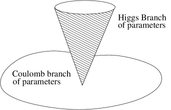
Figure 1: The parameter space of the supersymmetric quantum mechanics.

However, invariance of the superpotential (2.9) under $U(1)_{F}$ requires that $\mu$ carries charge $-2$. This results in the further contribution to the potential energy $4m^{2}\,|\mu|^{2}$ which gives a non-zero ground-state energy, and hence breaks supersymmetry, if both $\vec{m}$ and $\mu$ are non-vanishing. This kind of behaviour is very familiar for dynamical fields where it gives rise to the usual distinction between the Coulomb branch and Higgs branch of vacua. Here we see the same phenomenon at play in the space of parameters, rather than the space of vacua. We use the same nomenclature. The space of parameters of the theory is depicted in the figure: $\mu$ provides a coordinate for the Higgs branch of parameters, while $\vec{m}$ provide coordinates on the Coulomb branch. In this paper, we will focus on the Berry connection over the Coulomb branch of parameters.

There are two further parameters of interest. We have already seen the gauge coupling constant $g^{2}$ in the vector multiplet Lagrangian. We may also introduce a real Fayet Iliopoulos (FI) parameter $r$ by the $SU(2)_{R}$ invariant integral,

$$L_{FI}=r\int d\bar{\theta}\,\vec{\sigma}\,d\theta\cdot\vec{\Sigma}=rD$$ (2.12)

3 Abelian Berry’s Phase

In this section we discuss Berry’s phase in systems with a single ground state. We start with the simplest occurrence of Berry’s phase: a free chiral multiplet $\Phi$ with the mass triplet $\vec{m}$. Since this will provide the “tree-level” approximation to Berry’s phase in more complicated systems, we spend some time describing this basic set-up from both the Hamiltonian and the Lagrangian viewpoints. The latter will provide a useful spring-board to discuss Berry’s phase in interacting theories.

3.1 Berry’s Phase in a Free Theory

Using the spinor notation $\psi^{T}=(\psi_{-},\psi_{+})$, the Lagrangian for a free chiral multiplet $\Phi$ with mass $\vec{m}$ is,

$$L_{\rm free}=|\dot{\phi}|^{2}+i\bar{\psi}\dot{\psi}-m^{2}\,|\phi|^{2}-\bar{\psi}(\vec{m}\cdot\vec{\sigma})\psi\ .$$ (3.13)

Note that the fermion mass term is reminiscent of the simple Hamiltonian (1.3) described in the introduction. This term will indeed be responsible for Berry’s phase.

We pass to the Hamiltonian formalism by introducing the canonical momenta $\pi=\dot{\phi}^{\dagger}$ and the Fermionic conjugate momenta $\partial L/\partial\dot{\psi}=-i\bar{\psi}$, giving us a Hamiltonian consisting of a two bosonic and two fermionic harmonic oscillators,

$$H=|\pi|^{2}+\vec{m}^{2}|\phi|^{2}+\bar{\psi}(\vec{m}\cdot\vec{\sigma})\psi$$ (3.14)

We now quantize this theory using the canonical approach. We use the usual Schrödinger representation for the bosonic fields,

$$[\phi,\pi]=i\ \ \ \Rightarrow\ \ \ \pi=-i\frac{\partial}{\partial\phi}$$ (3.15)

while the fermionic anti-commutation relations $\{\psi,\bar{\psi}\}=1$ are implemented by defining a reference state $|\,0\rangle$ annihilated by $\psi$: $\psi_{+}|\,0\rangle=\psi_{-}|\,0\rangle=0$. We then form a basis of the fermionic Hilbert space by acting on $|\,0\rangle$ with the creation operators $\bar{\psi}_{\pm}$ to form the four states,

$$|\,0\rangle\ \ ,\ \ \bar{\psi}_{+}|\,0\rangle\ \ \,\ \ \bar{\psi}_{-}|\,0\rangle\ \ ,\ \ \bar{\psi}_{+}\bar{\psi}_{-}|\,0\rangle$$ (3.16)

We focus on the fermionic part of the Hamiltonian,

$$H_{F}=\bar{\psi}(\vec{m}\cdot\vec{\sigma})\psi$$ (3.17)

The top and bottom states are both excited states in the Hilbert space: they have $H_{F}|\,0\rangle=H_{F}\,\bar{\psi}_{+}\bar{\psi}_{-}|\,0\rangle=0$ so that, once dressed with the ground state of the complex boson $\phi$, they have energy $+m$. Here we focus on the ground state of the system which lies in the two-dimensional fermionic Hilbert space ${\cal H}_{2}$ spanned by $\bar{\psi}_{\pm}|\,0\rangle$. The fermionic Hamiltonian (3.17) acts on this space as,

$$H_{F}=\vec{m}\cdot\vec{\sigma}$$ (3.18)

$H_{F}$ has eigenvalues $\pm m$. The fermionic ground state $|\,\Omega\rangle$ satisfies $H_{F}|\,\Omega\rangle=-m|\,\Omega\rangle$ so that, once dressed with the bosonic ground state, it yields a state with vanishing energy as expected in a supersymmetric system.

The Hamiltonian (3.18) acting on the ground state coincides with that of a spin 1/2 particle in a magnetic field (1.3). Correspondingly, the Berry connection of the ground state as the parameters $\vec{m}$ are varied is given by the Dirac monopole. To give an explicit form of the connection, we should first pick a gauge which, in this context, means reference choice of ground state — including the phase — for each $\vec{m}$. To this end, we define the projection operator onto the ground state

$$P_{-}=\frac{1}{2}\left({\bf 1}-\frac{\vec{m}}{m}\cdot\vec{\sigma}\right)$$ (3.19)

Then we define the phase of our reference ground states to be that of the (un-normalized) state $P_{-}\,\bar{\psi}_{+}|\,0\rangle$, which is valid everywhere except along the half-line $\vec{m}=(0,0,-m)$ where the ground state $|\Omega\rangle$ is orthogonal to $\bar{\psi}_{+}|\,0\rangle$. As a result, the Berry connection has a Dirac string singularity along this axis. The Berry connection is $\vec{A}=i\langle\Omega|\vec{\nabla}|\Omega\rangle$. It is a simple matter to compute the explicit connection which is given by the Dirac monopole. In Cartesian coordinates, it is

$$A^{\rm Dirac}_{i}=\frac{\epsilon_{ij}m_{j}}{2m(m+m_{3})}\ \ \ {i,j=1,2}\ \ \ {\rm and}\ \ \ A^{\rm Dirac}_{3}=0$$ (3.20)

For a closed, adiabatic variation of the parameters $\vec{m}$, the Berry phase is the then given by the integral of this connection so that

$$|\,\Omega\rangle\rightarrow\exp\left(-i\oint\vec{A}\cdot d\vec{m}\right)|\,\Omega\rangle$$ (3.21)

3.2 The Born-Oppenheimer Approximation

One man’s fixed parameter is another’s dynamical degree of freedom. This is the essence of the Born-Oppenheimer approximation in which the “parameters” of the model are not really fixed, but merely slowly moving degrees of freedom. We may endow the parameters $\vec{m}$ with dynamics by introducing the canonical kinetic terms

$$L_{m}=\frac{1}{2e^{2}}\,\dot{\vec{m}}{}^{2}$$ (3.22)

The Born-Oppenheimer approximation is then valid if $e^{2}\ll\langle m\rangle^{3}$. This ensures that the $\phi$ fields have high frequency and may be treated in a fixed $\vec{m}$ background. From a modern perspective, this is equivalent to the Wilsonian approach to quantum mechanics, in which the fast moving $\phi$ degrees of freedom are integrated out. (Note, however, that in quantum mechanics the fast moving degrees of freedom are the physical light particles, while in field theory they are the virtual heavy particles). As in field theory, the Born-Oppenheimer-Wilson framework is ideally suited to working in the language of path integrals and effective actions rather than Hamiltonians [28, 29]. In this section we show how to reproduce the Berry’s phase from this perspective.

We wish to integrate out the $\phi$ and $\psi$ fields in (3.13) in the background of time varying parameters $\vec{m}(t)$. This results in contributions to the effective action for $\vec{m}$. The contribution from the bosons $\phi$ is given by

$${\cal L}_{\rm bose}=\log\det\left(\frac{-\partial_{t}^{2}-m(t)^{2}}{-\partial_{t}^{2}-{m}_{0}^{2}}\right)$$ (3.23)

where the vacuum value for the masses may be taken to be $\vec{m}_{0}=\frac{1}{T}\int_{0}^{T}dt\,\vec{m}(t)$. The determinant may be easily computed as an expansion of $\dot{\vec{m}}$. The first two terms are given by

$${\cal L}_{\rm bose}=-m+\frac{\dot{\vec{m}}{}^{2}}{8m^{3}}+\ldots$$ (3.24)

Here the first term corresponds to the usual zero-point energy of $\phi$, while the second term can be interpreted as a finite renormalization of the kinetic term $1/e^{2}\rightarrow 1/e^{2}+1/4m^{3}$.

The contribution from the fermions $\psi$ is given by the determinants

$${\cal L}_{\rm fermi}=-\log\det\left(\frac{i\partial_{t}-\vec{m}(t)\cdot\vec{\sigma}}{i\partial_{t}-\vec{m}_{0}\cdot\vec{\sigma}}\right)$$ (3.25)

These determinants include the Berry phase, as first shown by Stone [30]. The simplest way to see this is to recall that the determinants compute the vacuum-vacuum amplitude. To leading order, this includes the dynamical phase $e^{i\int dt\,m(t)}$ and the Berry phase $e^{i\int dt\,\vec{A}\cdot\dot{\vec{m}}}$. This translates into an effective action,

$${\cal L}_{\rm fermi}=+m+\vec{A}(\vec{m})\cdot\dot{\vec{m}}+\ldots$$ (3.26)

The first term is the zero point energy of a Grassmannian variable and cancels the contribution in (3.24) as expected in a supersymmetric theory. The Berry connection appearing in the second term is the Dirac monopole (3.20). There is no further renormalization to the kinetic terms from the fermions. In summary, the effect of these simple one-loop computations in quantum mechanics is to provide an effective low-energy dynamics of the parameters $\vec{m}$ which, up to two derivatives, is given by

$$L_{\rm eff}=\vec{A}\cdot\dot{\vec{m}}+\left(\frac{1}{2e^{2}}+\frac{1}{8m^{3}}\right)\dot{\vec{m}}{}^{2}+\ldots$$ (3.27)

with the first term identified as the Berry connection.

The Supersymmetric Completion

As we reviewed in Section 2.1, the parameters $\vec{m}$ can be thought of as living in a supersymmetric vector multiplet $V$. As well as the three parameters $\vec{m}$, this multiplet also contains a gauge field $u$, an auxiliary scalar $D$ and two complex fermions $\eta_{\pm}$. If we are to apply the Born-Oppenheimer approximation in a supersymmetric manner, the kinetic terms (3.22) must be accompanied with suitable terms for the other fields in the multiplet, together with further Yukawa coupling interactions. For $e^{2}\neq 0$, the Lagrangian (3.22) should be replaced by,

$$L_{m} = \frac{1}{2e^{2}}\dot{\vec{m}}{}^{2}+\frac{i}{e^{2}}\bar{\eta}\dot{\eta}+\frac{1}{2e^{2}}D^{2}$$ (3.28)

while (3.13) is now generalized to include interaction terms between the chiral multiplet and vector multiplet fields, given by (2) with $\vec{X}$ replaced by the parameter $\vec{m}$, and $\lambda$ replaced by $\eta$. In the Born-Oppenheimer approximation, we once again should integrate out the chiral multiplet in the regime $e^{2}\ll\langle m\rangle^{3}$. We now search for an effective action for the vector multiplet that itself preserves supersymmetry. Such an action was derived by Denef in [9]. (As action of the same form was also derived previously by Smilga in the study of the zero mode dynamics of SQED [31, 32]. Integrating out the chiral multiplets gives the supersymmetric completion of the Berry term,

$${\cal L}_{\rm Berry}=\vec{A}\cdot\dot{\vec{m}}-\frac{1}{2m}D+\bar{\eta}\,\frac{\vec{m}\cdot\vec{\sigma}}{2m^{3}}\eta$$ (3.29)

This Lagrangian is invariant under the supersymmetry transformations,

$$\delta u = i\bar{\eta}\xi-i\bar{\xi}\eta$$

$$\delta\vec{m} = i\bar{\eta}\vec{\sigma}\xi-i\bar{\xi}\vec{\sigma}\eta$$ (3.30)

$$\delta\eta = \dot{\vec{m}}\cdot\vec{\sigma}\xi+iD\xi$$

$$\delta D = -\dot{\bar{\eta}}\xi-\bar{\xi}\dot{\eta}$$

One of the consequences of supersymmetry is that the presence of kinetic terms for parameters also introduces new interaction terms. These are written in equation (2) and they further affect the dynamics of the theory. For example, the D-term interactions in (2) give rise to a one-loop potential over the parameter space. This is then captured in the effective theory (3.29) by the D-term which gives rise to the potential,

$$V=\frac{1}{8m^{2}}\left(\frac{1}{e^{2}}+\frac{1}{4m^{3}}\right)^{-1}$$ (3.31)

where we have invoked the coupling renormalization (3.27). Thus the true supersymmetric vacuum lies at $m\rightarrow\infty$. One may wonder whether these interactions also change the Berry connection, which was computed in the strict $e^{2}=0$ limit. In principle there could be $e^{2}/m^{3}$ corrections to the connection. The fact that this cannot happen follows from a non-renormalization theorem proven by Denef [9]. He considered the most general Lagrangian containing a single time derivative and fermi bi-linear terms, consistent with the $SU(2)_{R}$ symmetry of the model,

$${\cal L}=\vec{A}(\vec{m})\cdot\dot{\vec{m}}-U(m)D+C(m)\bar{\eta}\eta+\bar{\eta}\,\vec{C}(\vec{m})\cdot\vec{\sigma}\eta$$ (3.32)

with arbitrary functions $\vec{A}$, $U$, $C$ and $\vec{C}$. Requiring that this action is supersymmetric places strong constraints on these functions. The supersymmetry transformations (3.30) are dictated (at this order) by the superspace formulation [25]. Invariance of the Lagrangian then requires,

$$\vec{C}={\nabla}U={\nabla}\times\vec{A}\ \ \ \ {\rm and}\ \ \ \ C=0$$ (3.33)

Allowing for singular behaviour at the origin, the most general spherically symmetric solution to these constraints is the Dirac monopole connection (3.20). This is the promised non-renormalization theorem for the Berry connection. We will now apply this to compute Berry’s phase in more complicated, interacting theories.

3.3 Berry’s Phase in Interacting Theories

We now turn to interacting theories where more complicated Berry’s connections may be expected. In this section we restrict to theories with a single ground state, ensuring an Abelian Berry connection. We will treat the more interesting theories with multiple, degenerate ground states in the following section.

We consider the $U(1)$ gauge theory with two chiral multiplets $\Phi$ and $\tilde{\Phi}$ of charge $+1$ and $-1$ respectively. This is the dimensional reduction of ${\cal N}=1$ SQED. The bosonic part of the Lagrangian is given by,

$$L=\frac{1}{2g^{2}}\dot{\vec{X}}{}^{2}+|{\cal D}_{t}\phi|^{2}+|{\cal D}_{t}\tilde{\phi}|^{2}-X^{2}(|\phi|^{2}+|\tilde{\phi}|^{2})-\frac{g^{2}}{2}(|\phi|^{2}-|\tilde{\phi}|^{2}-r)^{2}$$ (3.34)

Note that we have introduced a FI parameter $r>0$. Although the vector multiplet scalars $\vec{X}$ look ripe to treat in the Born-Oppenheimer approximation, we will not do so here; instead we take the limit $g^{2}\rightarrow\infty$ where the theory reduces to a gauged linear sigma-model with target space defined by the D-flatness conditions,

$$|\phi|^{2}-|\tilde{\phi}|^{2}=r$$ (3.35)

modulo the gauge action $\phi\rightarrow e^{i\alpha}\phi$ and $\tilde{\phi}\rightarrow e^{-i\alpha}\tilde{\phi}$. Asymptotically this is the cone ${\bf C}/{\bf Z}_{2}$. The conical singularity is resolved by the FI parameter $r>0$. Since we are not treating $\vec{X}$ as the parameters for Berry’s connection, we must introduce different parameters. We will do that now.

The Parameter Space

We wish to introduce a potential on the target space. As discussed in Section 2.1, there is a Higgs branch and Coulomb branch of parameters for this model. The physics on these two branches is very different.

Moving on the Higgs branch of parameters requires us to introduce the gauge invariant superpotential ${\cal W}=\mu\,\tilde{\Phi}\Phi$. When $\mu\neq 0$, there is no simultaneous solution to the D-term constraints (3.35) and the F-term constraints $\phi=\tilde{\phi}=0$, and supersymmetry is spontaneously broken.

Moving on the Coulomb branch of parameters introduces the triplet of masses $\vec{m}$ arising from weakly gauging the $U(1)_{F}$ flavour symmetry of the model, under which $\Phi\rightarrow e^{i\alpha}\Phi$ and $\tilde{\Phi}\rightarrow e^{i\alpha}\tilde{\Phi}$. The masses sit in the Lagrangian by replacing the $X^{2}(|\phi|^{2}+|\tilde{\phi}|^{2})$ term in (3.34) by (2.11). In contrast to the complex mass, the presence of $\vec{m}$ does not break supersymmetry. The theory has a unique classical ground state given by

$$\vec{X}=\vec{m}\ \ \ ,\ \ \ |\phi|^{2}=r\ \ \ ,\ \ \tilde{\phi}=0$$ (3.36)

This behaviour is consistent with the Witten index because the point $\mu=\vec{m}=0$ is singular: here the potential on the non-compact vacuum moduli space vanishes, allowing the ground state wavefunction to spread into the asymptotic regime of ${\bf C}/{\bf Z}_{2}$ and become non-normalizable. At this point, the zero-energy state exits the Hilbert space of the theory and the theory breaks supersymmetry.

Berry’s Phase

On the Coulomb branch of parameters, the dimensionless coupling for our massive sigma model is $1/mr$. For $mr\gg 1$, the ground state wavefunction is restricted to a region of field space much smaller than the curvature of the target space, and is well approximated by the free theory described in Section 3.1. The Berry connection for the ground state is, to leading order, described by the Dirac monopole (3.20). However, we naively expect corrections to the Berry connection, which can be computed perturbatively in $1/mr$, as the ground state wavefunction begins to feel the curvature of the target space. The fact that such corrections cannot occur has nothing to do with the supersymmetric non-renormalization theorem, but instead follows from the fact that the quantized flux emitted from the singularity is conserved as one moves in parameter space. This ensures that any corrections to the curvature are solenoidal in nature. Yet there are no such corrections consistent with the $SO(3)$ rotational symmetry of the problem.

3.3.1 Further Examples

It is a simple matter to cook up related models with a single ground state without $SO(3)$ symmetry. We could consider the gauged linear sigma model built from $U(1)$ with a single chiral multiplet $\Phi$ of charge $+1$ and $M$ chiral multiplets $\tilde{\Phi}_{i}$ of charge $-1$. The D-term constraint is

$$|\phi|^{2}-\sum_{i=1}^{M}|\tilde{\phi}_{i}|^{2}=r$$ (3.37)

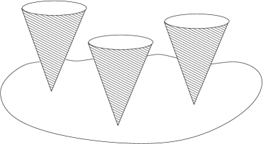
Figure 2: The parameter space with multiple chiral multiplets.

We endow $\Phi$ with the triplet of masses $\vec{m}$, and each $\tilde{\Phi}_{i}$ with masses $\vec{\tilde{m}}_{i}$. For $r>0$ and $\vec{m}\neq\vec{\tilde{m}}_{i}$, the theory has a unique classical ground state given by $\vec{X}=\vec{m}$ and $|\phi|^{2}=r$ with $\tilde{\phi}_{i}=0$. For the present purposes we will fix $\vec{\tilde{m}}_{i}$ and ask about the behaviour of the ground state as we vary $\vec{m}$. We expect $M$ singular points, lying at $\vec{m}=\vec{\tilde{m}}_{i}$, at which a branch of Higgs vacua emerges. Alternatively, we can view these as points where a new Higgs branch of supersymmetric parameters is admitted, corresponding to a superpotential ${\cal W}=\mu_{i}\tilde{\Phi}_{i}\Phi$, so that the parameter space of the theory looks like that shown in Figure 2.

Now the symmetries of the problem are not sufficient to rule out general solenoidal contributions to the Berry connection. However, the non-renormalization theorem of the previous section is: we may integrate out all fields to derive an effective action for the parameters $\vec{m}$ which is of the form (3.32). The constraints (3.33) are now satisfied by a superposition of Dirac monopoles, lying at positions $\vec{m}=\vec{\tilde{m}_{i}}$,

$$\nabla\times\vec{A}=\sum_{i=1}^{M}\frac{\vec{m}-\!\vec{\,\,\tilde{m}_{i}}}{2|\vec{m}-\!\vec{\,\,\tilde{m}_{i}}|^{3}}$$ (3.38)

In summary, the restriction of supersymmetry requires that the Berry’s phase does not receive any corrections from its simple “tree-level” value and, even in the full interacting theory is still given by the Dirac monopole. While it is pleasing to be able to make precise statements about objects in interacting quantum mechanics it is, nonetheless, a little disappointing that the object is not particularly novel. In the next section we will instead turn to a situation where a more interesting Berry connection emerges.

4 Non-Abelian Berry’s Phase

Supersymmetry provides a natural arena in which to study non-Abelian Berry’s phases. Unlike previous examples [4, 11], the the degeneracy of ground states is dictated not by a symmetry, but rather by an index. In this section we discuss a simple supersymmetric system with two ground states. We compute the $U(2)$ Berry connection over the ${\bf R}^{3}$ parameter space. We show that it is given by a smooth ’t Hooft-Polyakov monopole.

4.1 The ${\bf CP}^{1}$ Sigma Model

Our simple model is supersymmetric quantum mechanics with ${\bf CP}^{1}$ target space and a potential. We construct this target space from a gauged linear theory with $U(1)$ gauge group and two chiral multiplets, both of charge $+1$. The bosonic part of the Lagrangian is given by,

$$\ L=\frac{1}{2g^{2}}\dot{\vec{X}}{}^{2}+\sum_{i=1}^{2}|{\cal D}_{t}\phi_{i}|^{2}-(\vec{X}-\vec{m}_{i})^{2}|\phi_{i}|^{2}-\frac{g^{2}}{2}(|\phi_{1}|^{2}+|\phi_{2}|^{2}-r)^{2}$$ (4.39)

In the limit $g^{2}\rightarrow\infty$, the D-term restricts us to ${\bf S}^{3}$ defined by,

$$|\phi_{1}|^{2}+|\phi_{2}|^{2}=r$$ (4.40)

Further dividing by gauge transformations $\phi_{i}\rightarrow e^{i\alpha}\phi_{i}$ leaves us with the target space ${\bf CP}^{1}\cong{\bf S}^{2}$. The triplets of mass parameters $\vec{m}_{i}$ induce a potential on this space. By a suitable shift of $\vec{X}$ we may choose

$$\vec{m}_{1}=-\vec{m}_{2}\equiv\vec{m}$$ (4.41)

We are interested in computing the Berry connection that arises as we adiabatically vary $\vec{m}$. (The ${\bf CP}^{1}$ model was also the system in which the $tt^{\star}$ equations were first applied to compute Berry’s phase, this time as the complexified Kähler class $t=r+i\theta$ of the $d=1+1$ dimensional theory is varied [19]).

In the absence of masses $\vec{m}$, the model admits an $SU(2)_{F}$ global symmetry, transforming $\phi_{i}$ in the doublet representation. This is simply the isometry of the ${\bf CP}^{1}$ target space. The masses can be thought of as living in a background vector multiplet for $SU(2)_{F}$ and therefore transform in the adjoint representation. Since $\vec{m}$ also transforms in the ${\bf 3}$ of $SU(2)_{R}$, it breaks the non-Abelian global symmetries to their Cartan subalgebra

$$\vec{m}:SU(2)_{F}\times SU(2)_{R}\rightarrow U(1)_{F}\times U(1)_{A}$$ (4.42)

The global $U(1)_{F}$ symmetry acts on the bosons as $\phi_{1}\rightarrow e^{i\theta}\phi_{1}$ and $\phi_{2}\rightarrow e^{-i\theta}\phi_{2}$ and will play a role in the discussion of instantons. For non-zero $\vec{m}$, the theory has two, isolated, classical vacua. They are

• Vacuum 1: $\vec{X}=\vec{m}$ with $|\phi_{1}|^{2}=r$ and $\phi_{2}=0$.

• Vacuum 2: $\vec{X}=-\vec{m}$ with $\phi_{1}=0$ and $|\phi_{2}|^{2}=r$.

The Witten index ensures that both of these vacua survive in the quantum theory [10]. This introduces yet another $U(2)_{G}$ symmetry, which is the gauge symmetry rotating these ground states in the quantum theory. This is the reason that our Berry connection is, a priori, a $U(2)$-valued object over ${\bf R}^{3}$. However, in this case there exists a distinguished basis of ground states, given by the eigenstates under $U(1)_{F}$. (In fact, $U(1)_{A}$ would do equally well for these purposes). The fact that the ground states carry different quantum numbers under $U(1)_{F/A}$ leads to “spontaneous breaking” of the $U(2)_{G}$ symmetry to the Cartan subalgebra, which can then be identified with $U(1)_{R}\times U(1)_{F}$. Note that at the origin of parameter space $\vec{m}=0$, there is no breaking (4.42) and, correspondingly, no way to distinguish the two ground states; here $U(2)_{G}$ remains unbroken.

Berry’s Phase

The dimensionless coupling of our model is $1/mr$. In the limit $mr\gg 1$, the physics around each vacuum is described by a single, free chiral multiplet and, to leading order, the ground state is simply Gaussian. In vacuum 1, $\phi_{1}$ is eaten by the Higgs mechanism and the remaining dynamical field is $\Phi_{2}$, with mass $+2\vec{m}$. As explained in Section 3.1, the $U(1)$ Berry’s connection for this vacuum is the Dirac monopole connection $\vec{A}{}^{\rm Dirac}$. In contrast, in vacuum 2 the free chiral multiplet is $\Phi_{1}$ with mass $-2\vec{m}$ and the Berry connection is $-\vec{A}{}^{\rm Dirac}$. Putting these two results together, the leading order $U(2)$ Berry connection is given by

$$\vec{A}=\vec{A}{}^{\rm Dirac}\,\sigma^{3}$$ (4.43)

which, in fact, lies in $SU(2)$ rather than $U(2)$. This connection inherits the Dirac string singularity along the $\vec{m}=(0,0,-m)$ half-axis. However, as is well known, one may eliminate this through the use of a singular $SU(2)$ gauge transformation,

$$U=\exp\left(-\frac{i\theta(m_{2}\sigma^{1}-m_{1}\sigma^{2})}{2\sqrt{m^{2}-m_{3}^{2}}}\right)$$ (4.44)

under which the Dirac monopole-anti-monopole pair (4.43) becomes $\tilde{A}_{\mu}=UA_{\mu}U^{\dagger}-i(\partial_{\mu}U)U^{\dagger}$ which takes the rotationally symmetric form,

$$\tilde{A}_{\mu}=\epsilon_{\mu\nu\rho}\,\frac{m_{\nu}}{2m^{2}}\sigma^{\rho}$$ (4.45)

As is clear in this gauge, the $U(2)_{G}$ gauge symmetry of the ground states is locked with the $SU(2)_{R}$ symmetry rotating $\vec{m}$.

Equation (4.45) is the leading order form of the Berry connection, valid in the regime $mr\gg 1$. Like the Dirac monopole, it is singular at $mr=0$. In the Abelian case, this singularity reflected the existence of a new ground state. Does a similar phenomenon occur in the non-Abelian case? In fact, it cannot. When $\vec{m}=0$, we have the usual ${\bf CP}^{1}$ sigma-model without potential. Witten showed many years ago that the vacuum states of this model correspond to the cohomology of ${\bf CP}^{1}$ [10]: there are precisely two ground states at $mr=0$. Since there is no extra degeneracy in the ground state spectrum, there should be no singularity in the Berry connection. We conclude that the Berry connection in the full theory must take the form,

$$\tilde{A}_{\mu}=\epsilon_{\mu\nu\rho}\,\frac{m_{\nu}}{2m^{2}}\sigma^{\rho}\left(1-f(mr)\right)$$ (4.46)

where the structure is fixed by $SU(2)$ covariance, and the profile function has asymptotics

$$f(mr)\rightarrow\left\{\begin{array}[]{cl}0&mr\rightarrow\infty\\ 1+{\cal O}(mr)^{2}&mr\rightarrow 0\end{array}\right.$$ (4.49)

This is precisely the form of the ’t Hooft-Polyakov monopole [33, 34]. It remains to determine the function $f(mr)$. In the previous Section we showed that there are no perturbative corrections to the Berry connection. We will now show that the relevant corrections are BPS instantons.

4.2 Instantons

In supersymmetric quantum field theories, the objects that receive contributions from BPS instantons are typically rather special: they are protected “BPS” quantities that have been much studied over the past decade or more. In theories with ${\cal N}=(1,1)$ supersymmetry, Witten famously showed that BPS instantons tunnel between vacua with Morse index differing by one; they play a crucial role in deriving the strong form of Morse inequalities [35]. However, the question of which physical quantity receives instanton corrections in quantum mechanics with extended supersymmetry has not been satisfactorily answered. Here we show that, in the case of ${\cal N}=(2,2)$ supersymmetry, the relevant object is the Berry connection.

The Instanton Equations

Kinks in the ${\bf CP}^{1}$ sigma model with potential were first discussed in [36]. To derive the first order equations obeyed by the kinks, we first Wick rotate to Euclidean time $\tau=-it$. For simplicity, we choose the masses to be aligned along $\vec{m}=(0,0,m)$. The kink profile then takes the form $\vec{X}=(0,0,X(\tau))$. The bosonic part of the Euclidean action can then be written as,

$$S_{E} = \int d\tau\ \frac{1}{2g^{2}}(\partial_{\tau}X)^{2}+\sum_{i=1}^{2}|{\cal D}_{\tau}\phi_{i}|^{2}+(X-m_{i})^{2}|\phi_{i}|^{2}+\frac{g^{2}}{2}(|\phi_{1}|^{2}+|\phi_{2}|^{2}-r)^{2}$$ (4.50)

$$= \int d\tau\ \frac{1}{2g^{2}}(\partial_{\tau}X-g^{2}(|\phi_{1}|^{2}+|\phi_{2}|^{2}-r))^{2}+(\partial_{\tau}X)(|\phi_{1}|^{2}+|\phi_{2}|^{2}-r)$$

$$\ \ \ \ \ \ \ \ \ \ +\sum_{i}|{\cal D}_{\tau}\phi_{i}-(X-m_{i})\phi_{i}|^{2}+({\cal D}_{\tau}\phi_{i}\,\phi_{i}^{\dagger}(X-m_{i})+{\rm h.c.})$$

Integrating the last term by parts partially cancels the other cross term, and provides the Bogomolnyi bound for the kink,

$$S_{\rm kink}\geq r\int_{-\infty}^{+\infty}d\tau\ \partial_{\tau}X=2mr$$ (4.51)

where the boundary conditions are chosen such that the kink interpolates from vacuum 1 to vacuum 2 as $\tau$ increases, i.e.

$$X\rightarrow\left\{\begin{array}[]{cl}-m&\tau\rightarrow+\infty\\ +m&\tau\rightarrow-\infty\end{array}\right.$$ (4.54)

The bound on the action (4.51) is saturated when the Bogomolnyi equations for the kink are satisfied,

$$\partial_{\tau}X = g^{2}(|\phi_{1}|^{2}+|\phi_{2}|^{2}-r)$$

$${\cal D}_{\tau}\phi_{i} = (X-m_{i})\phi_{i}$$ (4.55)

While analytic solutions to these equations are not known for general finite $g^{2}$, it is a simple matter to solve them in the $g^{2}\rightarrow\infty$ limit (see, for example, [38]) where the $U(1)$ gauge theory reduces to the ${\bf CP}^{1}$ sigma-model.

Fermions

The crux of the instanton calculation lies, as always, in the fermion zero modes. After Wick rotation the equations of motion for the fermions take the form

$$\Delta\left(\begin{array}[]{c}\lambda_{-}\\ \bar{\psi}_{i+}\end{array}\right)=\Delta^{\dagger}\left(\begin{array}[]{c}\lambda_{+}\\ \bar{\psi}_{i-}\end{array}\right)=0$$ (4.60)

where, in the vacuum $\vec{m}_{i}=(0,0,m_{i})$ with the ansatz $\vec{X}=(0,0,X)$, the Dirac operators take the form

$$\Delta=\left(\begin{array}[]{cc}\frac{1}{e^{2}}\,\partial_{\tau}&-i\sqrt{2}\phi_{i}\\ i\sqrt{2}\bar{\phi}_{i}&-{\cal D}_{\tau}+(X-m_{i})\end{array}\right),\ \ \Delta^{\dagger}=\left(\begin{array}[]{cc}-\frac{1}{e^{2}}\,\partial_{\tau}&-i\sqrt{2}\phi_{i}\\ i\sqrt{2}\bar{\phi}_{i}&{\cal D}_{\tau}+(X-m_{i})\end{array}\right)\ \ \ \$$ (4.65)

One can check that $\Delta$ has zero modes, while $\Delta^{\dagger}$ has none. (For example, $\Delta\Delta^{\dagger}$ is a positive definite operator, with the off-diagonal components vanishing on the instanton equations (4.55)). This ensures that the kink has two fermionic zero modes, carried by the pairs $(\lambda_{-},\bar{\psi}_{i+})$ and $(\bar{\lambda}_{+},\psi_{i-})$.

The existence of these fermi zero modes guarantees that the instantons do not lead to tunnelling between vacuum states, but instead contribute only to two-fermi correlation functions. We now show that these correlation functions can be identified with the Berry connection. With $\vec{m}=(0,0,m)$, the first vacuum state is given by $|1\rangle=\bar{\psi}_{2+}|0\rangle$. From this, we write the variation of this vacuum state as we change $\vec{m}$,

$$\partial_{m_{1}}|1\rangle=-i\partial_{m_{2}}|1\rangle=\frac{i}{2m}\bar{\psi}_{2+}\psi_{2-}|1\rangle\ \ \ ,\ \ \ \partial_{m_{3}}|1\rangle=0$$ (4.66)

where all derivatives are evaluated at $\vec{m}=(0,0,m)$. The off-diagonal components of the non-Abelian Berry connection at this point are therefore given by,

$$(A_{1})_{12}=-i(A_{2})_{12}=-\frac{1}{2m}\,\langle 2|\bar{\psi}_{2-}\psi_{2+}|1\rangle\ \ \ ,\ \ \ (A_{3})_{12}=0$$ (4.67)

But, from the zero-mode analysis above, this matrix element receives contributions from instantons. It is worth commenting on the symmetries at this point. The ground states $|1\rangle$ and $|2\rangle$ carry charge $+1$ and $-1$ respectively under $U(1)_{A}$. This alone ensures that their overlap is vanishing $\langle 1|2\rangle=0$. However, the zero modes of the instanton also carry $U(1)_{A}$ charge 2, so that the matrix element arising in Berry’s phase can be non-zero.

We now compare this to the rotationally symmetric form of the gauge connection (4.46). Performing the inverse gauge transformation (4.44), we find that the subsequent connection at the point $\vec{m}=(0,0,m)$ is

$$A_{i}=\frac{f}{2m}\epsilon_{ij}\,\sigma_{j}\ \ \ \ i,j=1,2\ \ \ {\rm and}\ \ \ A_{3}=0$$ (4.68)

Comparing these two equations, we see that the instantons indeed contribute to Berry’s phase. The leading order correction to the asymptotic profile of the monopole is given by the matrix element

$$f=\langle 2|\bar{\psi}_{2-}\psi_{2+}|1\rangle$$ (4.69)

We now compute the leading contribution to this matrix element.

The Instanton Calculation

Solutions to the kink equations (4.55) have two collective coordinates. The first, $T$, simply corresponds to the center of the kink in Euclidean time. The other collective coordinate is a phase, arising from the action of the $U(1)_{F}$ flavour symmetry on the kink: $\phi_{1}\rightarrow e^{i\theta}\phi_{1}$ and $\phi_{2}\rightarrow e^{-i\theta}\phi_{2}$. This phase takes values in the range $\theta\in[0,\pi)$ since $\phi_{i}\rightarrow-\phi_{i}$ coincides with a gauge transformation. In the instanton calculation we must integrate over these collective coordinates with a measure obtained by changing variables in the path integral. Explicitly,

$$\int d\mu_{B}=\int\frac{dT}{\sqrt{2\pi}}\sqrt{g_{TT}}\int_{0}^{\pi}\frac{d\theta}{\sqrt{2\pi}}\sqrt{g_{\theta\theta}}$$ (4.70)

In the appendix we compute the Jacobian factors $g_{TT}=2mr$ and $g_{\theta\theta}=2r/m$.

A similar Jacobian factor arises for the two fermionic zero modes. Both are Goldstino modes, arising from the action of supersymmetry on the kink,

$$\lambda_{-}=-i(\partial_{\tau}X)\epsilon_{-}\ \ \ \ \ \ \bar{\psi}_{i+}=\sqrt{2}{\cal D}_{\tau}\phi_{i}^{\dagger}\epsilon_{-}$$ ,

$$\bar{\lambda}_{+}=i(\partial_{\tau}X)\bar{\epsilon}_{+}\ \ \ \ \ \ \psi_{i-}=-\sqrt{2}{\cal D}_{\tau}\phi_{i}\bar{\epsilon}_{+}$$ , (4.71)

The corresponding contribution to the instanton measure is

$$\int d\mu_{F}=\int d\epsilon_{-}\,d\bar{\epsilon}_{+}\,J_{F}^{-1}$$ (4.72)

where the fermionic Jacobian $J_{F}=2mr$ is computed in the Appendix.

Finally, in any semi-classical calculation, one must perform the Gaussian integrals over all non-zero modes around the background of the instanton. We are used to these cancelling due to supersymmetry [39]. Indeed, the spectra of non-zero eigenvalues of $\Delta\Delta^{\dagger}$ and $\Delta^{\dagger}\Delta$ are equal. However, the spectra are also continuous, and the densities of eigenvalues need not match. This fact that there is indeed a mismatch in the densities manifests itself in the index theorem counting kink zero modes [40]: one must use the Callias index theorem, rather than the Atiyah-Singer index theorem. The net result is that the Gaussian integrals give rise to a non-trivial contribution in the background of the kink. A similar effect was previously seen in instanton calculations in $d=2+1$ dimensional theories [41]. The explicit computation of the one-loop determinants is relegated to the Appendix. There we show that

$${\rm dets}=\sqrt{\frac{\det\Delta\Delta^{\dagger}}{\det{}^{\prime}\Delta^{\dagger}\Delta}}=8m$$ (4.73)

where the prime denotes the removal of the zero modes. We are now almost done. Putting everything together, the instanton contribution to the matrix element is given by

$$f=\langle 2|\bar{\psi}_{2-}\psi_{2+}|1\rangle=r\int dT\int\frac{d\epsilon_{-}d\bar{\epsilon}_{+}}{2mr}\,8m\,|\sqrt{2}{\cal D}_{\tau}\phi_{2}|^{2}\,e^{-2mr}$$ (4.74)

Here the integral is to be evaluated on the kink solution. In the limit $g^{2}\rightarrow\infty$, the kink equations (4.55) are easily solved. In $A_{0}=0$ gauge, we have

$$\phi_{1}=\frac{\sqrt{r}e^{m\tau}}{\sqrt{e^{2m\tau}+e^{-2m\tau}}}\ \ \ ,\ \ \ \phi_{2}=\frac{\sqrt{r}e^{-m\tau}}{\sqrt{e^{2m\tau}+e^{-2m\tau}}}\ \ \ ,\ \ \ X=\frac{1}{r}\sum_{i}m_{i}|\phi_{i}|^{2}$$ (4.75)

It is now a trivial matter to perform the integral. We find

$$f=4mre^{-2mr}$$ (4.76)

This is merely the leading order correction to the monopole profile. Indeed, this is not sufficient to explain the smoothness at the origin (4.49). Further corrections presumably arise from higher-loop effects around the background of the kink. It would be interesting to understand if the restrictions due to supersymmetry are strong enough to determine these corrections exactly.

Appendix: Instanton Calculus

In this appendix we collect together the various elements of the instanton computation of Section 4.

Bosonic Jacobian

The Jacobian for the bosonic collective coordinates is determined by the overlap of zero modes. Our first task is to compute these zero modes. The zero modes satisfy the linearized Bogomolnyi equations,

$$\partial_{\tau}(\delta X) = g^{2}\sum_{i=1}^{2}(\delta\phi_{i}\phi_{i}^{\dagger}+\phi_{i}\delta\phi_{i}^{\dagger})$$

$${\cal D}_{\tau}\delta\phi_{i}-i\delta A_{0}\phi_{i} = \sum_{i=1}^{2}(X-m_{i})\delta\phi_{i}+\delta X\phi_{i}$$ (A.1)

We must supplement these with a gauge-fixing condition. We choose to work in $A_{0}=0$ gauge, and require,

$${\cal F}\equiv-\partial_{\tau}(\delta A_{0})+ig^{2}\sum_{i=1}^{2}\left(\phi_{i}\delta\phi_{i}^{\dagger}-\delta\phi_{i}\phi_{i}^{\dagger}\right)=0$$ (A.2)

The bosonic Jacobian $J_{B}$ is given by the overlap of zero modes, $J_{B}=\sqrt{\det g_{\alpha\beta}}$ with

$$g_{\alpha\beta}=\int d\tau\frac{1}{g^{2}}\left(\delta_{\alpha}X\,\delta_{\beta}X+\delta_{\alpha}A_{0}\,\delta_{\beta}A_{0}\right)+\sum_{i=1}^{2}\delta_{(\alpha}\phi_{i}\,\delta_{\beta)}\phi_{i}^{\dagger}$$ (A.3)

We now examine each zero mode in turn.

${\rm Translational\ Mode}$

The translational zero modes are given, as usual, by differentiating the kink solution with respect to $\tau$. If we work in $A_{0}=0$ gauge, no further compensating gauge transformation is necessary. We have

$$\delta\phi_{i}=\partial_{\tau}\phi_{i}\ \ {\rm and}\ \ \ \delta X=\partial_{\tau}X$$ (A.4)

The normalization is given by

$$g_{TT}=\int d\tau\ \frac{1}{g^{2}}(\partial_{\tau}X)^{2}+2\sum_{i}|{\cal D}_{\tau}\phi_{i}|^{2}=2mr$$ (A.5)

where, to evaluate the integral, we use the instanton equations (4.55) to express it in terms of the Euclidean action of the kink.

${\rm Orientational\ Modes}$

The orientational modes arise from acting on the solution with the $U(1)_{F}$ global symmetry $\phi_{1}\rightarrow e^{i\theta}\phi_{1}$ and $\phi_{2}\rightarrow e^{-i\theta}\phi_{2}$. These are to be compensated by a gauge transformation $\phi_{1,2}\rightarrow e^{i\beta}\phi_{1,2}$. The infinitesimal transformations are

$$\delta\phi_{1}=i\theta\phi_{1}+i\beta\phi_{1}\ \ ,\ \ \ \delta\phi_{2}=-i\theta\phi_{2}+i\beta\phi_{2}\ \ ,\ \ \ \delta X=0\ \ ,\ \ \ \delta A_{0}=\partial_{\tau}\beta$$ (A.6)

These satisfy the two linearized instanton equations, but the requirement of the gauge fixing condition (A.2) gives us an equation for $\beta$,

$$\partial_{\tau}^{2}\beta=2g^{2}(\beta+\theta)|\phi_{1}|^{2}+2g^{2}(\beta-\theta)|\phi_{2}|^{2}$$ (A.7)

Noting that this coincides with the second order equation of motion for $X$, it is once again solved by the kink profile: $\beta=-\theta X/m$. The normalization is

$$g_{\theta\theta}=\int d\tau\ \frac{1}{g^{2}}\frac{(\partial_{\tau}X)^{2}}{m^{2}}+2(1-X/m)^{2}|\phi_{1}|^{2}+2(1+X/m)^{2}|\phi_{2}|^{2}=\frac{2r}{m}$$ (A.8)

where, once again, we employ the instanton equations (4.55) to rewrite the integral as the action.

Fermionic Jacobian

The two fermionic zero modes carried by the kink arise as Goldstino modes from broken supersymmetry. Explicitly, they are given by

$$\lambda_{-}=-i(\partial_{\tau}X)\epsilon_{-}\ \ \ \ \ \ \bar{\psi}_{i+}=\sqrt{2}{\cal D}_{\tau}\phi_{i}^{\dagger}\epsilon_{-}$$ ,

$$\bar{\lambda}_{+}=i(\partial_{\tau}X)\bar{\epsilon}_{+}\ \ \ \ \ \ \psi_{i-}=-\sqrt{2}{\cal D}_{\tau}\phi_{i}\bar{\epsilon}_{+}$$ , (A.9)

The fermionic Jacobian $J_{F}$ is computed by the overlap of these modes,

$$J_{F} = \int d\tau d\epsilon_{-}d\bar{\epsilon}_{+}\ \frac{1}{g^{2}}\lambda_{-}\bar{\lambda}_{+}+\bar{\psi}_{i+}\psi_{i-}$$ (A.10)

$$= \int d\tau\ \frac{1}{g^{2}}(\partial_{\tau}X)^{2}+2|{\cal D}_{\tau}\phi_{i}|^{2}=2mr$$

Determinants

We will compute the one-loop determinants around the background of the kink. As in the main text, we work with the masses $\vec{m}\rightarrow(0,0,m)$ and in the gauge $A_{0}=0$. The fermionic Dirac operators in the background of the kink are given in (4.65). Performing the Gaussian Grassmann integration over $\lambda$ and $\psi_{i}$ yields

$$\Gamma_{F}=\frac{{\det}{\Delta^{\dagger}}\,{\det}^{\prime}{\Delta}}{\det\Delta^{\dagger}_{0}\Delta_{0}}=\left[\frac{{\det}(\Delta{\Delta^{\dagger}})\,{\det}^{\prime}({\Delta^{\dagger}}\Delta)}{\det^{2}(\Delta^{\dagger}_{0}\Delta^{\dagger}_{0})}\right]^{1/2}$$ (A.11)

where the prime denotes removal of the zero modes, and $\Delta_{0}$ is the vacuum Dirac operator, for which $\Delta^{\dagger}_{0}\Delta_{0}=\Delta_{0}\Delta^{\dagger}_{0}$. To determine the bosonic determinants, we expand all fields around the background profile of the kink;

$${\phi}_{i}\rightarrow{\phi}_{i}+{\delta{\phi}}_{i}\ \ \ ,\ \ \ A_{0}\rightarrow{\delta{A}}_{0}\ \ \ ,\ \ \ \vec{X}\rightarrow({\delta{X}}_{1},{\delta{X}}_{2},X+{\delta{X}}_{3}).$$ (A.12)

The fact that the kink solves the equations of motion ensures that terms linear in fluctuations vanish in the expansion of the action. The terms quadratic in fluctuations split into two groups, with no mixing between them. It can be checked that the quadratic fluctuation operator for $\delta{\phi}_{i}$ and $\delta{X}_{3}$ coincides with the fermionic operator $\Delta^{\dagger}\Delta$. (The zero modes of this operator are simply the bosonic zero modes discussed above). Meanwhile, the remaining two scalars $\delta{X}_{1}$ and $\delta{X}_{2}$ are governed by the fluctuation operator $-\partial_{\tau}^{2}+2g^{2}|\phi_{i}|^{2}$. Thus the Gaussian integration over bosonic fields yields,

$$\Gamma_{B}=\frac{\det(-\partial_{\tau}^{2}+2g^{2}r)\,\det(\Delta^{\dagger}_{0}\Delta_{0})}{\det(-\partial_{\tau}^{2}+2g^{2}|\phi_{i}|^{2})\,\det^{\prime}(\Delta^{\dagger}\Delta)}$$ (A.13)

Finally, we must deal correctly with the gauge symmetry of the theory using the gauge fixing condition (A.2). We implement this through the standard Fadeev-Popov trick. Under the gauge transformation $\delta A_{0}=\partial_{\tau}{\alpha}$ and $\delta\phi_{i}=i\alpha\phi_{i}$, we have

$$\delta{\cal F}=-\partial_{\tau}^{2}\alpha+2g^{2}|\phi_{i}|^{2}\alpha$$ (A.14)

Correspondingly, we introduce ghosts $c$ and $\bar{c}$ with action

$$S_{ghost}=\int\,d\tau\ {\bar{c}}\,(-{\partial}_{\tau}^{2}+2g^{2}|{\phi}_{i}|^{2})\,c\ .$$ (A.15)

Integrating over the ghosts in the background of the kink, we find

$$\Gamma_{\rm ghost}=\frac{\det(-\partial_{\tau}^{2}+2g^{2}|\phi_{i}|^{2})}{\det(-\partial_{\tau}^{2}+2g^{2}r)}$$ (A.16)

which precisely cancels the contribution due to the $\delta X_{1}$ and $\delta X_{2}$ scalar fluctuations. The upshot of these calculation is that the total determinants are given by

$${\rm dets}=\Gamma_{F}\Gamma_{B}\Gamma_{\rm ghost}=\sqrt{\frac{\det\Delta\Delta^{\dagger}}{\det^{\prime}\Delta^{\dagger}\Delta}}$$ (A.17)

as advertised in (4.73).

The operators $\Delta\Delta^{\dagger}$ and $\Delta^{\dagger}\Delta$ share the same spectrum of non-zero eigenvalues, but this spectrum is continuous and the densities of eigenvalues differ. This means that the ratio of determinants does not cancel. We may calculate this ratio using the technique of [41]. We first define the regulated index for the Dirac operator,

$${\cal I}(\mu^{2})={\rm Tr}\left(\frac{\mu^{2}}{\Delta^{\dagger}\Delta+\mu^{2}}\right)-{\rm Tr}\left(\frac{\mu^{2}}{\Delta\Delta^{\dagger}+\mu^{2}}\right)$$ (A.18)

In the limit $\mu^{2}\rightarrow 0$, ${\cal I}(\mu^{2})$ computes the index of the Dirac operator $\Delta$. However, here we are more interested in the $\mu$ dependence of the index, due to the identity,

$$\int_{\mu}^{\infty}\frac{1}{\mu^{\prime}}{\cal I}(\mu^{\prime 2})=\frac{1}{2}\log\det\left(\frac{\Delta\Delta^{\dagger}+\mu^{2}}{\Delta^{\dagger}\Delta+\mu^{2}}\right)$$ (A.19)

We strip off the two zero modes to get the primed determinant by writing

$$\det{}^{\prime}\Delta^{\dagger}\Delta=\lim_{\mu^{2}\rightarrow 0}\frac{1}{\mu^{2}}\,\det(\Delta^{\dagger}\Delta+\mu^{2})$$ (A.20)

which allows us to write our desired ratio of determinants as

$${\rm dets}=\sqrt{\frac{\det\Delta\Delta^{\dagger}}{\det{}^{\prime}\Delta^{\dagger}\Delta}}=\lim_{\mu\rightarrow 0}\mu\exp\left(\int_{\mu}^{\infty}d\mu^{\prime}\frac{{\cal I}(\mu^{\prime 2})}{\mu^{\prime}}\right)$$ (A.21)

Thus it remains only to compute ${\cal I}(\mu^{2})$. In fact this calculation was done some time ago by Lee to compute the number of zero modes of the most general kinks [40]. (The calculation follows closely the index theorem for magnetic monopoles [44]). Lee showed that

$${\cal I}(\mu^{2})=\frac{2m}{\sqrt{4m^{2}+\mu^{2}}}$$ (A.22)

Evaluating this on (A.21) gives our desired expression for the determinants,

$$\sqrt{\frac{\det\Delta\Delta^{\dagger}}{\det{}^{\prime}\Delta^{\dagger}\Delta}}=8m$$ (A.23)

References

- [1]
- [2] M. V. Berry, “Quantal phase factors accompanying adiabatic changes,” Proc. Roy. Soc. Lond. A 392, 45 (1984).
- [3] B. Simon, “Holonomy, the quantum adiabatic theorem, and Berry’s phase,” Phys. Rev. Lett. 51, 2167 (1983).
- [4] F. Wilczek and A. Zee, “Appearance Of Gauge Structure In Simple Dynamical Systems,” Phys. Rev. Lett. 52, 2111 (1984).
- [5] A.D. Shapere and F. Wilczek, “Geometric Phases in Physics” Adv. Ser. Math. Phys. 5, 1 (1989).
- [6] J. H. Van Vleck, “On -Type Doubling and Electron Spin in the Spectra of Diatomic Molecules”, Physical Review 33 (1929) 467.
- [7] O. Aharony, A. Hanany, K. A. Intriligator, N. Seiberg and M. J. Strassler, “Aspects of N = 2 supersymmetric gauge theories in three dimensions,” Nucl. Phys. B 499 (1997) 67 [arXiv:hep-th/9703110].
- [8] A. Hanany and K. Hori, “Branes and N = 2 theories in two dimensions,” Nucl. Phys. B 513, 119 (1998) [arXiv:hep-th/9707192].
- [9] F. Denef, “Quantum quivers and Hall/hole halos,” JHEP 0210, 023 (2002) [arXiv:hep-th/0206072].
- [10] E. Witten, “Constraints On Supersymmetry Breaking,” Nucl. Phys. B 202, 253 (1982).
- [11] J. E. Avron, L. Sadun, J. Segert and B. Simon, “Topological Invariants in Fermi Systems with Time-Reversal Invariance”, Phys. Rev. Lett. 61, 1329 (1988); “Chern Numbers, Quaternions and Berry’s Phases in Fermi Systems”, Commun. Math. Phys. 124 (1989) 595.
- [12] E. Demler and S-C. Zhang, “Non-Abelian holonomy of BCS and SDW quasiparticles,” Annals Phys. 271 (1999) 83 [arXiv:cond-mat/9805404].
- [13] S. Murakami, N. Nagaosa, S-C. Zhang, “SU(2) Non-Abelian Holonomy and Dissipationless Spin Current in Semiconductors”, Phys. Rev. B69, 235206 (2004), [arXiv:cond-mat/0310005v3]
- [14] C-H. Chern, H-D. Chen, C. Wu, J-P. Hu, S-C. Zhang, “Non-abelian Berry’s phase and Chern numbers in higher spin pairing condensates”, Phys. Rev. B69, 214512 (2004) [arXiv:cond-mat/0310089v2].
- [15] P. Zanardi and M. Rasetti, “Holonomic Quantum Computation,” Phys. Lett. A 264, 94 (1999) [arXiv:quant-ph/9904011].
- [16] J. Pachos, P. Zanardi and M. Rasetti, “Non-Abelian Berry connections for quantum computation,” Phys. Rev. A 61, 010305 (2000) [arXiv:quant-ph/9907103].
- [17] S. Cecotti, “Geometry of N=2 Landau-Ginzburg families,” Nucl. Phys. B 355, 755 (1991).
- [18] S. Cecotti and C. Vafa, “Topological antitopological fusion,” Nucl. Phys. B 367, 359 (1991).
- [19] S. Cecotti and C. Vafa, “Exact results for supersymmetric sigma models,” Phys. Rev. Lett. 68, 903 (1992) [arXiv:hep-th/9111016].
- [20] M. Berkooz and M. R. Douglas, “Five-branes in M(atrix) theory,” Phys. Lett. B 395, 196 (1997) [arXiv:hep-th/9610236].
- [21] C. Pedder, J. Sonner and D. Tong “The Geometric Phase and Gravitational Precession of D-Branes”, to appear.
- [22] J. Sonner and D. Tong, “Non-Abelian Berry Phases and BPS Monopoles,” arXiv:0809.3783 [hep-th].
- [23] J. Sonner and D. Tong, “Berry Phase and Supersymmetry,” arXiv:0810.1280 [hep-th].
- [24] E. A. Ivanov and A. V. Smilga, “Supersymmetric gauge quantum mechanics: Superfield description,” Phys. Lett. B 257, 79 (1991).
- [25] D. E. Diaconescu and R. Entin, “A non-renormalization theorem for the d=1, N=8 vector multiplet,” Phys. Rev. D 56, 8045 (1997) [arXiv:hep-th/9706059].
- [26] E. Witten, Phases of N = 2 theories in two dimensions, Nucl. Phys. B 403 (1993) 159 [arXiv:hep-th/9301042].
- [27] N. Seiberg, “The Power of holomorphy: Exact results in 4-D SUSY field theories,” arXiv:hep-th/9408013.
- [28] H. Kuratsuji and S. Iida, “Effective Action For Adiabatic Process: Dynamical Meaning Of Berry And Simon’s Phase,” Prog. Theor. Phys. 74, 439 (1985).
- [29] J. Moody, A. D. Shapere and F. Wilczek, “Adiabatic Effective Lagrangians”, in Geometric Phases in Physics, Adv. Ser. Math. Phys. 5, 1 (1989).
- [30] M. Stone, “The Born-Oppenheimer Approximation And The Origin Of Wess-Zumino Terms: Some Quantum Mechanical Examples,” Phys. Rev. D 33, 1191 (1986).
- [31] A. V. Smilga, “Vacuum Structure in the Chiral Supersymmetric Quantum Electrodynamics”, Sov. Phys. JETP 64, 8 (1986)
- [32] B. Y. Blok and A. V. Smilga, “Effective Zero mode Hamiltonian in Supersymmetric Chiral Non-Abelian Gauge Theories”. Nucl. Phys. B 287, 589 (1987).
- [33] G. ’t Hooft, “Magnetic Monopoles in Unified Gauge Theories” Nucl. Phys. B 79, 276 (1974).
- [34] A. M. Polyakov, “Particle spectrum in quantum field theory,” JETP Lett. 20, 194 (1974) [Pisma Zh. Eksp. Teor. Fiz. 20, 430 (1974)].
- [35] E. Witten, “Supersymmetry and Morse theory,” J. Diff. Geom. 17, 661 (1982).
- [36] E. R. C. Abraham and P. K. Townsend, “Q kinks,” Phys. Lett. B 291, 85 (1992); “More On Q Kinks: A (1+1)-Dimensional Analog Of Dyons,” Phys. Lett. B 295, 225 (1992).
- [37] D. Tong, “TASI lectures on solitons,” arXiv:hep-th/0509216.
- [38] D. Tong, “The moduli space of BPS domain walls,” Phys. Rev. D 66, 025013 (2002) [arXiv:hep-th/0202012].
- [39] G. ’t Hooft, “Computation of the quantum effects due to a four-dimensional pseudoparticle,” Phys. Rev. D 14, 3432 (1976) [Erratum-ibid. D 18, 2199 (1978)].
- [40] K. S. M. Lee, “An index theorem for domain walls in supersymmetric gauge theories,” Phys. Rev. D 67, 045009 (2003) [arXiv:hep-th/0211058].
- [41] N. Dorey, V. V. Khoze, M. P. Mattis, D. Tong and S. Vandoren, “Instantons, three-dimensional gauge theory, and the Atiyah-Hitchin manifold,” Nucl. Phys. B 502, 59 (1997) [arXiv:hep-th/9703228].
- [42] N. Dorey, “The BPS spectra of two-dimensional supersymmetric gauge theories with twisted mass terms,” JHEP 9811, 005 (1998) [arXiv:hep-th/9806056].
- [43] C. Mayrhofer, A. Rebhan, P. van Nieuwenhuizen and R. Wimmer, “Perturbative Quantum Corrections to the Supersymmetric Kink with Twisted Mass,” arXiv:0706.4476 [hep-th].
- [44] E. J. Weinberg, “Parameter Counting For Multi-Monopole Solutions,” Phys. Rev. D 20, 936 (1979).