The Star Formation and Extinction Co-Evolution of UV-Selected Galaxies over
Abstract
We use a new stacking technique to obtain mean mid IR and far IR to far UV flux ratios over the rest near-UV/near-IR color-magnitude diagram. We employ COMBO-17 redshifts and COMBO-17 optical, GALEX far and near UV, Spitzer IRAC and MIPS Mid IR photometry. This technique permits us to probe infrared excess (IRX), the ratio of far IR to far UV luminosity, and specific star formation rate (SSFR) and their co-evolution over two orders of magnitude of stellar mass and redshift . We find that the SSFR and the characteristic mass (M0) above which the SSFR drops increase with redshift (downsizing). At any given epoch, IRX is an increasing function of mass up to M0. Above this mass IRX falls, suggesting gas exhaustion. In a given mass bin below M0 IRX increases with time in a fashion consistent with enrichment. We interpret these trends using a simple model with a Schmidt-Kennicutt law and extinction that tracks gas density and enrichment. We find that the average IRX and SSFR follows a galaxy age parameter which is determined mainly by the galaxy mass and time since formation. We conclude that blue sequence galaxies have properties which show simple, systematic trends with mass and time such as the steady build-up of heavy elements in the interstellar media of evolving galaxies and the exhaustion of gas in galaxies that are evolving off the blue sequence. The IRX represents a tool for selecting galaxies at various stages of evolution.
1 Introduction
It has long been recognized that the present day properties of most galaxies can be represented by relatively simple star formation histories (Tinsley, 1968; Searle & Sargent, 1972). While the physical basis for exponential star formation histories is almost certainly oversimplified, the resulting spectral energy distributions generally do an excellent job in representing galaxy spectra and broadband colors. If exponential models have a basis in the physics of star formation history, in particular in the conversion of gas into stars, then they make basic predictions that relate the specific star formation rate to the gas fraction in galaxies over time. Evidence for such a picture is growing (e.g., Bell et al. (2005); Noeske et al. (2007)). Coupled with a model for chemical evolution, and brushing aside for the moment the complexities of dust reprocessing, this framework could also provide a description of the evolution of dust extinction in galaxies and the co-evolution of extinction and star formation rate. In particular, we could expect a growth in the dust-to-gas ratio as gas is processed through stars and potentially an increase in extinction over time (e.g., as seen at z2 by Reddy et al. (2006)). At the same time, as galaxies exhaust their gas supply, by whatever mechanism, we may detect a corresponding drop in extinction.
In order to discern such effects, we need to segregate galaxies by a parameter which is likely to be related to the timescale for evolution. There is certainly theoretical motivation for using stellar mass as the fundamental parameter. For example, surface density scales with stellar mass (Kauffmann et al., 2003), and star formation rate scales with gas surface density (Kennicutt, 1989). The observational case for “downsizing” seems secure (Cowie et al., 1996; Brinchmann & Ellis, 2000). The mass-metallicity relation (Tremonti et al., 2004) suggests that low metallicity in lower mass galaxies could be related to higher gas fractions and lower processing through star formation. Lower mass galaxies have younger stellar ages (e.g., Kauffmann et al. (2003)). There is a well-known relationship between luminosity as a proxy for stellar mass and extinction (Wang & Heckman, 1996) which is present even at high redshift (Meurer et al., 1999; Adelberger & Steidel, 2000; Reddy et al., 2006; Papovich et al., 2006). We have recently established a tight relationship between metallicity and infrared excess (IRX), the ratio of far infrared to far ultraviolet luminosity (Johnson et al., 2007), that suggests that IRX may be used as a tracer of metallicity and its evolution. Finally, there is growing evidence that the so-called “blue cloud” of star forming galaxies on the color-magnitude diagram is actually a “blue sequence” in stellar mass (Wyder et al., 2006; Johnson et al., 2006a) that is relatively tight in color space when extinction is corrected.
In order to distinguish trends with stellar mass, it is critical to have as large a mass dynamic range as possible. At the same time, dust extinction is likely to be a complex process that introduces considerable noise into any overall trends. Inclination variations alone produce much variance for an otherwise constant dust geometry and extinction law. We need to develop an approach which reveals the average trends with stellar mass in spite of this noise. A major benefit of a large multiwavelength survey is the ability to extract such trends by averaging over many galaxies. We have used Spitzer IRAC data to measure stellar mass and MIPS24 data for dust luminosity. We combine this with GALEX UV and COMBO-17 optical photometry and redshifts. A major difficulty we face when combining IR and UV survey data is the relatively small overlap in detected sources, with the bulk of the overlap occuring at high luminosity and mass. Thus we have developed a new stacking approach which permits us to study IRX over two orders of magnitude in stellar mass over the redshift range . Using this and a bolometric correction we obtain an average IRX over the UV, H-band color magnitude diagram. We use this to find total star formation rate, stellar mass, and specific star formation rate. Finally, we show that the co-evolution of the average IRX and specific star formation rate can be modelled using simple exponential star formation histories and closed box chemical evolution to .
We note that Zheng et al. (2007) have recently used an independent stacking technique (Zheng et al., 2006) to derive the SF history vs. stellar mass, also using COMBO-17 and Spitzer data, and reached many conclusions that are similar to ours, although with important differences which we discuss in §5.2.
We use a concordance cosmology , , and km s-1 Mpc-1. We use AB magnitudes for all bands. We also use the following nomenclature: observed magnitudes are given by , for example the observed NUV and R magnitudes are and . Rest-frame magnitudes are denoted by FUV, NUV, H, etc. Extinction corrected rest-frame absolute magnitudes are denoted MFUV,0, MNUV,0, MH,0, etc. Finally, we define the infrared excess IRX as the log ratio of FIR to FUV luminosity (), unless specifically called out.
2 Data and Source Catalogs
2.1 Primary Datasets
2.1.1 GALEX
The GALEX observations of CDFS consist of a total of 61 orbital visits over the period 4 November 2003 to 5 November 2005 for a total exposure time of 49,758 seconds. Simultaneous exposures were obtained in the Far UV (FUV, 1344-1786Å, center 1549Å) and Near UV (NUV, 1771-2831Å, center 2316Å) bands. The individual and co-added images were processed using version 5.0 of the GALEX data pipeline, also used to process GALEX data releases GR2 and GR3. The 1.25 ∘ diameter GALEX images completely circumscribe the other two survey footprints. The GALEX mission, on-orbit performance, and current status of calibration and pipeline reductions are summarized in Martin et al. (2005), Morrissey et al. (2005), and Morrissey et al. (2007) respectively. Source photometry errors (systematic) should be less than 0.05 mag and astrometric errors less than 1 ″. Images of this exposure level in low background regions should reach a 5 Poisson limited depth of 25.5 AB magnitudes in both bands, and roughly 3 at . However NUV data in particular are confusion limited because of the 5-6 ″ PSF FWHM. We therefore used a PSF fitting source extraction procedure that uses the CDFS optical positions as priors. This is described below.
2.1.2 COMBO-17
The COMBO-17 survey (Wolf et al., 2003) combines a set of medium and wide photometric bands to obtain robust photometric redshifts and basic object classification to a depth of 24. A complete description of the survey can be found in Wolf et al. (2004). The CDFS field is 0.5 by 0.5 degree2 centered on . Other than redshifts, we use the COMBO-17 survey for two purposes: in order to generate a k-corrected NUV luminosity and NUV-H color, and as the basis for the PSF fitting extraction of the FUV and NUV source fluxes. Wolf et al. (2004) have used a Monte-Carlo technique to derive the survey completeness vs. object color, type, and magnitude. We have used these completeness matrices to derive the volume-corrected distributions, as we describe below.
2.1.3 Spitzer
The Spitzer data are described in detail in Pérez-González et al. (2005), which we briefly recap here. The rectangular areas centered on CDFS, , are mapped in MIPS 24 m in scan map mode, and also in the four IRAC channels (3.6, 4.5, 5.8, and 8.0 m). The MIPS 24 m reduction was performed using the MIPS Data Analysis Tool (Gordon et al., 2005), resulting in images with average exposures of 1400 s. IRAC images were reduced with the general Spitzer pipeline and mosaiced, yielding an average exposure time of 500 s. Source catalogs for IRAC 3.6 m detections are used below in a jointly selected sample. We tested catalogs generated by a simple one-pass SExtractor (Bertin& Arnouts, 1996) extraction, and by the multiband technique used by Pérez-González et al. (2005), with no significant differences noted in our results. Source catalogs of MIPS 24 m objects were used to clean 24 m images for stacking, as we describe below in §3.3. Again, a single-pass SExtractor catalog produced very similar results to the mulit-pass PSF-fitting catalog generated by Pérez-González et al. (2005).
2.2 Matched Datasets
2.2.1 GALEX/COMBO-17 PSF Fitting Catalog
As noted above, deep GALEX images suffer from source confusion, especially in the NUV. For fields with complementary deep optical photometry, we can use the positions of sources from the optical catalog to deblend the GALEX images and obtain more reliable flux estimates. The center of the COMBO-17 field is only slightly offset (3.8 arcmin) from the center of the GALEX images and is much smaller than the GALEX image. Within the COMBO-17 field, the variation of the GALEX PSF is small, and so we have have used one average PSF for each band. After correcting for the small (less than 1 arcsec) systematic offsets between the GALEX and COMBO-17 astrometry, the deblending proceeds by dividing the region to be deblended into contiguous 100 x 100 pixel chunks and then simultaneously fitting the amplitudes of the sources at positions taken from the optical catalog and the mean background in each chunk. We assume that the counts in each pixel are Gaussian-distributed, which is a safe assumption for the NUV (where the background level is 100 counts), but is questionable for the FUV (where the background level is 10 counts). In order to test the reliability of our deblending, we have added approximately 1000 artificial point sources to the COMBO-17/GALEX overlap region and then compared the extracted fluxes with known input fluxes. In the FUV, the deblended magnitudes are systematically fainter than the input magnitudes by 0.04 mag and have errors that are 20% larger than expected from counting statistics. In the NUV, the deblended magnitudes are systematically too faint by only 0.01 mag, but the errors, due to the source crowding, are a factor of 2 larger than expected from counting statistics. For the 49,758 second GALEX images used here, the 95% confidence detection limits are 25.55 mag in FUV and 25.10 mag in NUV.
2.2.2 Merged Catalog
There is a low fraction of sources detected in all three catalogs. We generated individual source catalogs for the five Spitzer images using Sextractor. We matched these detections to the merged COMBO-17/GALEX catalog using a 2″search radius. The common area of the three surveys is 0.19 degree2. The matched source statistics are summarized in Table 1. Of the 11778 COMBO-17 24 sources in the common region, 7498 are detected at 26, 1784 in MIPS24 (0.02 mJy), 4955 in NUV and IRAC1 (0.0002 mJy), and 1171 in NUV, IRAC1 and MIPS24. As we discuss below, the main explanation for the low overlap fraction is that many UV-selected sources have moderate to low infrared-to-UV ratios and are not directly detected in the mid-infrared.
Because we are keenly interested in the evolution of the average extinction, infrared excess, and star formation history of galaxies over cosmic time, we have adopted a stacking approach. We summarize the complete methodology in the next section.
3 Analysis
Our goal in this paper is to determine the evolution of the average IRX and extinction and relate this to the evolution of the star formation rate, as a function of stellar mass. We would like to exploit a property of the blue sequence of star forming galaxies that is rapidly becoming clear, that this sequence has a relatively low dispersion of properties once the mass is given (Noeske et al., 2007; Wyder et al., 2006; Martin et al., 2007a). The dispersion of various properties, such as extinction, stellar age and mass, measured in individual bins of the NUV-r color magnitude diagram, for example, is low. The IRAC1 channel and COMBO-17 R-band give a good estimate of the rest H-band flux over the redshift range , providing a good stellar mass tracer with low extinction sensitivity. We therefore feel it is reasonable to stack using bins of the rest-frame MH, NUV-H band color-magnitude diagram.
3.1 Methodology
Here is a step-by-step summary of our approach, with cross-references to more detailed discussion:
-
1.
Use COMBO-17 positions to generate a joint COMBO-17/GALEX catalog using PSF fitting (§2.2.1)
-
2.
Match IRAC1 sources detected with Sextractor to joint COMBO-17/GALEX catalog (§2.2.2)
-
3.
Generate rest-frame NUV, H-band magnitudes using SED interpolation (§3.2)
-
4.
Construct the volume-corrected color-magnitude diagram (CMD) (MH ,NUV-H) in several redshift bins (§3.2).
-
5.
For each (MH , NUV-H, redshift) bin, stack all IRAC2-4 and MIPS24 images at the R-band COMBO-17 source positions falling in that (MH , NUV-H, z) bin. Our stacking technique adds detected source fluxes to a stack of undetected source regions, as we discuss in §3.3.
- 6.
-
7.
Use a standard extinction law to convert IRX into NUV and H-band extinction. (§3.4)
-
8.
Determine the average extinction correction for galaxies in each (MH , NUV-H, z) bin. (§3.4)
-
9.
Using and infer the specific star formation rate and stellar mass using a simple prescription. (§3.4)
-
10.
Determine the volume-corrected distributions of specific star formation and stellar mass () in each redshift bin (,SSFR,z). (§3.4)
- 11.
3.2 Evolution of the Color-Magnitude Distribution
We choose to use rest-frame FUV or NUV to derive star formation rate and H-band magnitudes to obtain stellar mass. Rest-frame H-band flux was obtained by interpolating between the COMBO-17 R-magnitude and the IRAC 3.6 m flux, exploiting the fact that the SED is essentially constant over this range for most galaxy templates. Rest-frame NUV flux is an interpolation of the observed NUV and the COMBO-17 catalog rest-frame u-band flux. Rest-frame FUV flux is an interpolation between observed FUV and NUV which accounts for the Lyman continuum break. We also tried SED fitting, which produces very similar results.
We derived the volume-corrected, rest-frame NUV-H vs MH distributions as follows. We used five redshift bins, 0.05-0.2. 0.2-0.4, 0.4-0.6, 0.6-0.8, and 0.8-1.2. Maximum detection volumes in were derived for a sample jointly selected in observed NUV, r-band, and IRAC channel 1 with the following limits: , , and Jy. The minimum of the three bands was used. For each galaxy a completeness was calculated . We assume that the IRAC channel 1 completeness is high to the flux limit. With PSF fitting, NUV completeness is estimated to be 80% at =25.5 and 56% at =26.0, based on comparison between the observed magnitude distribution and that measured by Gardner et al. (2000). Because of the soft rolloff of completeness for this PSF-fit catalog we choose to use a deeper magnitude cutoff corresponding to a 3 detection threshold. The COMBO-17 redshift catalog completeness is a function of object magnitude, color, and type. We used the completeness matrix derived by Wolf et al. (2003) to calculate for each galaxy. The volume-corrected color-magnitude distribution is then calculated by summing for each galaxy the term
| (1) |
| (2) |
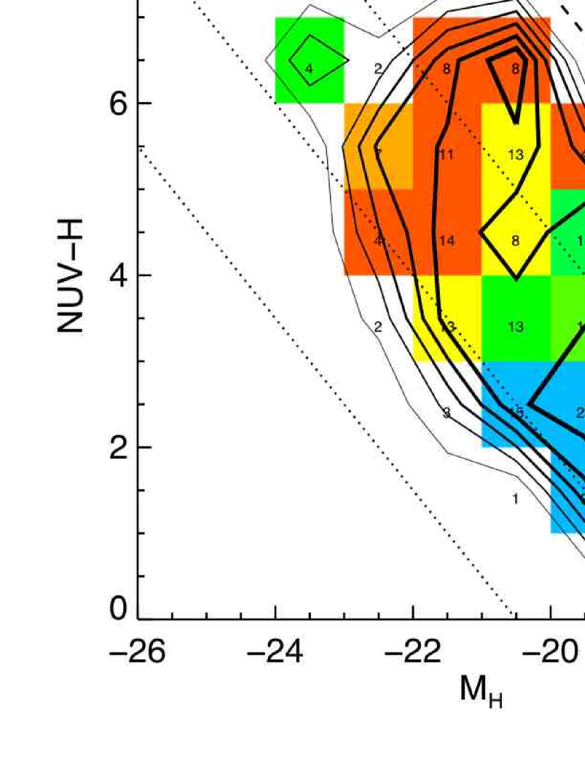
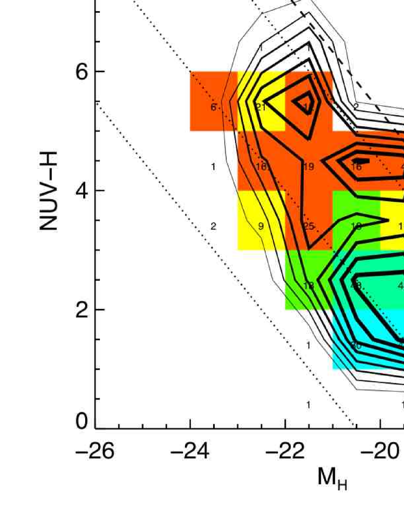
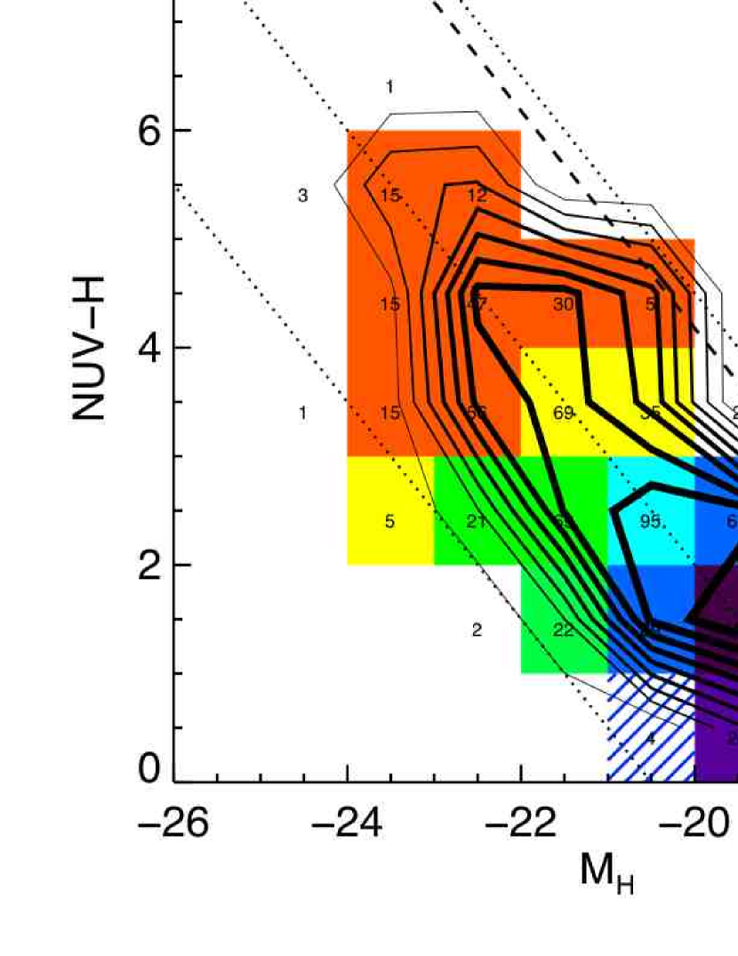
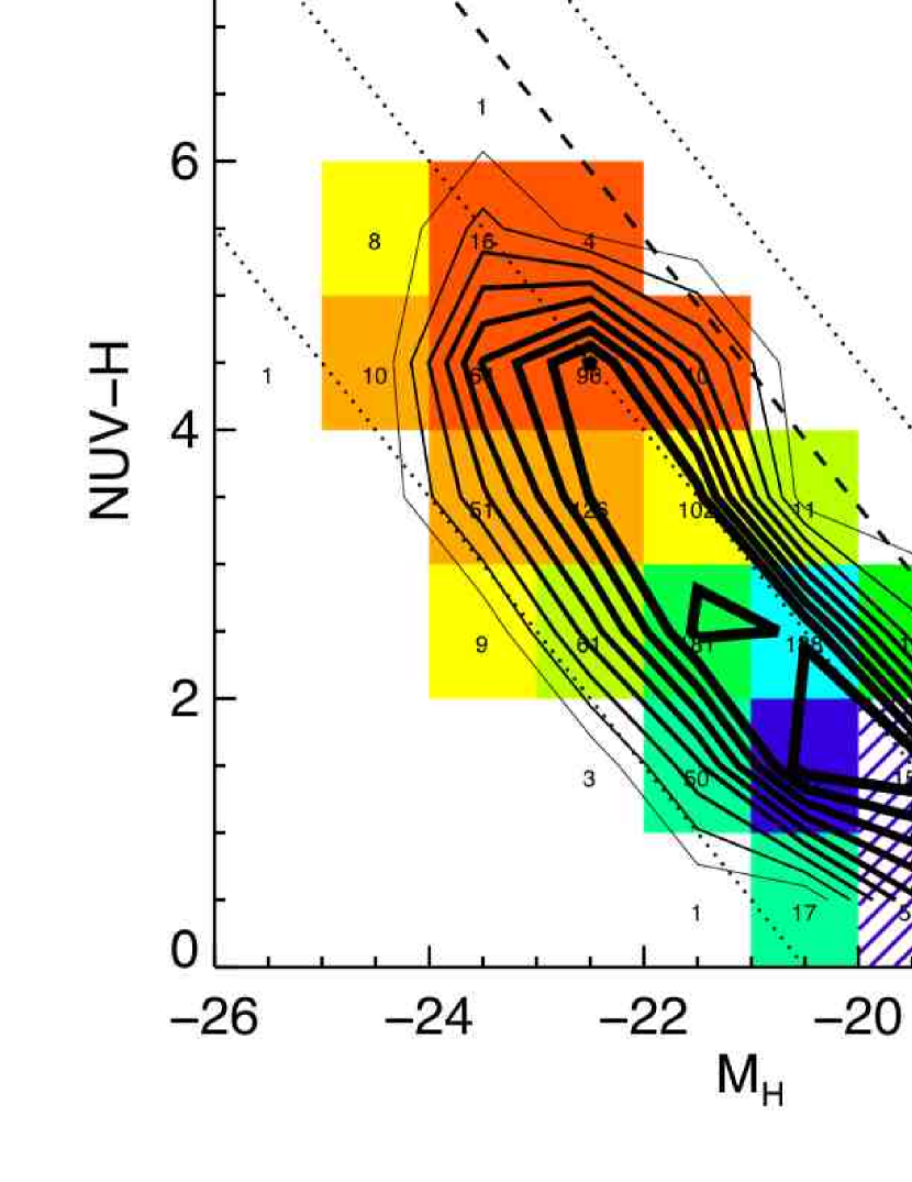
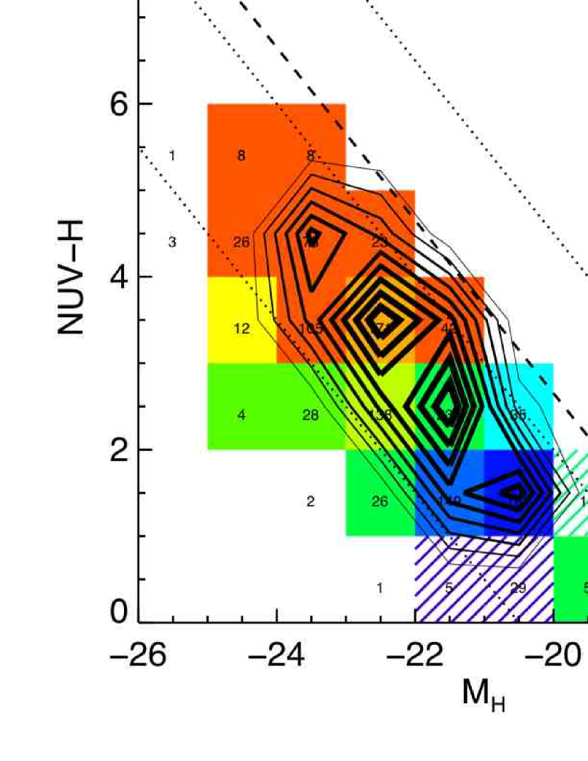
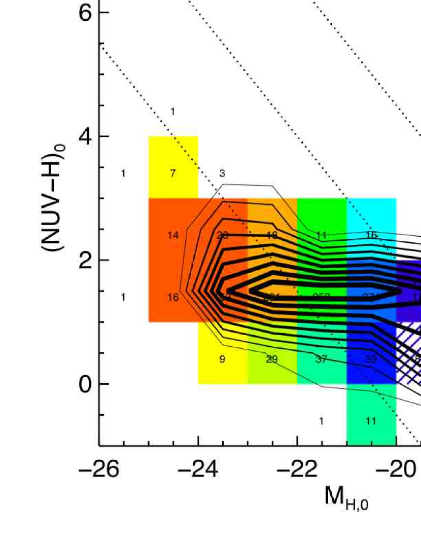
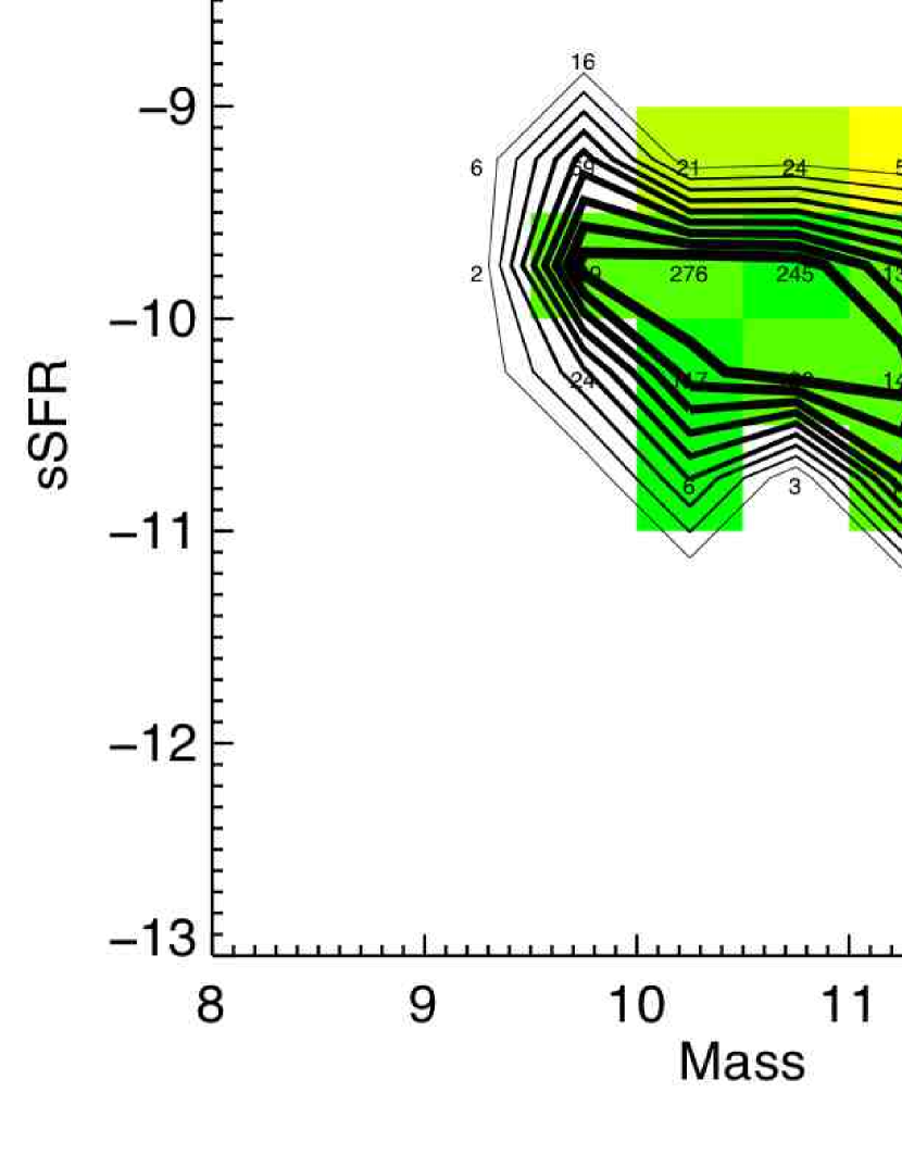
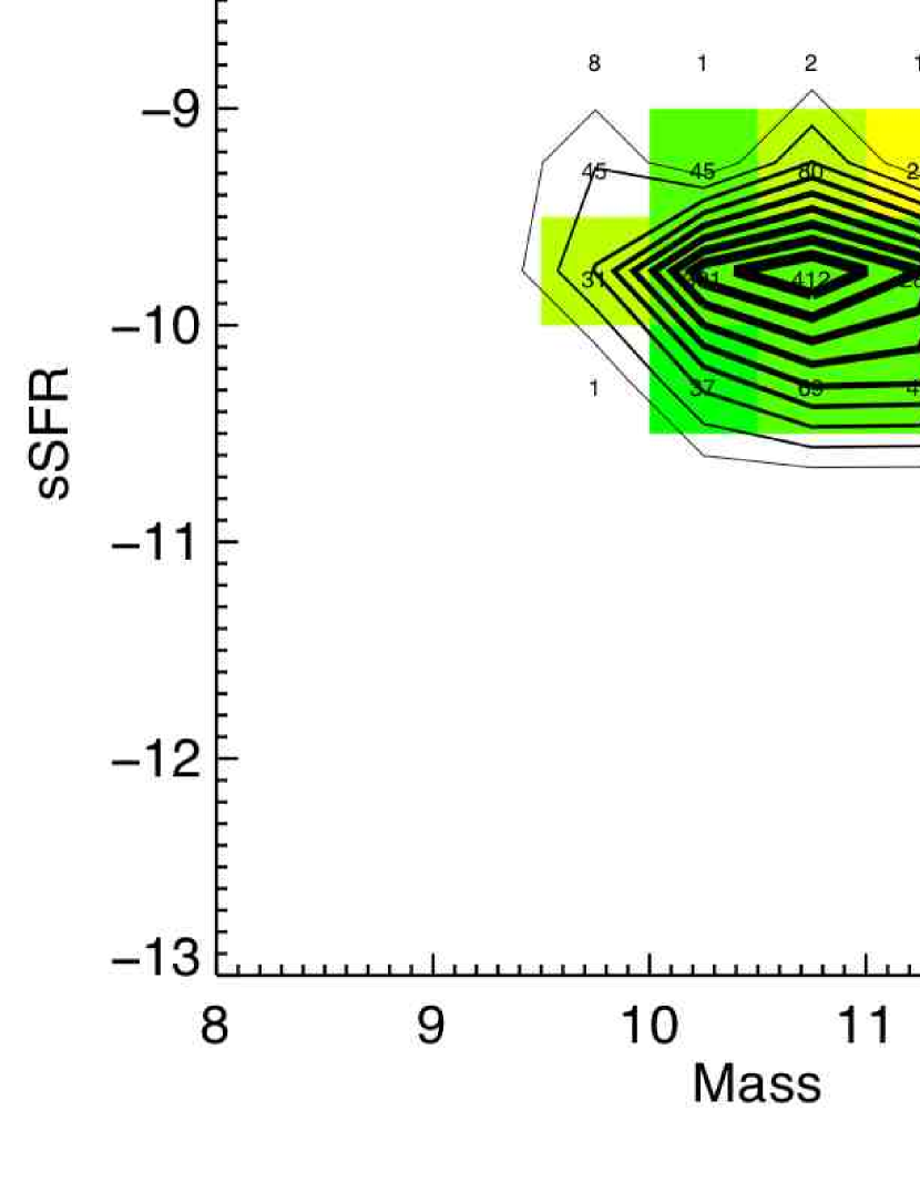
The resulting distribution is displayed in contour plots in Figures 1. The general trend that can be seen is a shift to bluer NUV-H colors and brighter MH magnitudes. These plots also show average IRX in each bin, to be discussed in the next section.
3.3 IR Stacking, Bolometric Correction, Extinction Correction
We have generated an average IRX for each bin in the MH , NUV-H color magnitude diagram. As we discussed earlier, we do this because of the small overlap in UV and MIPS detections. There is considerable evidence that galaxies occupying a single color magnitude bin have a relatively small dispersion in most properties, including extinction (Martin et al., 2007a; Wyder et al., 2006; Johnson et al., 2006a). This approach allows us to estimate the average IRX over a large range of stellar mass and redshift, offering sensitivity to quite low IRX. In order to ensure that the technique is not affected by systematic or random error, we perform a set of tests below.
The basic stacking technique is as follows. We first generate a catalog of detected sources in the MIPS 24 m band using Sextractor. Using this catalog we generate a set of cleaned images with detected sources removed. For each redshift and each color-magnitude bin (NUV-H, MH , z) we stack images in each band that do not have detected sources. We then extract either a source flux or an upper limit, and add this to the detected flux. This results in a flux or upper limit.
We must then make a bolometric correction to the observed 24 m luminosity. We have used the GALEX/SWIRE catalog generated for Johnson et al. (2006a, 2007) to derive the bolometric correction of rest frame flux from 12-24 m (corresponding to 01). We use the measured FIR fluxes and fits to Dale& Helou (2002) SEDs and derive coefficients in the following relationship using log-log fits:
| (3) |
where is the observed rest frame luminosity (). We list in Table 2 the coefficients aλ and bλ. The rms errors in the fits used to derive the coefficients are small, .
Finally, we correct the NUV-H color and H-band magnitude for internal extinction using the IRX and the following prescription based on Calzetti et al. (2000):
| (4) |
where corresponds either to FUV or NUV, and the bolometric corrections are , , and .
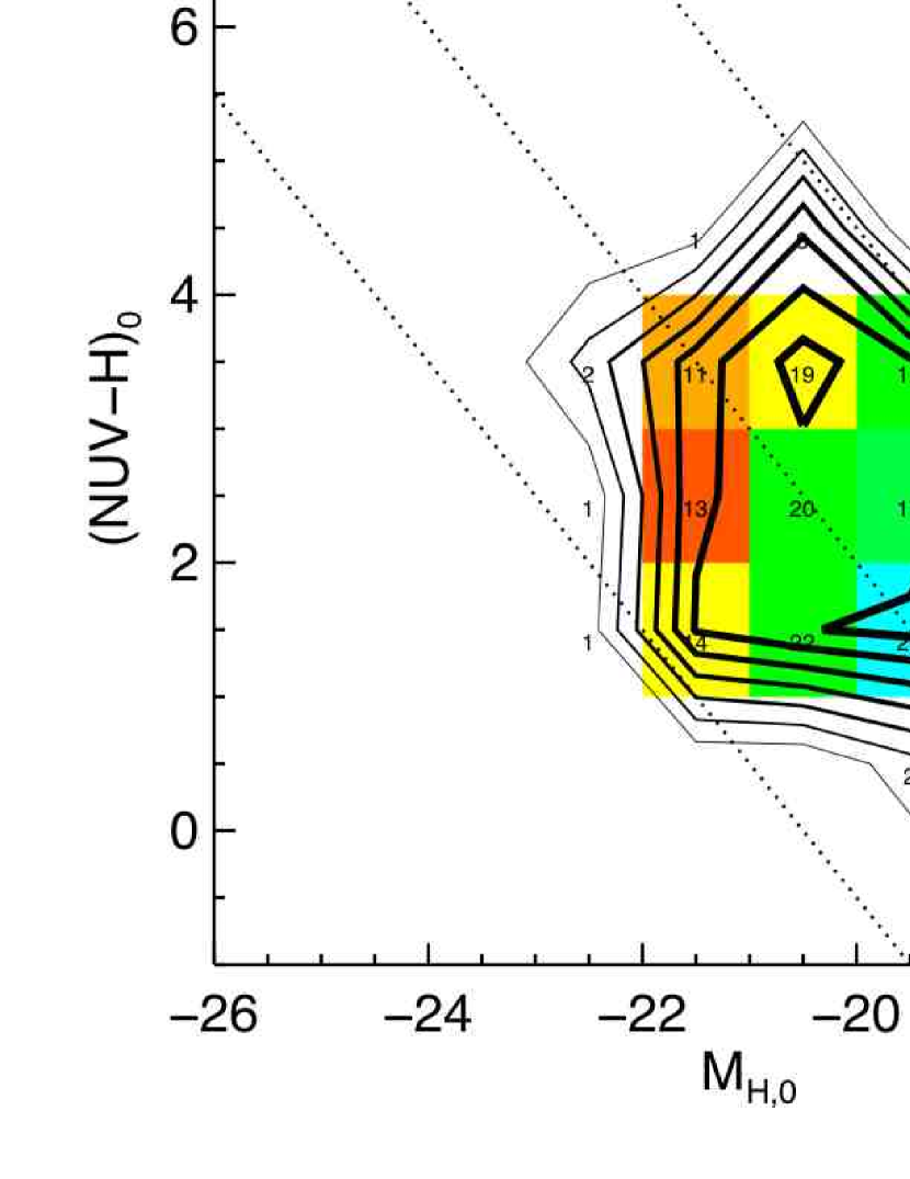
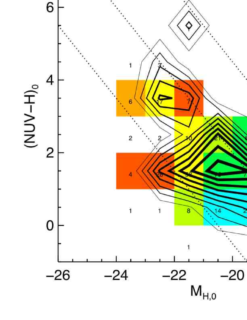
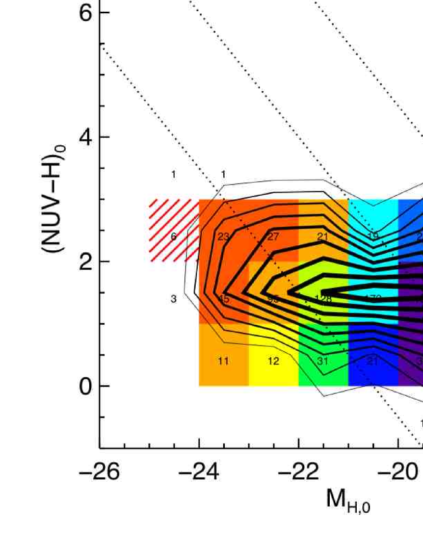
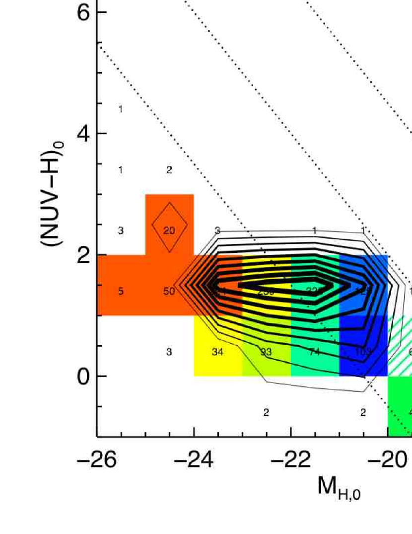
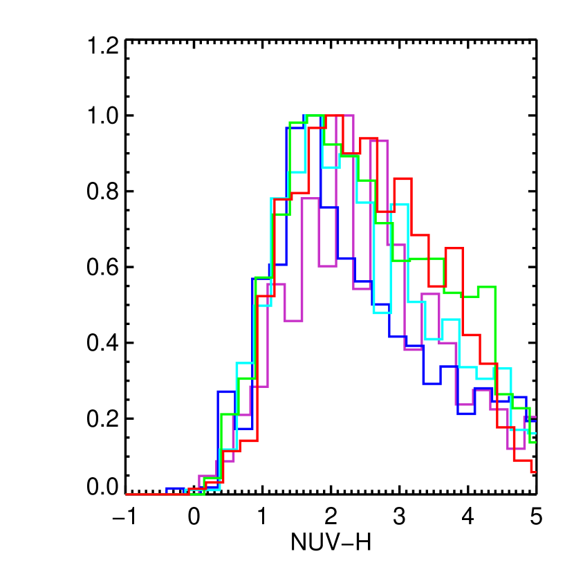
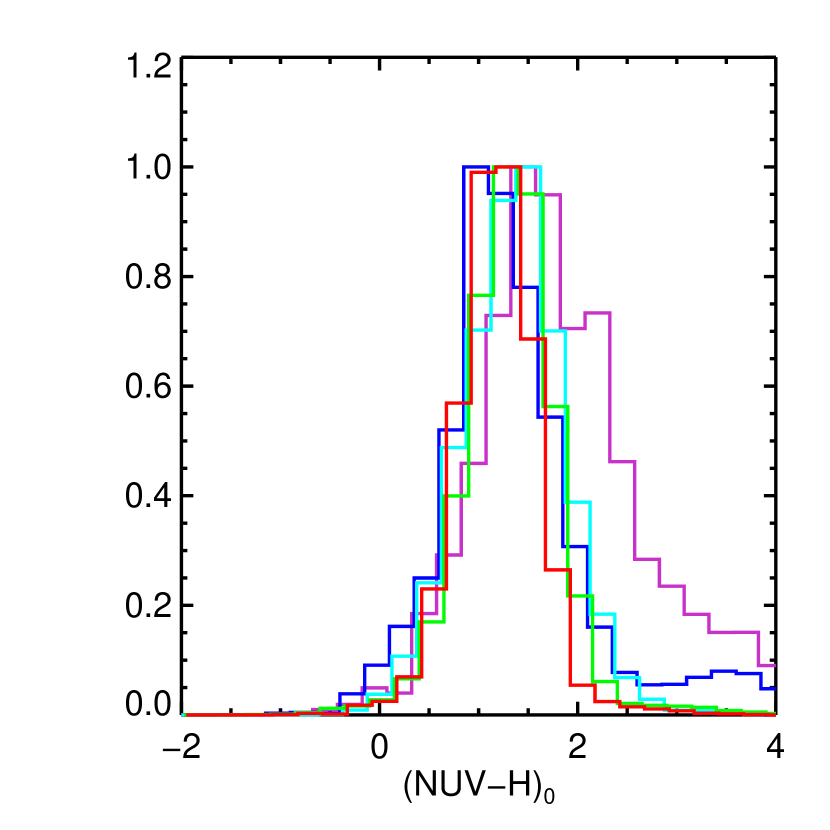
Since the H-band correction is small, the extinction correction is very insensitive to the extinction law. It enters somewhat if we use L(FUV) to generate IRXFUV and use this to correct (NUV-H). Even if there is evolution in the extinction law, we have found that using IRXNUV, gives very similar results to those using IRXFUV. The volume-corrected distribution of extinction-corrected magnitudes (MH 0,[NUV-H]0) vs. redshift are given in Figure 2. We show in Figure 3 the uncorrected and corrected distribution in NUV-H.
3.4 Stellar Mass and Specific Star Formation Rate
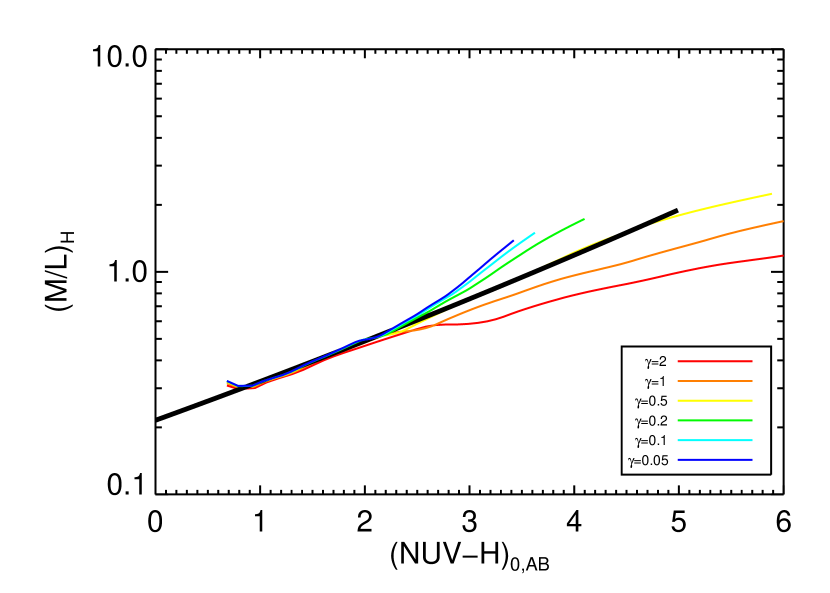
We derive stellar mass using extinction corrected rest-frame H-band absolute magnitude and NUV-H color, following the basic scheme of Bell et al. (2003). For smooth star formation histories the stellar mass-to-light ratio is a single parameter function of a measure of the specific star formation rate such as the rest frame extinction corrected NUV-H color. This can be seen in Figure 4, which shows the predicted vs. (NUV-H)0 for different values of the exponential SFR decay, based on solar metallicity models of Bruzual & Charlot (2003) and a (standard, non-diet) Salpeter initial mass function111Note that all derived stellar masses and star formation rates can be converted to the “Diet Salpeter” IMF of Bell et al. (2003) by multiplying by 0.7 Specific star formation rates are unaffected.. There is almost no dependence on the star formation history for (NUV-H)0 for NUV-H2.5, where the bulk of the extinction-corrected galaxies fall. We use this parabolic fit:
| (5) |
We have also tested more complex star formation histories in which starbursts become significant. These models produce the same general trends between and NUV-H color, with some dispersion. There is no significant impact on the results described below.
We derive the star formation rate from the extinction-corrected FUV luminosity using (Kennicutt, 1998). We obtain the specific star formation rate (SSFR) by dividing by the stellar mass.
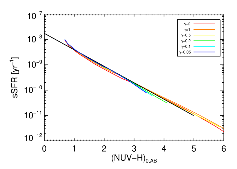
We also note that the specific star formation rate (SSFR) is tightly correlated with (NUV-H)0 and independent of decay timescale, as can be seen in Figure 4. We can also use the following linear fit to convert (NUV-H)0 to SSFR.
| (6) |
Again, either technique for computing the SSFR produces essentially identical results.
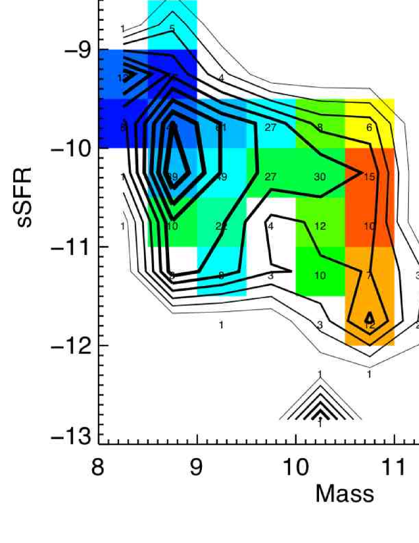
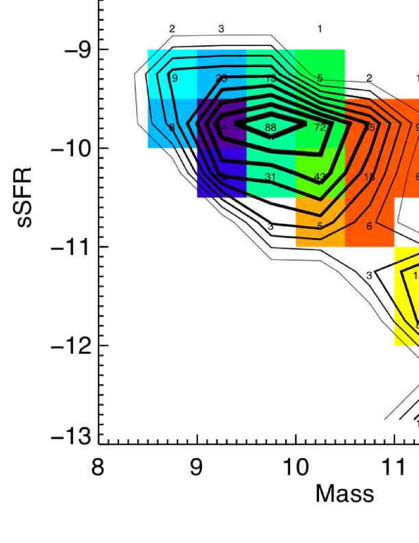
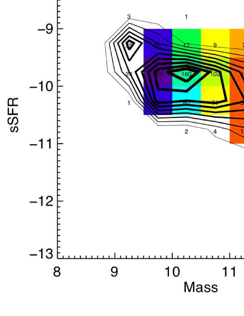
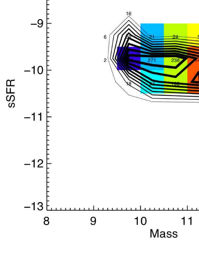
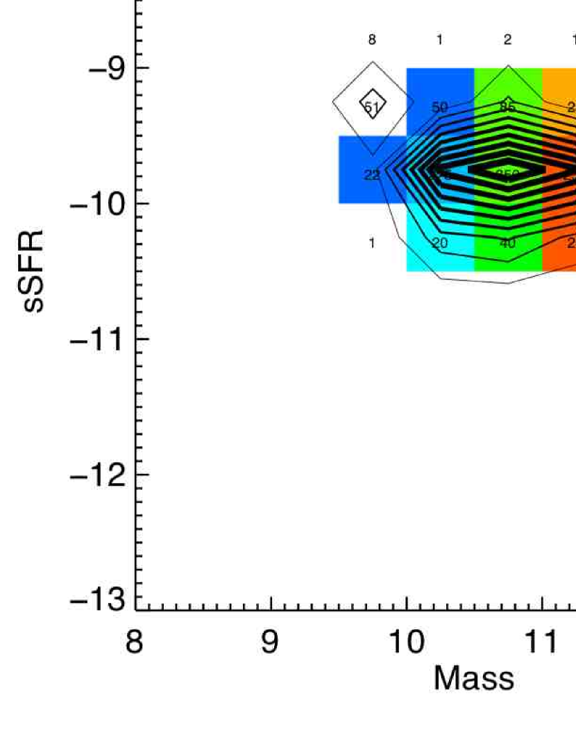
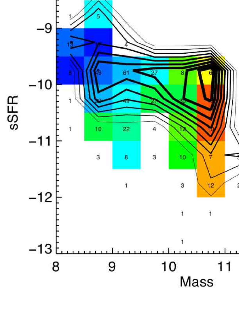
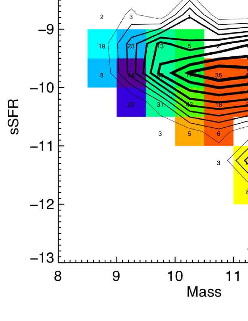
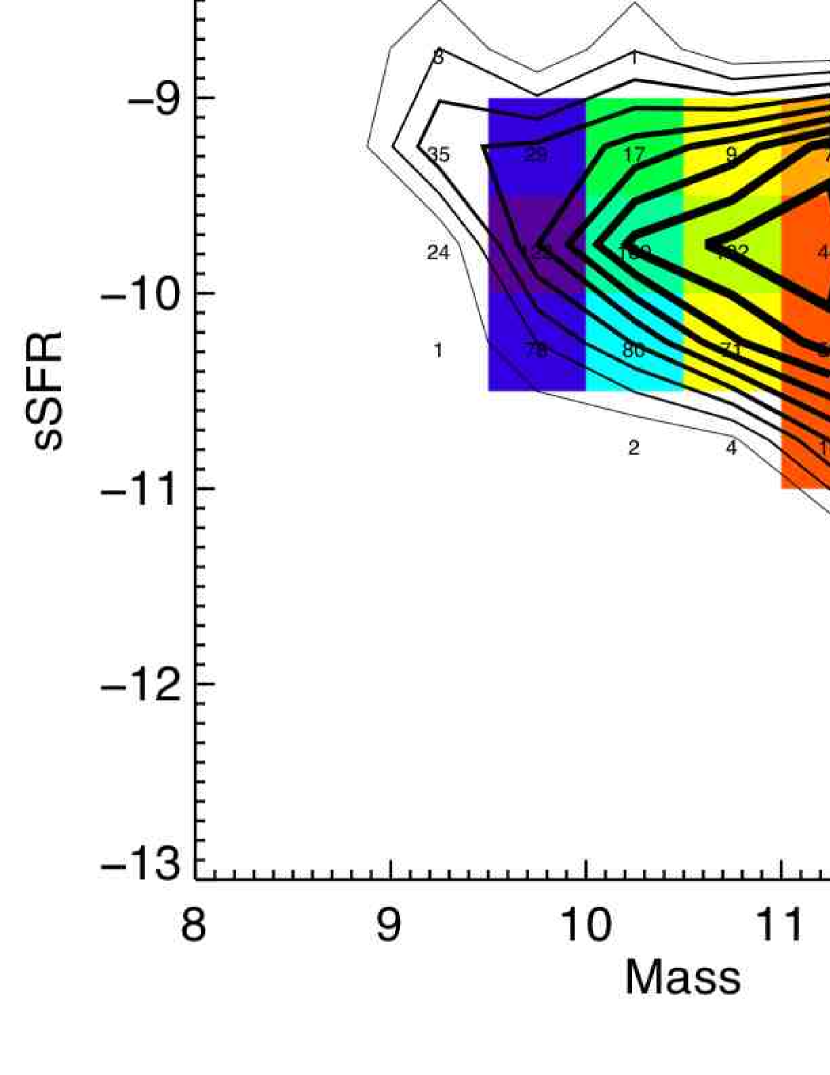
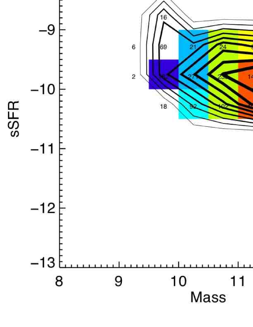
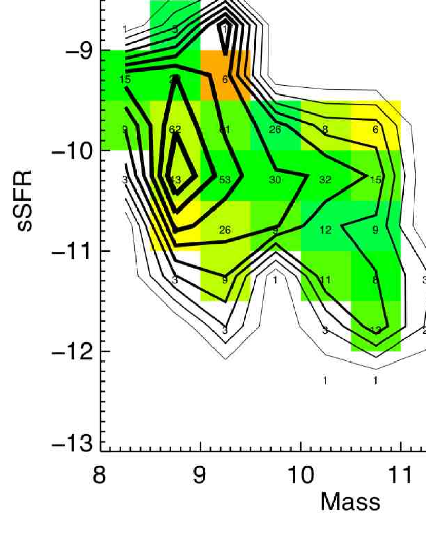
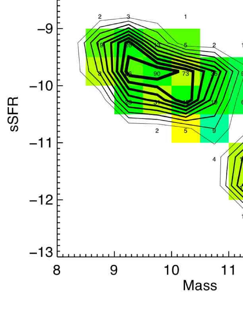
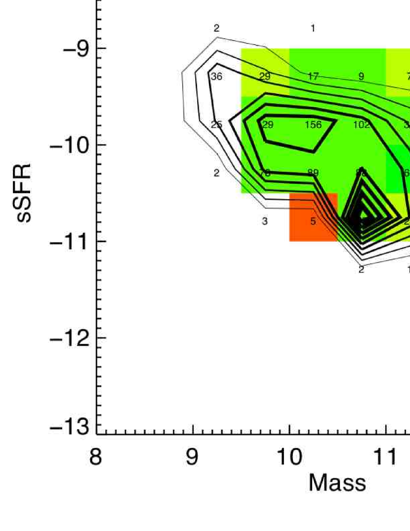
We derive the stellar mass and SSFR for each galaxy by correcting its rest-frame MH , M1500, and NUV-H for the (bin-averaged) extinction. Using these distributions we derive the volume-corrected bivariate -SSFR distribution (,SSFR,z) in the same fashion as the volume-corrected color-magnitude distribution. We also generate an average IRX in each bin of the -SSFR distribution. We calculate the mean log infrared excess in each bin, using the IRX obtained in the previous section. These distributions are displayed in Figure 5.
3.5 Errors
We use the bootstrap method (Efron, 1979) to derive errors to all bivariate distributions discussed above as well as the average distributions discussed in the next section. Specifically, in each redshift bin we randomly select objects, with replacement, until we have the same number of objects found in that redshift bin. We then proceed to determine the color-magnitude distribution, the mean 24 micron flux in each color-magnitude bin by stacking this new sample, the corrected CMD, the Mass-SSFR distribution, and the mean IRX in each Mass-SSFR bin (cf. §4.3). Of order one hundred trials are used to generate a standard deviation in each bin of every distribution calculated. Such errors will not, however, account for cosmic variance due to large scale structure. (cf. §5.2).
4 Results
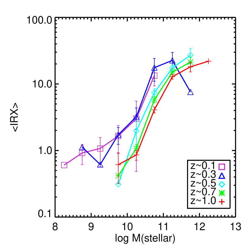
4.1 Infrared Excess vs. Stellar Mass
We begin by examining the trends in the NUV-H, MH CMD. At a fixed MH redder galaxies have a higher IRX. In general, the blue sequence shows a significant tilt in the color-magnitude diagram, much of which appears to be produced by this extinction-luminosity relationship. Much of the color width of the blue sequence, which leads some authors to refer to it as the “blue cloud”, is also produced by variance in extinction (Wyder et al., 2006), some of which is simply due to inclination variations (Martin et al., 2007a). Extinction correction produces a much tighter distribution in the CMD, as we see in Figure 2 and Figure 3. The trend of increasing IRX with H-band luminosity is even more apparent in the extinction-corrected CMD. Consequently, there is a strong increase in IRX with stellar mass as is expected from the trend in the CMD. This trend can be clearly detected in Figure 5. This trend persists in all redshift bins.
4.2 Evolution of the Bivariate CMD
There is clear evolution in the NUV-H, MH color-magnitude diagram, in the sense that the density of H-band luminous galaxies is increasing with redshift. This is consistent with the increase in characteristic UV luminosity (Schiminovich et al., 2005) and B luminosity (Bell et al., 2004). As expected from the previous section, this is accompanied by an increase in the contribution from higher IRX galaxies. The evolutionary trend is even easier to discern in the extinction corrected CMD, Figure 2.
4.3 Infrared Excess vs. Stellar Mass and Redshift
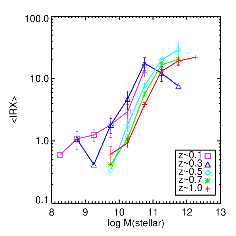
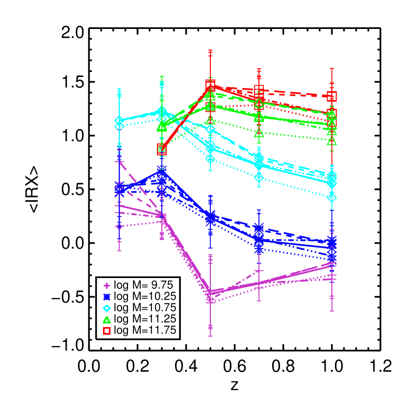
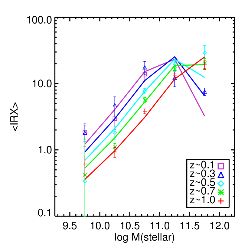
In order to further explore IRX-mass relationship and its evolution we derive the average IRX in each mass and redshift bin. We have calculated this average using the number density () and weighted by the star formation rate SFR(). The mass trend in redshift bins is shown in Figure 7. The average IRX increases sharply with mass up to a critical mass. The slope in the in the IRX-log mass relation is greater than one. The critical mass is lower at low redshift, at z0.3, but appears to move to higher mass at higher redshift, with at z1.
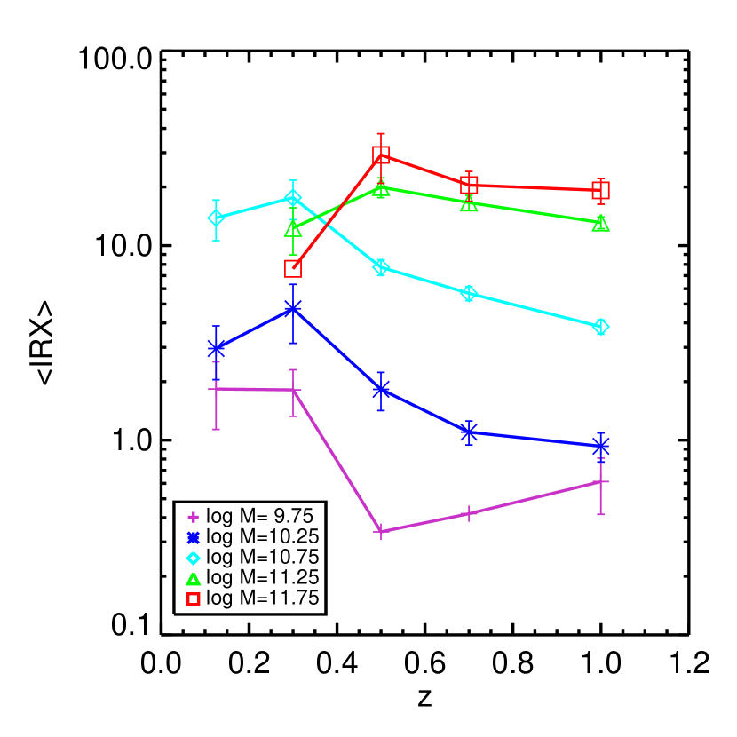
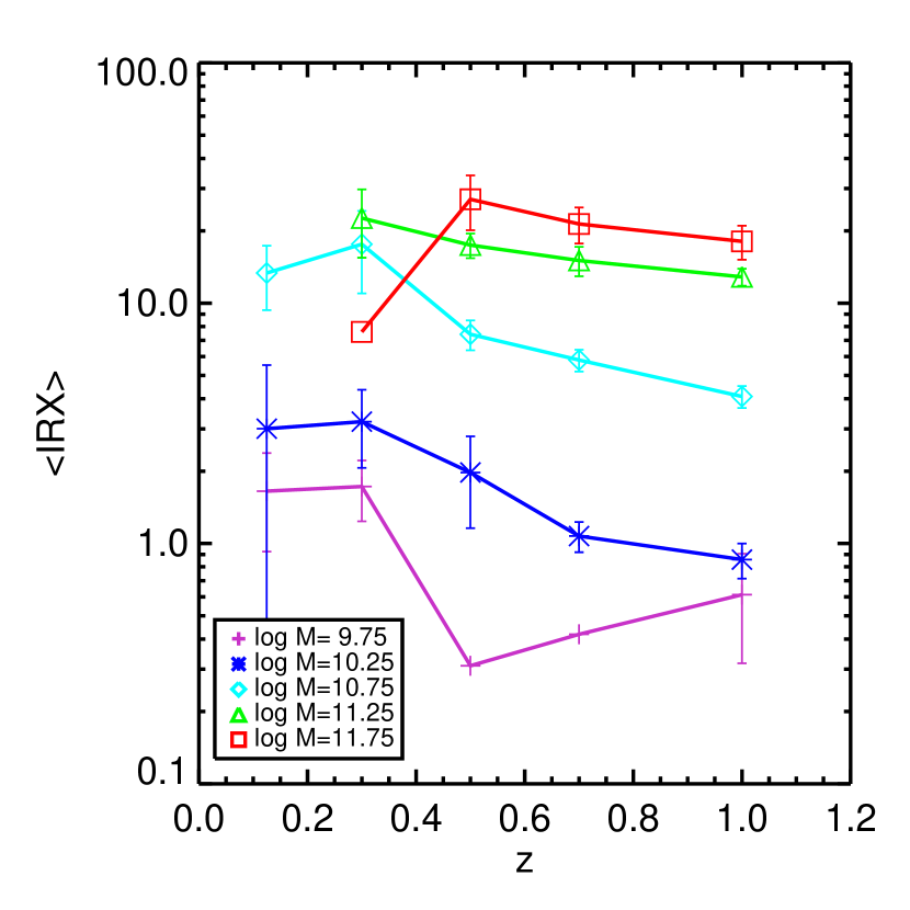
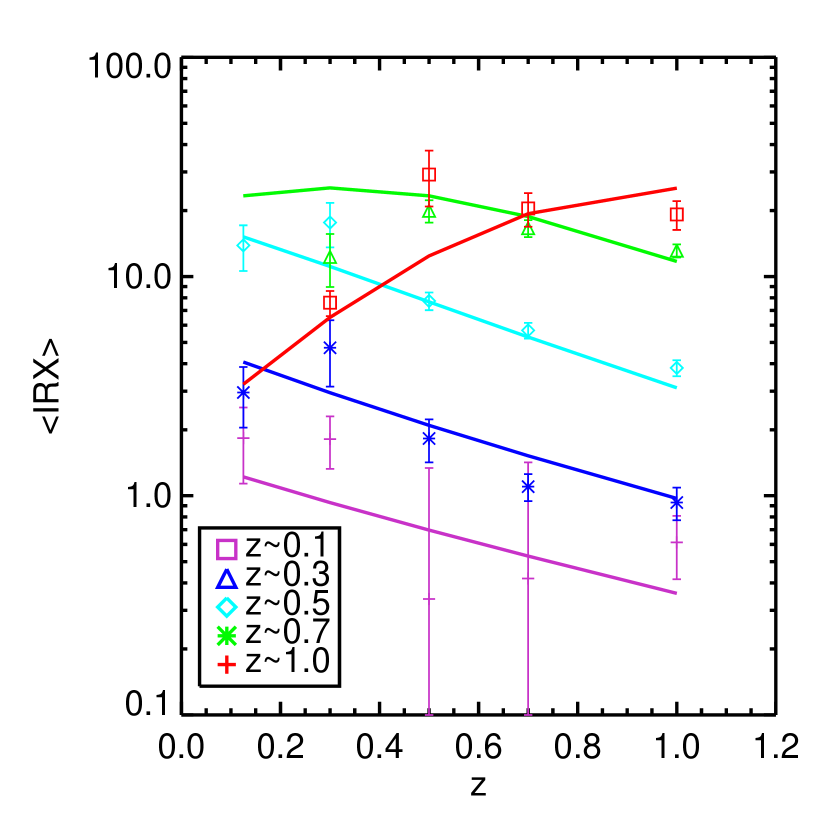
The redshift trend in mass bins is shown in Figure 8. In the highest mass bin with good redshift coverage (), IRX increases slowly with time then sharply decreases for z0.5. In the lowest mass bin, IRX appears to increase with time to the lowest redshift bin. These trends appear in both the number and SFR-weighted average IRX. For our subsequent analysis we use the number-weighted average.
4.4 Co-evolution of SFR and IRX
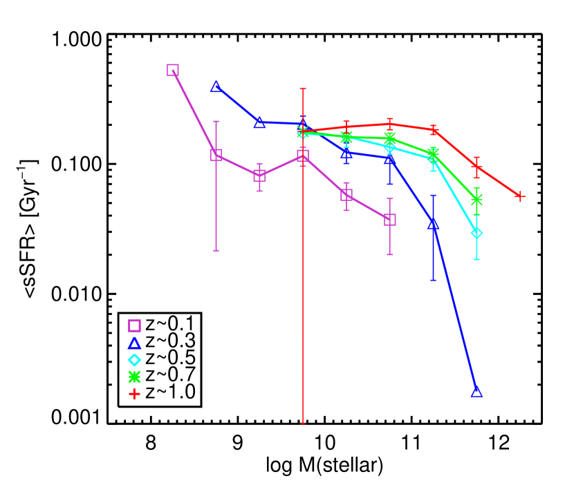
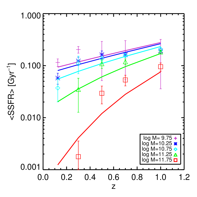
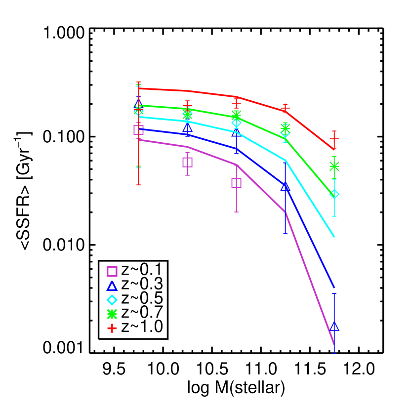
We have seen that the star formation rate density is moving to higher masses at higher redshift. This can best be seen in the SFR-weighted bivariate -SSFR distributions shown in Figure 6. It is interesting to determine the average SSFR vs. mass and redshift as we did for IRX. The number-averaged SSFR is given in Figure 9. This shows that at lower mass, , evolves slowly, while at higher masses the SSFR falls rapidly with time.
The behavior in Figures 7-9 can be explained by a simple model. We suppose that average IRX is determined principally by the gas surface density and by the metallicity. This naturally produces a rising then falling IRX as the gas becomes enriched (in a closed box model) and then exhausted. Downsizing implies that star formation, enrichment, and ultimate gas exhaustion move to lower masses with time, consistent with these resullts.
We examine this model further in the next section. But first we ask whether the observed trends could be an artifact of selection effects or other aspects of our technique.
4.5 Issues and Caveats
We have performed a number of tests to ensure that the results presented above are not a product of the samples or analysis approach.
We could use either FUV (1530Å) or NUV (2270Å) flux to derive star formation rates. Since we bin and stack sources in the NUV-H CMD, there could be systematic effects introduced by either the use of an extinction law to correct FUV given the NUV-derived IRX, or there could be effects introduced by the different data samples used to derive FUV and NUV rest luminosities. The former come completely from GALEX data, while the later come from interpolating GALEX and COMBO-17 data. We find however that there is no significant difference in the results using FUV or NUV to derive IRX and SFR.
We tested stacking the MIPS24 data using detected sources and cleaned images, and using only the fluxed images (stacking detected and undetected sources together). This produced no statistically significant difference. We also were concerned about the MIPS24 detection limit and whether the low limit of 0.02 mJy used to detect and clean the images would include some spuriously detected sources due to confusion, yielding an artificially high 24 micron flux in the stacked result. We checked this by increasing the detection limit by a factor of two and repeating the entire analysis. Again, these results showed only minor quantitative changes.
A very important question is whether our census of objects is complete. We could be missing FIR luminous objects that fall below the UV magnitude limits of the sample. Moreover, it is likely that as we move to higher redshift, more of the high IRX and/or low SSFR sources are lost due to the UV magnitude limit. This could clearly introduce a spurious blueing trend as redshift increases, which is exactly what we detect.
To test for this effect, we repeated the analysis on the following samples: 1. Baseline: NUV26.0, r24.0; 2. Case 2: NUV25.0, r24.0; 3. Case 3: NUV27.0, r24.0; 4. Case 4: NUV26.0, r25.0; 5. Case 5: all r24.0 objects, whether or not detected in NUV. Those objects below the NUV detection limit are given an artificial magnitude NUV=27.0. The average IRX vs. redshift for these cases is shown in Figure 10. There are no significant changes to or in the observed trends with mass and redshift.
Another test is to consider the inclination bias of the sample. A sample at high redshift which has not included highly inclined, more reddened galaxies of otherwise similar overall dust content will display a higher average minor to major axis ratio than the low redshift counterpart. The average axis ratio obtained from the (seeing limited) COMBO-17 data shows no significant trends with redshift. This is true in the MH , NUV-H CMD and as we show in Figure 11, the final -SSFR diagram.
Finally, we used a Monte Carlo model to test whether the evolving IRX-mass relationship could be an artifact of the sample selection. The model is semiempirical and we briefly summarize it here. The model predicts the bivariate luminosity function in the extincted, rest-frame NUV-H, MH CMD, and the distribution of over the same CMD ([MH , NUV-H]). The number distribution is given by a Schechter function in mass. The SSFR is log-normal with a constant mean and variance to a certain critical mass, then falls. IRX is log-normal and the mean IRX scales with mass. Evolution is introduced into the number density, mean SSFR, SFR cutoff mass, and the IRX-mass relationship. In the latter case, the following relationship is introduced:
| (7) |
where is a normally-distributed random variable. This assumption allows for IRX dependence on mass, and evolution of this dependence in a mass-dependent fashion, in other words the evolutionary trends we appear to detect in the data.
We convert mass, SSFR, and IRX into observed SED’s using (in reverse) the identical transformations that we used for the data. SEDs are redshifted and run through detection filters with appropriate completeness functions. We then subject the list of objects and observed FUV, NUV, R-band, IRAC, and MIPS24 fluxes to the identical analysis steps as the actual sources, producing the various distributions. (We do not simulate the actual image formation and detection process). Finally, we compare the Monte Carlo and data distributions using a chi-square statistic. For this comparison we combine data and Monte Carlo errors (data errors calculated from bootstrap, Monte Carlo errors calculated from Poisson statistics). To calculate we use all bins in which either data or Monte Carlo results are predicted. We simultaneously fit both and over all five redshift bins.
Because the model has parameters, it is difficult to guarantee any given local minimum is the global minimum. Extensive experimentation has shown that the distribution and IRX distributions are mainly influenced by separate variables, so some minimization can be decoupled. We find best fits with 1.5 and , with and with small formal errors (). The latter are derived in the usual way by fixing the parameter of interest and marginalizing over all others. The key conclusion is that the significant non-zero value of provides additional evidence that the evolving IRX-mass relationship is not an artifact of the sample selection.
5 Discussion
5.1 Simple Extinction, Metallicity, and Star Formation Evolution
The phenomena displayed in Figures 8 and 7 have a very simple interpretation. At low mass, ongoing enrichment by star formation increases the dust-to-gas ratio and mean extinction per unit gas, resulting in a steady growth in IRX. Higher mass galaxies had their periods of peak star formation in the past, and the exhaustion of their star forming gas supply (by whatever mechanism) leads to an IRX which falls with time. We reiterate that our determination of IRX is obtained directly from the Far UV-to-Far IR ratio (the latter from 12-24 m luminosity and a bolometric correction), and is independent of the extinction law.
We can model this using the classical exponential SFR models introduced by Tinsley (1968) and a very simple extinction model. The SFR obeys:
| (8) |
where is a scale-free “age” parameter.
For simplicity, we characterize the extinction as if it occurs in a simple foreground absorbing slab of dust, and that its strength tracks the amount of gas responsible for star formation:
| (9) |
where is the metallicity (we assume that gas-to-dust ratio scales accordingly), and is the gas surface density. Ignoring inclination induced anisotropies, we have . Let us further assume a Schmidt-Kennicutt scaling law (Kennicutt, 1989) . Here we note . Then
| (10) |
In a closed-box enrichment model, metallicity grows as
| (11) |
for an exponentially decaying SFR. The gas fraction is and is the average yield (Searle & Sargent, 1972). Thus we expect
| (12) |
Here is a scaling constant appropriate for an average inclination.
This can be generalized to the leaky-box case (Hartwick, 1976) in which the outflow is proportional to the star formation rate . In this case
| (13) |
If then an accreting-box case (Binney & Merrifield, 1998) with infall proportional to SFR would obtain. We do not consider other accreting-box scenarios.
Finally, we need to relate the age parameter to galaxy mass. 222We label galaxies by their stellar mass. Over the redshift range we consider, a constant SFR would increase the stellar mass by 0.5 dex, or one mass bin. We ignore this subtlety in order to make the arithmetic simple for this very basic model. We make a simple ansatz that the age scales as mass to a constant power , that a single formation time is appropriate, and that the past age is reduced by the relative elapsed time from formation:
| (14) |
The specific star formation rate (SSFR) is given for this model very simply by:
| (15) |
where is a function of mass for a coeval population: .
We jointly fit the and vs. mass and redshift with five free parameters: , , , , and . We restrict the fits to the mass range , over which the survey appears reasonably complete at all redshifts (cf. below). There are 46 independent data points and four free parameters. The result is a reasonable fit, with , with , Gyr, , , and . Note that for Schmidt-Kennicutt star formation law we expected . The fits are displayed in Figure 12 and 13. Using this we predict that the mass metallicity relation shifts towards higher masses roughly at and at , not inconsistent with Savaglio et al. (2005). This also predicts a peak equivalent extinction at of , or peak=1.2. The only way to distinguish between the closed and open box cases is to provide an independent measurement or prediction of the proportionality constant , which is beyond the scope of this paper.
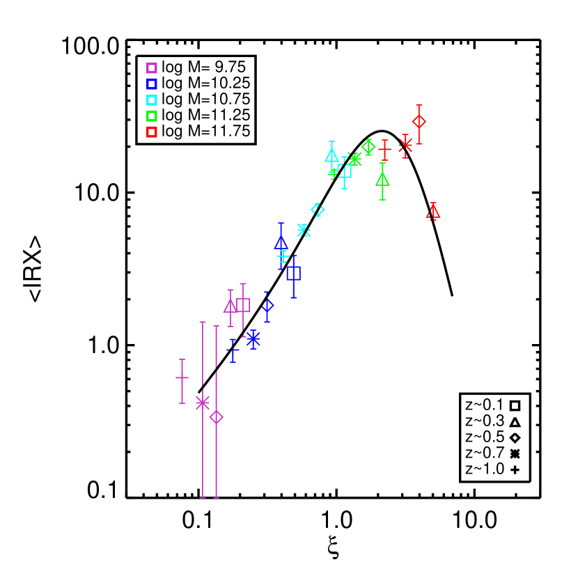
We show the tight relationship between the age parameter , derived from the stellar mass and the best fit parameters:
| (16) |
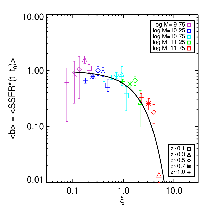
and the mean IRX at in Figure 14. There is an equally tight relationship between the “b-parameter” which in terms of our simple parameterization is:
| (17) |
This is displayed in Figure 15. Finally, we show the co-evolution of and in Figure 16.
We can also define a “turnoff” mass where so that
| (18) |
which rises from at z=0 to at z=1. We note that is exactly the transition mass between star forming and passively evolving galaxies noted by Kauffmann et al. (2003) in the SDSS spectroscopic sample.
Metallicity and age are simply related in this picture (cf. equation 11). Johnson et al. (2007) have shown that IRX correlates well with metallicity. The mass-metallicity relationship (Tremonti et al., 2004) is a result of the lower net astration in galaxies with a younger effective age . This simple picture does not predict the observed saturation at high mass. This could be a result of selection effects, since metallicity can only be measured using emission lines in galaxies with high SSFR. It is plausible that transition galaxies with low emission line equivalent widths display a higher metallicity than the actively star forming sample at high mass. It could also indicate a second quenching mechanism in addition to simple gas exhaustion, or a more complex enrichment picture than simple closed box evolution.
5.2 Star Formation History and Evolution of the Blue and Red Sequence
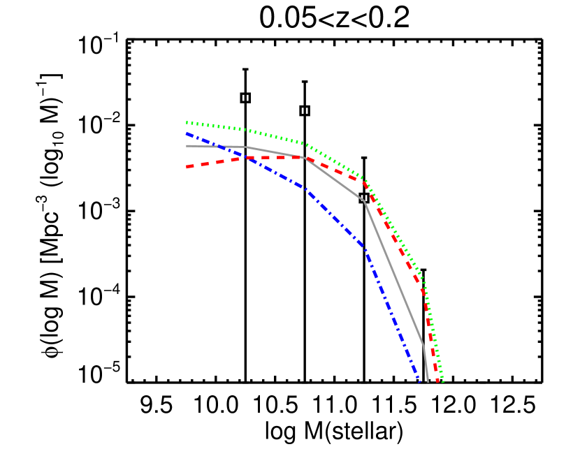
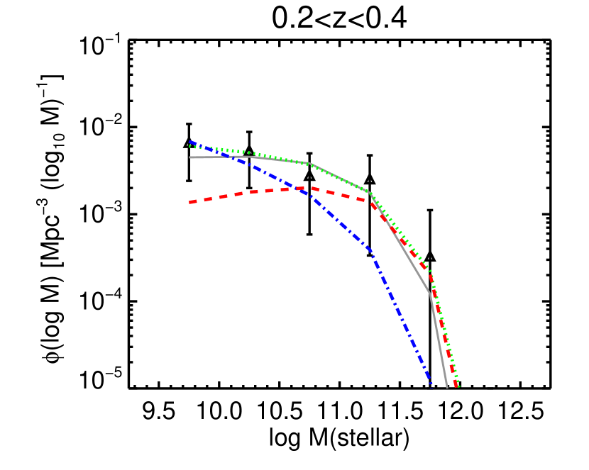
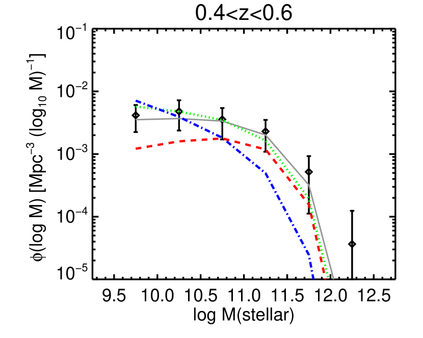
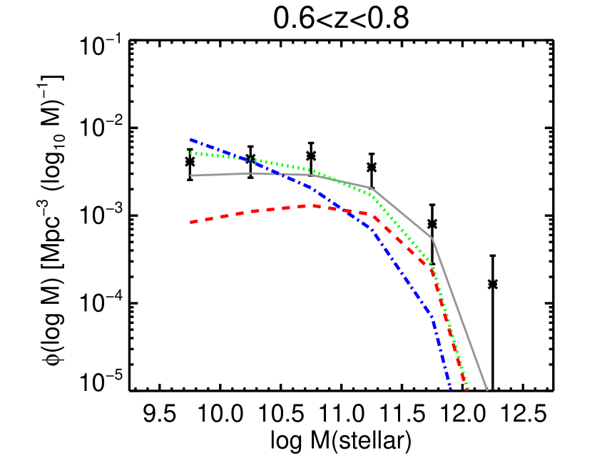
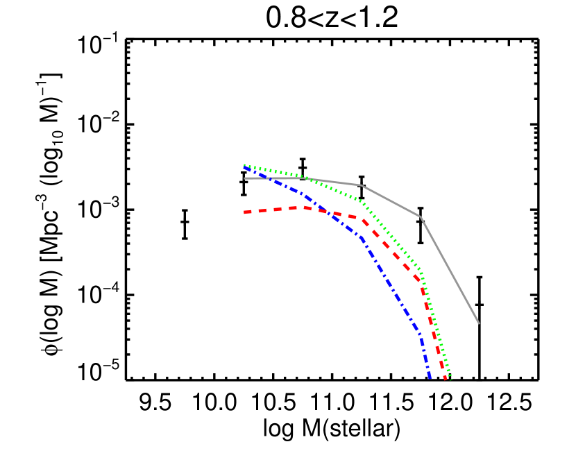
We begin by determining the mass function by summing over SSFR in the bivariate mass-SSFR function. The distribution in each redshift bin is displayed in Figure 17. The error bars include Poisson and cosmic variance, the latter from Somerville et al. (2004). Note that these combined errors will be highly correlated between mass bins at a given redshift. This correlation is not well represented by the plotted error bars, since there is large covariance between mass bins in a given redshift bin. Note also that there is evidence for incompleteness in the lowest mass bin () for z=1.0. Mass bins were not used in the modelling of the previous section, because of obvious incompleteness.
We model the mass function as an evolving Schechter function:
| (19) |
where and . We use a version of chi-square minimization that accounts for the cosmic variance and covariance between mass bins in a single redshift bin (e.g., Newman & Davis (2002)) The best fit parameters and one sigma errors (obtained by marginalizing over other parameters) are
| (20) | |||||
| (21) | |||||
| (22) | |||||
| (23) | |||||
| (24) |
The non-zero values of and indicate evolution in the characteristic mass and the number density, although cosmic variance prevents tight constraints on the evolutionary indices. Note we have not parameterized an evolving low mass slope.
We can compare the results of this mass function analysis with the results of Bell et al. (2003) using a much larger cosmic volume at . Converted to our cosmology and corrected upward to a non-diet Salpeter IMF (simply dividing their result by 0.7), they obtain Mpc-3 , and for all (late-type) galaxies vs. our values at z=0.125 Mpc-3 , and . The mass cutoff is in fair agreement, but our density is a factor of 2 larger if we compare to just their late-type (morphologically selected) sample. The mass cutoff, slope and density parameters are highly correlated, and indeed if we fix our mass cutoff (z=0) at 11.1 (which is within our errors) we find Mpc-3 , close to the Bell et al. (2003) value. If we fix the slope to we find Mpc-3 and . Thus our results at are consistent with Bell et al. (2003) within the errors quoted above (dominated by cosmic variance).
We can also compare to the evolving Borch et al. (2006) mass function which uses all three COMBO-17 fields with a total of 25,000 galaxies. We correct their masses to our standard Salpeter IMF by multiplying by 1.8, as they suggest. At z=0.9, they obtain Mpc-3 and , again for all (blue, color-selected) galaxies. Using our evolutionary parameters, we find Mpc-3 and . Our results are compared to Borch et al. (2006) in Figure 17. Surprisingly, our results agree well with theirs for the entire galaxy sample in all but the highest redshift bin. Our bin extends over (0.8¡z¡1.2), while theirs is (0.8¡z¡1.0). Our mass function shows a distinctly higher mass cutoff in the two highest redshift bins, which leads to the stronger evolution in the characteristic mass.
Searching for an explanation of this difference, we note that a significant fraction of our sample has red colors. In the lowest redshift bin this is true even after the extinction correction. For example, if we eliminate galaxies with , corresponding to corrected , which from Figure 3 can be seen to exclude the tail of the distribution, the mass function density parameter at z=0 falls by a factor of two. This suggests that a significant fraction of the mass (and even the star formation rate) at low redshift is locked in high mass galaxies with low specific star formation rates and red intrinsic (unextincted) colors. Some of these galaxies could be classified as early-type in Bell et al. (2003) because their observed colors are even redder (as they are massive and exhibit high IRX) while their morphologies could be dominated by an evolved, bulge-like component. The steepness of the slope parameter obtained for color-selected blue samples (Bell et al., 2003) could also be a reflection of excluding extincted, reddened higher mass galaxies and transition galaxies that still show some star formation.
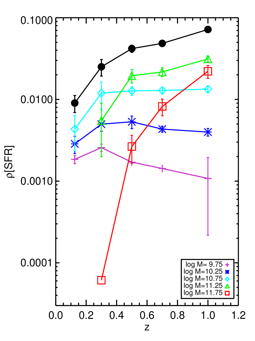
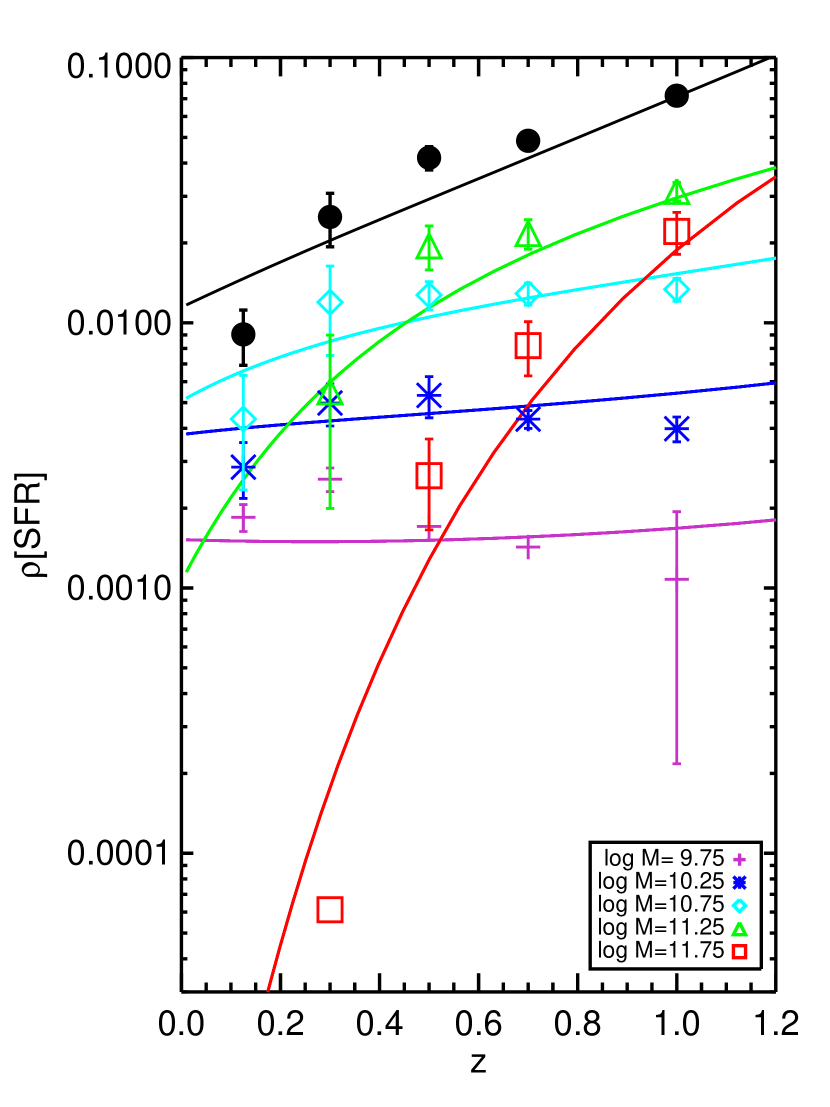
The characteristic mass increases with redshift, with , which can be compared to the model change of from 10.5 to 11.24. Thus the blue sequence mass function shows directly the effects of downsizing. The total mass of the blue sequence obtained by integrating the mass function is a declining function of redshift (since ), M⊙ Mpc-3 (from z=0.8 to z=0). Others (Borch et al., 2006; Blanton, 2006) have found that the blue-sequence mass is constant with time, and giving the uncertainty our results are not inconsistent with this conclusion. In our model this occurs because the mass of the blue sequence is moving from fewer massive galaxies to larger numbers of lower mass galaxies. The decrease in blue luminosity density (e.g., Bell et al. (2004); Faber et al. (2005)) is a result of an increase in mass-to-light ratio due in turn to the falloff of the specific star formation rate. The total stellar mass appears to remain constant or decline in spite of the formation of new stars. Before exploring this point, we estimate the star formation rate density and its evolution.
In order to calculate the star formation rate history while minimizing the effects of cosmic variance, we renormalize the observed mass function to the fit given in Figure 17 and Equation 20 for all redshift bins. The results in each mass bin and the total are shown in Figure 18. We also calculate the star formation rate density evolution for the simple exponential model of the previous section. This is shown in the right-hand panel of Figure 18. Apparently the dominant galaxy population responsible for the fall in SFR density from z=1 to z=0 is (cyan and green points). This is consistent with the conclusion that the characteristic mass derived in the previous section evolves from to . Zheng et al. (2007), also using COMBO-17 and Spitzer data, and the stacking technique of Zheng et al. (2006), have reached conclusions that in many ways are similar to ours, but differ in some important details. In particular, they find that the SFR in the highest mass bin (log M11.25 when converted to our IMF) does not fall more steeply than that in the lower mass bins.
Stars formed over will increase the total mass of the blue sequence unless these galaxies transition to the red sequence. In order to maintain the constant or declining blue-sequence mass, we calculate that the average mass flux over must be ⊙ yr-1 Mpc-3. This is in agreement with the value we obtained by examining transition galaxies at (Martin et al., 2007a).
6 Summary
We have used COMBO-17, Spitzer, and GALEX data to study the co-evolution of the IRX and star formation for galaxies over the mass range of and the redshift range . We have reached a number of interesting conclusions:
-
1.
IRX grows with stellar mass in a way that mirrors the mass-metallicity relationship. The rise of IRX with mass saturates at a characteristic mass, above which it appears to fall.
-
2.
The SSFR is is roughly constant up to the same characteristic mass, above which it falls steeply.
-
3.
The characteristic mass grows with redshift.
-
4.
At a given mass below the characteristic mass, the IRX grows with redshift.
-
5.
The mass and evolutionary trends of the IRX and SSFR are reasonably fit by a simple gas-exhaustion model in which IRX is determined by gas surface density and metallicity, metallicity grows with time following a closed box model, and SFR is determined by the exponentially falling gas density. The SFR time constant scales with the mass as .
-
6.
The characteristic mass is a “turnoff” mass indicating galaxies that are starting to move off the blue sequence.
-
7.
The mass-metallicity relationship is understood to be determined largely by he characteristic age of the galaxies. The mass-IRX relationship is also influenced by gas exhaustion above the turnoff mass.
-
8.
The factor of 6-8 rise in SFR density to z=1 is predominantly due to galaxies in the mass range , the turnoff mass over the redshift range.
These observations show directly the steady build-up of heavy elements in the interstellar media of evolving galaxies, and that the infrared excess IRX represents an excellent tool for selecting similar mass galaxies at various stages of evolution. In particular, galaxies at early stages in their evolution can be selected by their low IRX (Figure 14).
It is important to stress that these trends were uncovered by considering the average properties, notably the IRX, of large numbers of galaxies. A more sophisticated treatment would study the detailed distribution of properties, for example the spread in SSFR in a given mass bin. The simple scaling model of course predicts no spread at all for a coeval population. This distribution may yield information about the burst and formation history of galaxies. For example it will be very interesting to study galaxies with an unusually low IRX at a given epoch and mass to determine whether they are more recently formed. It will also be interesting to compare this very simple picture with the results of semianalytic models combined with the latest numerical simulations. Finally, it is critical to improve the observational basis of this work, most notably with a better understanding of the FIR bolometric correction and its evolution, with a larger and deeper sample of galaxies, and by extending the redshift range of this approach to determine whether this simple picture continues to apply during the major epoch of star formation.
References
- Adelberger & Steidel (2000) Adelberger, K. L., & Steidel, C. C. 2000, ApJ, 544, 218
- Bell et al. (2003) Bell, E.F., McIntosh, D.H., Katz, N., & Weinberg, M.D. 2003, ApJS, 149, 289.
- Bell et al. (2004) Bell, E. F., et al. 2004, ApJ, 609, 752.
- Bell et al. (2005) Bell, E. F., et al. 2005, ApJ, 625, 23
- Bertin& Arnouts (1996) Bertin, E. & Arnouts, S. 1996, A.&AS, 117, 393.
- Binney & Merrifield (1998) Binney, J., & Merrifield, M. 1998, Galactic astronomy / James Binney and Michael Merrifield. Princeton, NJ : Princeton University Press, 1998. (Princeton series in astrophysics)
- Blanton (2006) Blanton, M., astro-ph/0512127
- Blanton et al. (2003) Blanton, M. R., et al. 2003, AJ, 125, 2348
- Borch et al. (2006) Borch, A., et al. 2006, A&A, 453, 869
- Brinchmann & Ellis (2000) Brinchmann, J., & Ellis, R. S. 2000, ApJ, 536, L77
- Brinchmann et al. (2004) Brinchmann, J., Charlot, S., White, S. D. M., Tremonti, C., Kauffmann, G., Heckman, T., & Brinkmann, J. 2004, MNRAS, 351, 1151
- Bruzual & Charlot (2003) Bruzual, G., & Charlot, S. 2003, MNRAS, 344, 1000
- Calzetti et al. (1994) Calzetti, D., Kinney, A. L., & Storchi-Bergmann, T. 1994, ApJ, 429, 582
- Calzetti et al. (2000) Calzetti, D., Armus, L., Bohlin, R. C., Kinney, A. L., Koornneef, J., & Storchi-Bergmann, T. 2000, ApJ, 533, 682
- Conselice et al. (2003) Conselice, C. J., Bershady, M. A., Dickinson, M., & Papovich, C. 2003, ApJ, 126, 1183.
- Cowie et al. (1996) Cowie, L. L., Songaila, A., Hu, E. M., & Cohen, J. G. 1996, AJ, 112, 839
- Dale& Helou (2002) Dale, D.A., & Helou, G. 2002, ApJ, 576, 159.
- Efron (1979) Efron, B. 1979, Ann. Statistics, 7, 1.
- Faber et al. (2005) Faber, S. M., et al. 2005, astro-ph/0506044.
- Gardner et al. (2000) Gardner, J. P., Brown, T. M., & Ferguson, H. C. 2000, ApJ, 542, L79
- Gordon et al. (2005) Gordon, K. D., et al. 2005, PASP, 117, 503
- Hartwick (1976) Hartwick, F. D. A. 1976, ApJ, 209, 418
- Heckman et al. (2004) Heckman, T. M., Kauffmann, G., Brinchmann, J., Charlot, S., Tremonti, C., & White, S. D. M. 2004, ApJ, 613, 109
- Johnson et al. (2006a) Johnson, B., et al., 2006. in press.
- Johnson et al. (2007) Johnson, B., et al., 2006., submitted for publication in GALEX Ap.J.Suppl.
- Kauffmann et al. (2003) Kauffman, G. et. al, 2003. MNRAS, 341, 33.
- Kauffmann et al. (2003) Kauffmann, G., et al. 2003, MNRAS, 341, 54
- Kennicutt (1989) Kennicutt, R. C., Jr. 1989, ApJ, 344, 685
- Kennicutt (1998) Kennicutt, R. C., Jr. 1998, ARA&A, 36, 189
- Martin et al. (2005) Martin, D.C., et al., 2005, ApJ, 619, L1.
- Martin et al. (2007a) Martin, D.C., et al., accepted for publication in GALEX Ap.J.Suppl., astro-ph/0703281.
- Meurer et al. (1999) Meurer, G. R., Heckman, T. M., & Calzetti, D. 1999, ApJ, 521, 64
- Morrissey et al. (2005) Morrissey, P., et al., 2005, ApJ, 619, L7.
- Morrissey et al. (2007) Morrissey, P. et al., accpted for publication in GALEX Ap.J.Suppl., astro-ph/0706.0755
- Newman & Davis (2002) Newman, J. A., & Davis, M. 2002, ApJ, 564, 567
- Noeske et al. (2007) Noeske, K. G., et al. 2007, ApJ, 660, L47
- Papovich et al. (2006) Papovich, C., et al. 2006, ApJ, 640, 92
- Pérez-González et al. (2005) Pérez-González, P. G., et al. 2005, ApJ, 630, 82
- Reddy et al. (2006) Reddy, N. A., Steidel, C. C., Fadda, D., Yan, L., Pettini, M., Shapley, A. E., Erb, D. K., & Adelberger, K. L. 2006, ApJ, 644, 792
- Savaglio et al. (2005) Savaglio, S., et al. 2005, ApJ, 635, 260
- Schiminovich et al. (2005) Schiminovich, D. et al.2005, ApJ, 619, L47.
- Searle & Sargent (1972) Searle, L., & Sargent, W. L. W. 1972, ApJ, 173, 25
- Somerville et al. (2004) Somerville, R. S., Lee, K., Ferguson, H. C., Gardner, J. P., Moustakas, L. A., & Giavalisco, M. 2004, ApJ, 600, L171
- Tinsley (1968) Tinsley, B. M. 1968, ApJ, 151, 547
- Tremonti et al. (2004) Tremonti, C. A., et al. 2004, ApJ, 613, 898
- Wang & Heckman (1996) Wang, B., & Heckman, T. M. 1996, ApJ, 457, 645
- Wolf et al. (2003) Wolf, C., Meisenheimer, K., Rix, H.-W., Borch, A., Dye, S., & Kleinheinrich, M. 2003, A&A, 401, 73
- Wolf et al. (2004) Wolf, C., et al. 2004, A&A, 421, 913
- Wyder et al. (2006) Wyder, T., et al. 2006, ApJS, submitted.
- Yi et al. (2005) Yi, S.K., et al., 2005. ApJ, 619, L111.
- Zheng et al. (2006) Zheng, X. Z., Bell, E. F., Rix, H.-W., Papovich, C., Le Floc’h, E., Rieke, G. H., & Pérez-González, P. G. 2006, ApJ, 640, 784
- Zheng et al. (2007) Zheng, X. Z., Bell, E. F., Papovich, C., Wolf, C., Meisenheimer, K., Rix, H.-W., Rieke, G. H., & Somerville, R. 2007, ApJ, 661, L41


| Bands | Number |
|---|---|
| R24 | 15882 |
| IRAC1 0.0005 mJy | 13754 |
| MIPS24 0.02 mJy | 3098 |
| R24, NUV26.0 | 10298 |
| R24, NUV26.0, FUV26.0 | 4356 |
| R24, IRAC10.0005 | 8196 |
| R24, MIPS240.02 | 2090 |
| R24, NUV26.0, MIPS240.02 | 1481 |
| R24, NUV26.0, IRAC10.0005, MIPS240.02 | 1274 |
| aλ | bλ | |
|---|---|---|
| 12 | 0.710 | 0.037 |
| 13 | 0.705 | 0.036 |
| 14 | 0.778 | 0.033 |
| 15 | 0.860 | 0.030 |
| 16 | 0.884 | 0.026 |
| 17 | 0.878 | 0.023 |
| 18 | 0.874 | 0.020 |
| 19 | 0.880 | 0.016 |
| 20 | 0.874 | 0.011 |
| 21 | 0.873 | 0.007 |
| 22 | 0.863 | 0.003 |
| 23 | 0.854 | 0.000 |
| 24 | 0.824 | -0.004 |