Tensor charges of light baryons in the Infinite Momentum Frame

We have used the Chiral-Quark Soliton Model formulated in the Infinite Momentum Frame to investigate the octet, decuplet and antidecuplet tensor charges up to the $5Q$ level. Using flavor $SU(3)$ symmetry we have obtained for the proton $\delta u=1.172$ and $\delta d=-0.315$ in fair agreement previous model estimations. The $5Q$ allowed us to estimate also the strange contribution to the proton tensor charge $\delta s=-0.011$. All those values have been obtained at the model scale $Q^{2}_{0}=0.36$ GeV².

1 Introduction

Nucleon properties are characterized by its parton distributions in hard processes. At the leading twist level there have been considerable efforts both theoretically and experimentally to determine the unpolarized $f_{1}(x)$ and longitudinally polarized (or helicity) $g_{1}(x)$ quark-spin distributions. In fact a third structure function exists and is called the transversity distribution $h_{1}(x)$ [1]. The functions $f_{1},g_{1},h_{1}$ are respectively spin-average, chiral-even and chiral-odd spin distributions. Only $f_{1}$ and $g_{1}$ contribute to deep-inelastic scattering (DIS) when small quark-mass effects are ignored. The function $h_{1}$ can be measured in certain physical processes such as polarized Drell-Yan processes [1] and other exclusive hard reactions [2, 3, 4]. Let us stress however that $h_{1}(x)$ does not represent the quark transverse spin distribution. The transverse spin operator does not commute with the free-particle Hamiltonian. In the light-cone formalism the transverse spin operator is a bad operator and depends on the dynamics. This would explain why the interest in transversity distributions is rather recent. The interested reader can find a review of the subject in [5].

The present study was performed in the framework of Chiral-Quark Soliton Model ($\chi$QSM) where a baryon is seen as three constituent quarks bound by a self-consistent mean classical pion field [6]. It is fully relativistic and describes in a natural way the quark-antiquark sea. This model has been recently formulated in the infinite momentum frame (IMF) [7, 8]. This provides a new approach for extracting pre- and postdictions out of the model. The infinite momentum frame formulation is attractive in many ways. For example light-cone wave functions are particularly well suited to compute matrix elements of operators. One can even choose to work in a specific frame where the annoying part of currents, i.e. pair creation and annihilation part, does not contribute. On the top of that it is in principle also easy to compute parton distributions once light-cone wave functions are known. The technique has already been used to study vector and axial charges of the nucleon and $\Theta^{+}$ pentaquark width up to the $7Q$ component [8, 9, 10]. It has been shown that relativistic effects (i.e. quark angular momentum and additional quark-antiquark pairs) are non-negligible. For example they explain the reduction of the naïve quark model value 5/3 for the nucleon axial charge $g^{(3)}_{A}$ down to a value close to $1.257$ observed in $\beta$ decays.

In this paper we present our results concerning octet, decuplet and antidecuplet tensor charges. We briefly explain the $\chi$QSM approach on the light cone and give explicit definition of quantities needed for the computation in Section 2. Then in Section 3 we discuss a little bit tensor charges and remind Soffer’s inequality. We proceed in Section 4 with a discussion on Melosh rotation usually used in light-cone models compared to the $\chi$QSM where angular momentum with dynamical origin is naturally encoded. In Sections 5 and 6 we explain how we can compute matrix elements and express the physical quantities as linear combination of a few scalar overlap integrals. Our final results can be found in Section 7 where they are compared with the sole experimental extraction achieved up to now.

2 $\chi$QSM on the Light Cone

Chiral-Quark Soliton Model ($\chi$QSM) is a model proposed to mimic low-energy QCD. It emphasizes the role of constituent quarks of mass $M$ and pseudoscalars mesons as the relevant degrees of freedom and is based on the following effective Lagrangian

$$\mathcal{L}_{\chi QSM}=\bar{\psi}(p)(p\!\!\!/-MU^{\gamma_{5}})\psi(p)$$ (1)

where $U^{\gamma_{5}}$ is a $SU(3)$ matrix

$$U^{\gamma_{5}}=\left(\begin{array}[]{cc}U_{0}&0\\ 0&1\end{array}\right),\qquad U_{0}=e^{i\pi^{a}\tau^{a}\gamma_{5}}$$ (2)

and $\tau^{a}$ are the usual $SU(2)$ Pauli matrices. In this model constituent quarks are bound by a relativistic mean pion field $U^{\gamma_{5}}$ that has a non-trivial topology, i.e. the pion field is a soliton.

Within this model it has been shown [7, 8] that one can write a general expression for $SU(3)$ baryon wave functions

$$|\Psi_{B}\rangle=\prod_{\textrm{color}=1}^{N_{C}}\int(\mathrm{d}\mathbf{p})F(\mathbf{p})a^{\dagger}(\mathbf{p})\exp\left(\int(\mathrm{d}\mathbf{p})(\mathrm{d}\mathbf{p}^{\prime})\,a^{\dagger}(\mathbf{p})W(\mathbf{p},\mathbf{p}^{\prime})b^{\dagger}(\mathbf{p}^{\prime})\right)|\Omega_{0}\rangle.$$ (3)

This expression may look somewhat complicated at first view but in fact it is really transparent. The model describes baryons as $N_{C}$ quarks populating the valence level whose wave function is $F$ accompanied by a whole sea of quark-antiquarks represented by the exponential. The wave function of such a quark-antiquark pair is $W$. We intentionally did not put the spin, isospin, flavor and color indices to keep things simple. The full expression can be found in [8]. This wave function is supposed to encode a lot of information about all light baryons.

2.1 Valence wave function

On the light cone the valence level wave function $F$ is given by

$$F^{j\sigma}_{\textrm{lev}}(z,\mathbf{p}_{\perp})=\sqrt{\frac{\mathcal{M}}{2\pi}}\left[\epsilon^{j\sigma}h(p)+(p_{z}\mathbb{1}+i\mathbf{p}_{\perp}\times\tau_{\perp})^{\sigma}_{\sigma^{\prime}}\epsilon^{j\sigma^{\prime}}\frac{j(p)}{|\mathbf{p}|}\right]_{p_{z}=z\mathcal{M}-E_{\textrm{lev}}}$$ (4)

where $j$ and $\sigma$ are respectively isospin and spin indices, $z$ is the fraction of baryon longitudinal momentum carried by the quark, $\mathbf{p}_{\perp}$ is the transverse momentum and $\mathcal{M}$ is the classical soliton mass. The functions $h(p)$ and $j(p)$ are Fourier transforms of the upper ($L=0$) $h(r)$ and lower ($L=1$) $j(r)$ component of the spinor solution (see Fig.2) of the static Dirac equation with eigenenergy $E_{\textrm{lev}}$

$$\psi_{\textrm{lev}}(\mathbf{x})=\left(\begin{array}[]{c}\epsilon^{ji}h(r)\\ -i\epsilon^{jk}(\mathbf{n}\cdot\sigma)^{i}_{k}\,j(r)\end{array}\right),\qquad\left\{\begin{array}[]{c}h^{\prime}+h\,M\sin P-j(M\cos P+E_{\textrm{lev}})=0\\ j^{\prime}+2j/r-j\,M\sin P-h(M\cos P-E_{\textrm{lev}})=0\end{array}\right.$$ (5)

where $P(r)$ is the profile function of the soliton

$$\pi(\mathbf{x})=\pi^{a}(\mathbf{x})\tau^{a}=\mathbf{n}\cdot\tau\,P(r),\qquad\mathbf{n}=\mathbf{x}/r,\qquad r=\sqrt{\mathbf{x}^{2}}.$$ (6)

This profile function is fairly approximated by [6, 25] (see Fig.2)

$$P(r)=2\arctan\left(\frac{r_{0}^{2}}{r^{2}}\right),\qquad r_{0}\approx\frac{0.8}{M}.$$ (7)

Figure 1: Upper $s$-wave component $h(r)$ (solid) and lower $p$-wave component $j(r)$ (dashed) of the bound-state quark level in light baryons. Each of the three valence quarks has energy $E_{\textrm{lev}}=200$ MeV. Horizontal axis has units of $1/M=0.57$ fm.

Figure 2: Profile of the self-consistent chiral field $P(r)$ in light baryons. The horizontal axis unit is $r_{0}=0.8/M=0.46$ fm.

2.2 Pair wave function

The quark-antiquark pair wave function $W$ can be written in terms of the Fourier transform of the pion field with chiral circle condition $\Pi^{2}+\Sigma^{2}=1$, $U_{0}=\Sigma+i\Pi\gamma_{5}$. The pion field is then given by

$$\Pi=\mathbf{n}\cdot\tau\sin P(r),\qquad\Sigma(r)=\cos P(r)$$ (8)

and its Fourier transform by

$$\Pi(\mathbf{q})^{j}_{j^{\prime}}=\int\mathrm{d}^{3}\mathbf{x}\,e^{-i\mathbf{q}\cdot\mathbf{x}}(\mathbf{n}\cdot\tau)^{j}_{j^{\prime}}\sin P(r),\qquad\Sigma(\mathbf{q})^{j}_{j^{\prime}}=\int\mathrm{d}^{3}\mathbf{x}\,e^{-i\mathbf{q}\cdot\mathbf{x}}(\cos P(r)-1)\delta^{j}_{j^{\prime}}$$ (9)

where $j$ and $j^{\prime}$ are the isospin indices of the quark and antiquark respectively. The pair wave function appears as a function of the fractions of the baryon longitudinal momentum carried by the quark $z$ and antiquark $z^{\prime}$ of the pair and their transverse momenta $\mathbf{p}_{\perp}$, $\mathbf{p}^{\prime}_{\perp}$

$$W^{j,\sigma}_{j^{\prime}\sigma^{\prime}}(z,\mathbf{p}_{\perp};z^{\prime},\mathbf{p}^{\prime}_{\perp})=\frac{M\mathcal{M}}{2\pi Z}\left\{\Sigma^{j}_{j^{\prime}}(\mathbf{q})[M(z^{\prime}-z)\tau_{3}+\mathbf{Q}_{\perp}\cdot\tau_{\perp}]^{\sigma}_{\sigma^{\prime}}+i\Pi^{j}_{j^{\prime}}(\mathbf{q})[-M(z^{\prime}+z)\mathbb{1}+i\mathbf{Q}_{\perp}\times\tau_{\perp}]^{\sigma}_{\sigma^{\prime}}\right\}$$ (10)

where $\mathbf{q}=((\mathbf{p}+\mathbf{p}^{\prime})_{\perp},(z+z^{\prime})\mathcal{M})$ is the three-momentum of the pair as a whole transferred from the background fields $\Sigma(\mathbf{q})$ and $\Pi(\mathbf{q})$. As earlier $j$ and $j^{\prime}$ are isospin and $\sigma$ and $\sigma^{\prime}$ are spin indices with the prime for the antiquark. In order to condense the notations we used

$$Z=\mathcal{M}^{2}zz^{\prime}(z+z^{\prime})+z(p^{\prime 2}_{\perp}+M^{2})+z^{\prime}(p^{2}_{\perp}+M^{2}),\qquad\mathbf{Q}_{\perp}=z\mathbf{p}^{\prime}_{\perp}-z^{\prime}\mathbf{p}_{\perp}.$$ (11)

A more compact form for this wave function can be obtained by means of the following two variables

$$y=\frac{z^{\prime}}{z+z^{\prime}},\qquad\mathcal{Q}_{\perp}=\frac{z\mathbf{p}^{\prime}_{\perp}-z^{\prime}\mathbf{p}_{\perp}}{z+z^{\prime}}.$$ (12)

The pair wave function then takes the form

$$W^{j,\sigma}_{j^{\prime}\sigma^{\prime}}(y,\mathbf{q},\mathcal{Q}_{\perp})=\frac{M\mathcal{M}}{2\pi}\frac{\Sigma^{j}_{j^{\prime}}(\mathbf{q})[M(2y-1)\tau_{3}+\mathcal{Q}_{\perp}\cdot\tau_{\perp}]^{\sigma}_{\sigma^{\prime}}+i\Pi^{j}_{j^{\prime}}(\mathbf{q})[-M\mathbb{1}+i\mathcal{Q}_{\perp}\times\tau_{\perp}]^{\sigma}_{\sigma^{\prime}}}{\mathcal{Q}^{2}_{\perp}+M^{2}+y(1-y)\mathbf{q}^{2}}.$$ (13)

2.3 Rotational wave function

To obtain the wave function of a specific baryon with given spin projection, one has to rotate the soliton in ordinary and flavor spaces and then project on quantum numbers of this specific baryon. For example, one has to compute the following integral to obtain the neutron rotational wave function in the $3Q$ sector

$$T(n^{0})_{k,j_{1}j_{2}j_{3}}^{f_{1}f_{2}f_{3}}=\int\mathrm{d}R\,n_{k}(R)^{*}R^{f_{1}}_{j_{1}}R^{f_{2}}_{j_{2}}R^{f_{3}}_{j_{3}}$$ (14)

where $R$ is a $SU(3)$ matrix and $n_{k}(R)^{*}=\frac{\sqrt{8}}{24}\,\epsilon_{kl}R^{{\dagger}l}_{2}R^{3}_{3}$ represents the way that the neutron is transformed under $SU(3)$ rotations. This integral means that the neutron state $n_{k}(R)^{*}$ is projected on the $3Q$ sector $R^{f_{1}}_{j_{1}}R^{f_{2}}_{j_{2}}R^{f_{3}}_{j_{3}}$ by means of the integration over all $SU(3)$ matrices $\int\mathrm{d}R$. By contracting this rotational wave function $T(n^{0})_{k,j_{1}j_{2}j_{3}}^{f_{1}f_{2}f_{3}}$ with the nonrelativistic $3Q$ wave function $\epsilon^{j_{1}\sigma_{1}}\epsilon^{j_{2}\sigma_{2}}\epsilon^{j_{3}\sigma_{3}}h(p_{1})h(p_{2})h(p_{3})$ one finally obtains the non relativistic neutron wave function

$$|n^{0}\rangle_{k}^{f_{1}f_{2}f_{3},\sigma_{1}\sigma_{2}\sigma_{3}}=\frac{\sqrt{8}}{24}\,\epsilon^{f_{1}f_{2}}\epsilon^{\sigma_{1}\sigma_{2}}\delta^{f_{3}}_{2}\delta^{\sigma_{3}}_{k}h(p_{1})h(p_{2})h(p_{3})+\textrm{cyclic permutations of 1,2,3.}$$ (15)

This expression means that there is a $ud$ pair in spin-isospin zero combination $\epsilon^{f_{1}f_{2}}\epsilon^{\sigma_{1}\sigma_{2}}$ and that the third quark is a down quark $\delta^{f_{3}}_{2}$ and carries the whole spin of the neutron $\delta^{\sigma_{3}}_{k}$. This is in fact exactly the $SU(6)$ spin-flavor wave function for the neutron.

In the $5Q$ sector the neutron wave function in the momentum space is given by

$$(|n\rangle_{k})^{f_{1}f_{2}f_{3}f_{4},\sigma_{1}\sigma_{2}\sigma_{3}\sigma_{4}}_{f_{5},\sigma_{5}}(\mathbf{p}_{1}\ldots\mathbf{p}_{5}) = \frac{\sqrt{8}}{360}\,F^{j_{1}\sigma_{1}}(\mathbf{p}_{1})F^{j_{2}\sigma_{2}}(\mathbf{p}_{2})F^{j_{3}\sigma_{3}}(\mathbf{p}_{3})W^{j_{4}\sigma_{4}}_{j_{5}\sigma_{5}}(\mathbf{p}_{4},\mathbf{p}_{5})$$ (16)

$$\times \epsilon_{k^{\prime}k}\left\{\epsilon^{f_{1}f_{2}}\epsilon_{j_{1}j_{2}}\left[\delta^{f_{3}}_{2}\delta^{f_{4}}_{f_{5}}\left(4\delta^{j_{5}}_{j_{4}}\delta^{k^{\prime}}_{j_{3}}-\delta^{j_{5}}_{j_{3}}\delta^{k^{\prime}}_{j_{4}}\right)+\delta^{f_{4}}_{2}\delta^{f_{3}}_{f_{5}}\left(4\delta^{j_{5}}_{j_{3}}\delta^{k^{\prime}}_{j_{4}}-\delta^{j_{5}}_{j_{4}}\delta^{k^{\prime}}_{j_{3}}\right)\right]\right.$$

$$+ \left.\epsilon^{f_{1}f_{4}}\epsilon_{j_{1}j_{4}}\left[\delta^{f_{2}}_{2}\delta^{f_{3}}_{f_{5}}\left(4\delta^{j_{5}}_{j_{3}}\delta^{k^{\prime}}_{j_{2}}-\delta^{j_{5}}_{j_{2}}\delta^{k^{\prime}}_{j_{3}}\right)+\delta^{f_{3}}_{2}\delta^{f_{2}}_{f_{5}}\left(4\delta^{j_{5}}_{j_{2}}\delta^{k^{\prime}}_{j_{3}}-\delta^{j_{5}}_{j_{3}}\delta^{k^{\prime}}_{j_{2}}\right)\right]\right\}$$

$$+ \textrm{permutations of 1,2,3}.$$

The color degrees of freedom are not explicitly written but the three valence quarks (1,2,3) are still antisymmetric in color while the quark-antiquark pair (4,5) forms a color singlet. Let us concentrate on the flavor part of this wave function. One can notice that it allows hidden flavors to access to the valence level. The flavor structure of the neutron at the $5Q$ level is

$$|n\rangle=A|udd(u\bar{u})\rangle+B|udd(d\bar{d})\rangle+C|udd(s\bar{s})\rangle+D|uud(d\bar{u})\rangle+E|uds(d\bar{s})\rangle$$ (17)

where the three first flavors belong to the valence sector and the last two to the quark-antiquark pair. All rotational wave functions up to the $7Q$ sector can be found in the Appendix of [10].

3 Tensor charge and Soffer’s Inequality

Let us consider a nucleon travelling in the $z$ direction with its polarization in the $x$ direction. One can classify the quark polarizations in terms of the transversity eigenstates $|\uparrow\rangle=(|+\rangle+|-\rangle)/\sqrt{2}$ and $|\downarrow\rangle=(|+\rangle-|-\rangle)/\sqrt{2}$ where $|+\rangle$ and $|-\rangle$ are the usual helicity eigenstates. One defines the axial and tensor charges as the first moment of helicity and transversity distributions

$$\Delta q = \int^{1}_{0}\mathrm{d}x\,[g_{1}(x)+\bar{g}_{1}(x)]=\int^{1}_{0}\mathrm{d}x\,[N_{+}(x)-N_{-}(x)+\bar{N}_{+}(x)-\bar{N}_{-}(x)],$$ (18)

$$\delta q = \int^{1}_{0}\mathrm{d}x\,[h_{1}(x)-\bar{h}_{1}(x)]=\int^{1}_{0}\mathrm{d}x\,[N_{\uparrow}(x)-N_{\downarrow}(x)-\bar{N}_{\uparrow}(x)+\bar{N}_{\downarrow}(x)]$$ (19)

where $N_{\uparrow,\downarrow,+,-}(x)$ is the density of quarks with polarization $|\uparrow,\downarrow,+,-\rangle$. The quantity $\delta q$ then counts valence quarks of opposite transversity. The sea quarks do not contribute because the quark tensor operator $\bar{\psi}i\sigma^{\mu\nu}\gamma^{5}\psi$ is odd under charge conjugation. This has to be contrasted with $\Delta q$ whose quark axial operator $\bar{\psi}\gamma^{\mu}\gamma^{5}\psi$ is chiral even and thus includes the sea polarization. One can then write $\Delta q=\Delta q_{val}+\Delta q_{sea}$ and $\delta q=\delta q_{val}$.

In the nonrelativistic Naive Quark Model (NQM) one has the identity $\delta q_{NR}=\Delta q_{NR}$ because of rotational invariance. However relativistic effects break this invariance and introduce a difference between the actual charges $\Delta q_{val}\neq\delta q$ and $\Delta q_{val}\neq\Delta q_{NR}$.

There are several theoretical determinations using the MIT bag model [2, 3], QCD sum rules [11], a chiral chromodielectric model [12], the $\chi$QSM [13], on the light cone by means of the Melosh rotation [14], using axial vector mesons [15] or in a quark-diquark model [16].

Let us mention that the tensor charge is not conserved and thus depends on the scale $Q^{2}$. The $\chi$QSM scale is around $Q^{2}_{0}=0.36$ GeV². The tensor charge at any scale $Q^{2}$ can be obtained thanks to the evolution equation up to NLO [5]

$$\delta q(Q^{2})=\left(\frac{\alpha_{s}(Q^{2})}{\alpha_{s}(Q_{0}^{2})}\right)^{\frac{4}{27}}\left[1-\frac{337}{486\pi}(\alpha_{s}(Q_{0}^{2})-\alpha_{s}(Q^{2})\right]\delta q(Q_{0}^{2}).$$ (20)

Soffer [17] has proposed an inequality among the nucleon twist 2 quark distributions $f_{1},g_{1},h_{1}$

$$f_{1}+g_{1}\geq 2|h_{1}|$$ (21)

In contrast to the well-known inequalities and positivity constraints among distribution functions such as $f_{1}\geq|g_{1}|$ which are general properties of lepton-hadron scattering, derived without reference to quarks, color or QCD, this Soffer inequality needs a parton model to QCD to be derived [18]. Unfortunately it turned out that it does not constrain the nucleon tensor charge. However this inequality still has to be satisfied by models that try to estimate quark distributions.

4 Melosh rotation

In DIS one is probing the proton in IMF where the relativistic many-body problem is suitably described. The usual light-cone approach is to transform the instant quark states $\psi^{i}_{\sigma}$ into the light-cone quark states $\psi^{i}_{LC,\lambda}$, with $i=1,2,3$. They are related by a general Melosh rotation [19]

$$\psi^{i}_{LC,+} = \frac{(m_{q}+z_{i}\mathcal{M})\psi^{i}_{\uparrow}+p_{i}^{R}\psi^{i}_{\downarrow}}{\sqrt{(m_{q}+z_{i}\mathcal{M})^{2}+\mathbf{p}_{i\perp}^{2}}},$$ (22)

$$\psi^{i}_{LC,-} = \frac{-p_{i}^{L}\psi^{i}_{\uparrow}+(m_{q}+z_{i}\mathcal{M})\psi^{i}_{\downarrow}}{\sqrt{(m_{q}+z_{i}\mathcal{M})^{2}+\mathbf{p}_{i\perp}^{2}}}$$ (23)

where $p_{i}^{R,L}=p_{i}^{x}\pm ip_{i}^{y}$ and $\mathcal{M}$ is the invariant mass $\mathcal{M}^{2}=\sum_{i=1}^{3}(\mathbf{p}_{i}^{2}+m_{q}^{2})/x_{i}$ with the constraints $\sum_{i=1}^{3}z_{i}=0$ and $\sum_{i=1}^{3}\mathbf{p}_{i\perp}=0$. The zero-biding limit $z_{i}\mathcal{M}\to p^{+}_{i}$ is not a justified approximation for QCD bound states. This rotation mixes the helicity states due to a nonzero transverse momentum $\mathbf{p}_{i\perp}$. The light-cone spinor with helicity $+$ corresponds to total angular momentum projection $J_{z}=1/2$ and is thus constructed from a spin $\uparrow$ state with orbital angular momentum $L_{z}=0$ and a spin $\downarrow$ state with orbital angular momentum $L_{z}=1$ expressed by the factor $p^{R}$. The light-cone spinor with helicity $-$ corresponds to total angular momentum projection $J_{z}=-1/2$ and is thus constructed from a spin $\uparrow$ state with orbital angular momentum $L_{z}=-1$ expressed by the factor $p^{L}$ and a spin $\downarrow$ state with orbital angular momentum $L_{z}=0$.

The vector charge can be obtained in IMF by means of the plus component of the vector operator

$$q=\frac{1}{2}\langle P,\frac{1}{2}|\bar{\psi}_{LC}\gamma^{+}\psi_{LC}|P,\frac{1}{2}\rangle.$$ (24)

Using the Melosh rotation one can see that $q_{LC}$ and $q_{NR}$ are related as follows

$$q_{LC}=\langle M_{V}\rangle q_{NR}$$ (25)

where

$$M_{V}=1.$$ (26)

The axial charge can be obtained in IMF by means of the plus component of the axial operator

$$\Delta q=\frac{1}{2}\langle P,\frac{1}{2}|\bar{\psi}_{LC}\gamma^{+}\gamma^{5}\psi_{LC}|P,\frac{1}{2}\rangle.$$ (27)

Using the Melosh rotation one can see that $\Delta q_{LC}$ and $\Delta q_{NR}$ are related as follows [20]

$$\Delta q_{LC}=\langle M_{A}\rangle\Delta q_{NR}$$ (28)

where

$$M_{A}=\frac{(m_{q}+z_{3}\mathcal{M})^{2}-\mathbf{p}_{3\perp}^{2}}{(m_{q}+z_{3}\mathcal{M})^{2}+\mathbf{p}_{3\perp}^{2}}$$ (29)

and $\langle M_{A}\rangle$ is its expectation value

$$\langle M\rangle=\int\mathrm{d}^{3}p\,M|\Psi(p)|^{2}$$ (30)

with $\Psi(p)$ a simple normalized momentum wave function. The calculation with two different wave functions (harmonic oscillator and power-law fall off) gave $\langle M_{A}\rangle=0.75$ [21].

The tensor charge can be obtained in IMF by means of the plus component of the tensor operator [14]

$$\Delta q=\frac{1}{2}\langle P,\frac{1}{2}|\bar{\psi}_{LC}\gamma^{+}\gamma^{R}\psi_{LC}|P,-\frac{1}{2}\rangle,$$ (31)

where $\gamma^{R}=\gamma^{1}+i\gamma^{2}$. Using the Melosh rotation one can see that $\delta q_{LC}$ and $\delta q_{NR}$ are related as follows [14]

$$\delta q_{LC}=\langle M_{T}\rangle\delta q_{NR}$$ (32)

where

$$M_{T}=\frac{(m_{q}+z_{3}\mathcal{M})^{2}}{(m_{q}+z_{3}\mathcal{M})^{2}+\mathbf{p}_{3\perp}^{2}}$$ (33)

and $\langle M_{T}\rangle$ is its expectation value. In the nonrelativistic limit $\mathbf{p}_{\perp}=0$ and thus $M_{V}=M_{A}=M_{T}=1$ as it should be. One notices that relativistic effects $\mathbf{p}_{\perp}\neq 0$ reduce the values of $M_{A}$ and $M_{T}$. It is also interesting to notice that one has

$$M_{V}+M_{A}=2M_{T}$$ (34)

which saturates Soffer’s inequality, see eq. (21). Since $\langle M_{A}\rangle=3/4$ one obtains $\langle M_{T}\rangle=7/8$ and thus

$$\delta u=7/6,\qquad\delta d=-7/24,\qquad\delta s=0.$$ (35)

From eqs. (29) and (33) one would indeed expect that

$$|\delta q|>|\Delta q|.$$ (36)

In this approach the explicit valence wave function obtained [8] is

$$F^{j\sigma}_{\textrm{lev}}(z,\mathbf{p}_{\perp})=\sqrt{\frac{\mathcal{M}}{2\pi}}\left[\epsilon^{j\sigma}h(p)+(p_{z}\mathbb{1}+i\mathbf{p}_{\perp}\times\tau_{\perp})^{\sigma}_{\sigma^{\prime}}\epsilon^{j\sigma^{\prime}}\frac{j(p)}{|\mathbf{p}|}\right]_{p_{z}=z\mathcal{M}-E_{\textrm{lev}}}$$ (37)

to be compared with the Melosh rotated states

$$\psi^{i}_{LC,\lambda}=\frac{[(m+z_{i}\mathcal{M})\mathbb{1}+i\mathbf{n}\cdot(\boldsymbol{\sigma}\times\mathbf{p}_{i})]^{\lambda^{\prime}}_{\lambda}}{\sqrt{(m+z_{i}\mathcal{M})^{2}+\mathbf{p}^{2}_{i\perp}}}\,\psi^{i}_{NR,\lambda^{\prime}}$$ (38)

where $\mathbf{n}=(0,0,1)$. We have two functions $h(p)$ and $j(p)$ determined by the dynamics. The general form of a light-cone wave function [22] should indeed contain two functions

$$\psi^{\sigma}_{\sigma_{1}}=\chi^{\dagger}_{\sigma_{1}}\left(f_{1}+\frac{i}{|\mathbf{p}|}\,\mathbf{n}\cdot(\boldsymbol{\sigma}\times\mathbf{p})f_{2}\right)\chi^{\sigma}.$$ (39)

The additional $f_{2}$ term represents a separate dynamical contribution to be contrasted with the purely kinematical contribution of angular momentum from Melosh rotations. The $f_{1}$ term corresponds to states with $L_{z}=0$ and thus to $h$ and $\frac{p_{z}}{|\mathbf{p}|}\,j$ while $f_{2}$ corresponds to states with $L_{z}=\pm 1$ and thus to $\frac{p^{R,L}}{|\mathbf{p}|}\,j$.
In the vector case, the one-quark line gives the contribution

$$h^{2}(p)+2h(p)\,\frac{p_{z}}{|\mathbf{p}|}\,j(p)+j^{2}(p).$$ (40)

In the axial case, the one-quark line gives the contribution

$$h^{2}(p)+2h(p)\,\frac{p_{z}}{|\mathbf{p}|}\,j(p)+\frac{2p_{z}^{2}-p^{2}}{p^{2}}\,j^{2}(p).$$ (41)

In the tensor case, the one-quark line gives the contribution

$$h^{2}(p)+2h(p)\,\frac{p_{z}}{|\mathbf{p}|}\,j(p)+\frac{p_{z}^{2}}{p^{2}}\,j^{2}(p).$$ (42)

Clearly the connection with the Melosh rotation approach is achieved by setting $h=0$ and $p_{z}=m+z\mathcal{M}$. At the $3Q$ level the effect will be similar, i.e. all $SU(6)$ values are multiplied by a common factor. It is however expected that this factor using the general form of light cone wave function would be closer to 1 than the one obtained by means of Melosh rotation.

5 Currents, charges and matrix elements

A typical physical observable is the matrix element of some operator (preferably written in terms of quark annihilation-creation operators $a$, $b$, $a^{\dagger}$, $b^{\dagger}$) sandwiched between the initial and final baryon wave functions. These wave functions are superpositions of Fock states obtained by expanding the exponential in eq. (3). One can reasonably expect that the Fock states with the lowest number of quarks will give the main contribution. If one uses the Drell frame $q^{+}=0$ [23, 24] where $q$ is the total momentum transfer then the tensor $\bar{\psi}\gamma^{+}\gamma^{\perp}\psi$ current cannot create nor annihilate any quark-antiquark pair. This is a big advantage of the light-cone formulation since one needs to compute diagonal transitions only, i.e. $3Q$ into $3Q$, $5Q$ into $5Q$, $\ldots$ and not $3Q$ into $5Q$ for example.

In the $3Q$ sector since all (valence) quarks are on the same footing any contraction of creation-annihilation operators are equivalent. One can use a diagram to represent these contractions. The contractions without any current operator acting on a quark line corresponds to the normalization of the state. We choose the simplest one where all quarks with the same label are connected, see Fig.4.

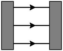
Figure 3: Schematic representation of the $3Q$ normalization. Each quark line stands for the color, flavor and spin contractions $\delta^{\alpha_{i}}_{\alpha^{\prime}_{i}}\delta^{f_{i}}_{f^{\prime}_{i}}\delta^{\sigma_{i}}_{\sigma^{\prime}_{i}}\int\mathrm{d}z^{\prime}_{i}\,\mathrm{d}^{2}\mathbf{p}^{\prime}_{i\perp}\delta(z_{i}-z^{\prime}_{i})\delta^{(2)}(\mathbf{p}_{i\perp}-\mathbf{p}^{\prime}_{i\perp})$.

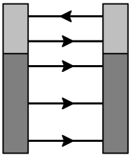
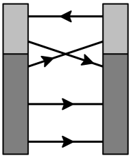
Figure 4: Schematic representation of the $5Q$ direct (left) and exchange (right) contributions to the normalization.

In the $5Q$ sector all contractions are equivalent to either the so-called “direct” diagram or the “exchange” diagram, see Fig.4. In the direct diagram all quarks with the same label are connected while in the exchange one a valence quark is exchanged with the quark of the sea pair. It has appeared in a previous work [9] that exchange diagrams do not contribute much and can thus be neglected. So in the $5Q$ sector we used only the direct contribution in this paper.

The operator acts on each quark line. In the present approach it is then easy to compute separately contribution coming from the valence quarks, the sea quarks or antiquarks, see Fig.5.

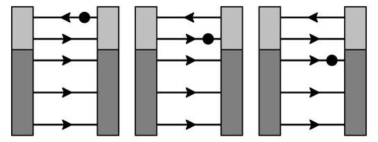
Figure 5: Schematic representation of the three types of $5Q$ contributions to the charges.

These diagrams represent some contraction of color, spin, isospin and flavor indices. For example, the sum of the three diagrams in the $5Q$ sector with the vector current $\bar{\psi}\gamma^{+}\psi$ acting on the quark lines represents the following expression

$$V^{(5)}(1\to 2) = \frac{108}{2}\,\delta^{k}_{l}T(1)^{f_{1}f_{2}f_{3}f_{4},j_{5}}_{j_{1}j_{2}j_{3}j_{4},f_{5},k}T(2)_{f_{1}f_{2}g_{3}g_{4},l_{5}}^{l_{1}l_{2}l_{3}l_{4},g_{5},l}\int(\mathrm{d}p_{1-5})$$ (43)

$$\times F^{j_{1}\sigma_{1}}(p_{1})F^{j_{2}\sigma_{2}}(p_{2})F^{j_{3}\sigma_{3}}(p_{3})W^{j_{4}\sigma_{4}}_{j_{5}\sigma_{5}}(p_{4},p_{5})F^{\dagger}_{l_{1}\sigma_{1}}(p_{1})F^{\dagger}_{l_{2}\sigma_{2}}(p_{2})F^{\dagger}_{l_{3}\tau_{3}}(p_{3})W_{c\,l_{4}\tau_{4}}^{l_{5}\tau_{5}}(p_{4},p_{5})$$

$$\times \left[-\delta^{g_{3}}_{f_{3}}\delta^{g_{4}}_{f_{4}}\boldsymbol{J^{f_{5}}_{g_{5}}}\delta^{\tau_{3}}_{\sigma_{3}}\delta^{\tau_{4}}_{\sigma_{4}}\boldsymbol{\delta_{\tau_{5}}^{\sigma_{5}}}+\delta^{g_{3}}_{f_{3}}\boldsymbol{J^{g_{4}}_{f_{4}}}\delta^{f_{5}}_{g_{5}}\delta^{\tau_{3}}_{\sigma_{3}}\boldsymbol{\delta^{\tau_{4}}_{\sigma_{4}}}\delta_{\tau_{5}}^{\sigma_{5}}+3\boldsymbol{J^{g_{3}}_{f_{3}}}\delta^{g_{4}}_{f_{4}}\delta^{f_{5}}_{g_{5}}\boldsymbol{\delta^{\tau_{3}}_{\sigma_{3}}}\delta^{\tau_{4}}_{\sigma_{4}}\delta_{\tau_{5}}^{\sigma_{5}}\right].$$

6 Scalar overlap integrals

The contractions in the previous section are easily performed by Mathematica over all flavor $(f,g)$, isospin $(j,l)$ and spin $(\sigma,\tau)$ indices. One is then left with scalar integrals over longitudinal $z$ and transverse $\mathbf{p}_{\perp}$ momenta of the quarks. The integrals over relative transverse momenta in the $q\bar{q}$ pair are generally UV divergent. We have chosen to use the Pauli-Villars regularization with mass $M_{\textrm{PV}}=556.8$ MeV (this value being chosen from the requirement that the pion decay constant $F_{\pi}=93$ MeV is reproduced from $M=345$ MeV).

For convenience we introduce the probability distribution $\Phi^{I}(z,\mathbf{q}_{\perp})$ that three valence quarks leave the longitudinal fraction $z=q_{z}/\mathcal{M}$ and the transverse momentum $\mathbf{q}_{\perp}$ to the $q\bar{q}$ pair(s) with $I=V,T$ referring to the vector or tensor case

$$\Phi^{I}(z,\mathbf{q}_{\perp})=\int\mathrm{d}z_{1,2,3}\frac{\mathrm{d}^{2}\mathbf{p}_{1,2,3\perp}}{(2\pi)^{6}}\,\delta(z+z_{1}+z_{2}+z_{3}-1)(2\pi)^{2}\delta^{(2)}(\mathbf{q}_{\perp}+\mathbf{p}_{1\perp}+\mathbf{p}_{2\perp}+\mathbf{p}_{3\perp})D^{I}(p_{1},p_{2},p_{3}).$$ (44)

The function $D^{I}(p_{1},p_{2},p_{3})$ is given in terms of the upper and lower valence wave functions $h(p)$ and $j(p)$ as follows

$$D^{V}(p_{1},p_{2},p_{3}) = h^{2}(p_{1})h^{2}(p_{2})h^{2}(p_{3})+6h^{2}(p_{1})h^{2}(p_{2})\left[h(p_{3})\frac{p_{3z}}{|\mathbf{p}_{3}|}j(p_{3})\right]+3h^{2}(p_{1})h^{2}(p_{2})j^{2}(p_{3})$$ (45)

$$+ 12h^{2}(p_{1})\left[h(p_{2})\frac{p_{2z}}{|\mathbf{p}_{2}|}j(p_{2})\right]\left[h(p_{3})\frac{p_{3z}}{|\mathbf{p}_{3}|}j(p_{3})\right]+12h^{2}(p_{1})\left[h(p_{2})\frac{p_{2z}}{|\mathbf{p}_{2}|}j(p_{2})\right]j^{2}(p_{3})$$

$$+ 8\left[h(p_{1})\frac{p_{1z}}{|\mathbf{p}_{1}|}j(p_{1})\right]\left[h(p_{2})\frac{p_{2z}}{|\mathbf{p}_{2}|}j(p_{2})\right]\left[h(p_{3})\frac{p_{3z}}{|\mathbf{p}_{3}|}j(p_{3})\right]+3h^{2}(p_{1})j^{2}(p_{2})j^{2}(p_{3})$$

$$+ 12\left[h(p_{1})\frac{p_{1z}}{|\mathbf{p}_{1}|}j(p_{1})\right]\left[h(p_{2})\frac{p_{2z}}{|\mathbf{p}_{2}|}j(p_{2})\right]j^{2}(p_{3})+6\left[h(p_{1})\frac{p_{1z}}{|\mathbf{p}_{1}|}j(p_{1})\right]j^{2}(p_{2})j^{2}(p_{3})$$

$$+ j^{2}(p_{1})j^{2}(p_{2})j^{2}(p_{3})$$

$$D^{T}(p_{1},p_{2},p_{3}) = h^{2}(p_{1})h^{2}(p_{2})h^{2}(p_{3})+6h^{2}(p_{1})h^{2}(p_{2})\left[h(p_{3})\frac{p_{3z}}{|\mathbf{p}_{3}|}j(p_{3})\right]+h^{2}(p_{1})h^{2}(p_{2})\frac{p_{3z}^{2}+2p_{3}^{2}}{p_{3}^{2}}j^{2}(p_{3})$$ (46)

$$+ 12h^{2}(p_{1})\left[h(p_{2})\frac{p_{2z}}{|\mathbf{p}_{2}|}j(p_{2})\right]\left[h(p_{3})\frac{p_{3z}}{|\mathbf{p}_{3}|}j(p_{3})\right]+4h^{2}(p_{1})\left[h(p_{2})\frac{p_{2z}}{|\mathbf{p}_{2}|}j(p_{2})\right]\frac{p_{3z}^{2}+2p_{3}^{2}}{p_{3}^{2}}j^{2}(p_{3})$$

$$+ 8\left[h(p_{1})\frac{p_{1z}}{|\mathbf{p}_{1}|}j(p_{1})\right]\left[h(p_{2})\frac{p_{2z}}{|\mathbf{p}_{2}|}j(p_{2})\right]\left[h(p_{3})\frac{p_{3z}}{|\mathbf{p}_{3}|}j(p_{3})\right]+h^{2}(p_{1})j^{2}(p_{2})\frac{2p_{3z}^{2}+rp_{3}^{2}}{p_{3}^{2}}j^{2}(p_{3})$$

$$+ 4\left[h(p_{1})\frac{p_{1z}}{|\mathbf{p}_{1}|}j(p_{1})\right]\left[h(p_{2})\frac{p_{2z}}{|\mathbf{p}_{2}|}j(p_{2})\right]\frac{p_{3z}^{2}+2p_{3}^{2}}{p_{3}^{2}}j^{2}(p_{3})+2\left[h(p_{1})\frac{p_{1z}}{|\mathbf{p}_{1}|}j(p_{1})\right]j^{2}(p_{2})\frac{2p_{3z}^{2}+p_{3}^{2}}{p_{3}^{2}}j^{2}(p_{3})$$

$$+ j^{2}(p_{1})j^{2}(p_{2})\frac{p_{3z}^{2}}{p_{3}^{2}}j^{2}(p_{3}).$$

In the nonrelativistic limit one has $j(p)=0$ and thus $D^{V}(p_{1},p_{2},p_{3})=D^{T}(p_{1},p_{2},p_{3})$. The expression for the axial case can be found in [10].

6.1 $3Q$ scalar integrals

In the $3Q$ sector there is no quark-antiquark pair. There are then two integrals only, $\Phi^{V}(0,0)$ and $\Phi^{T}(0,0)$. Let us remind that in this sector spin-flavor wave functions obtained by the projection technique are equivalent to those given by $SU(6)$ symmetry. One then naturally obtains the same results than given by $SU(6)$ excepted that tensor quantities are multiplied by the factor $\Phi^{T}(0,0)/\Phi^{V}(0,0)$. As discussed earlier this is similar (but not exactly the same) to approaches using Melosh rotations.

6.2 $5Q$ scalar integrals

In the $5Q$ sector there is one quark-antiquark pair and only six integrals are needed. These integrals can be written in the general form

$$K^{I}_{J}=\frac{M^{2}}{2\pi}\int\frac{\mathrm{d}^{3}\mathbf{q}}{(2\pi)^{3}}\,\Phi^{I}\left(\frac{q_{z}}{\mathcal{M}},\mathbf{q}_{\perp}\right)\theta(q_{z})\,q_{z}\,G_{J}(q_{z},\mathbf{q}_{\perp})$$ (47)

where $G_{J}$ is a quark-antiquark probability distribution and $J=\pi\pi,33,\sigma\sigma$. These distributions are obtained by contracting two quark-antiquark wave functions $W$, see eq. (13) and regularized by means of Pauli-Villars procedure

$$G_{\pi\pi}(q_{z},\mathbf{q}_{\perp}) = \Pi^{2}(\mathbf{q})\int^{1}_{0}\mathrm{d}y\int\frac{\mathrm{d}^{2}\mathcal{Q}_{\perp}}{(2\pi)^{2}}\frac{\mathcal{Q}^{2}_{\perp}+M^{2}}{(\mathcal{Q}^{2}_{\perp}+M^{2}+y(1-y)\mathbf{q}^{2})^{2}}-(M\to M_{\textrm{PV}}),$$ (48)

$$G_{33}(q_{z},\mathbf{q}_{\perp}) = \frac{q_{z}^{2}}{\mathbf{q}^{2}}\,G_{\pi\pi}(q_{z},\mathbf{q}_{\perp}),$$ (49)

$$G_{\sigma\sigma}(q_{z},\mathbf{q}_{\perp}) = \Sigma^{2}(\mathbf{q})\int^{1}_{0}\mathrm{d}y\int\frac{\mathrm{d}^{2}\mathcal{Q}_{\perp}}{(2\pi)^{2}}\frac{\mathcal{Q}^{2}_{\perp}+M^{2}(2y-1)^{2}}{(\mathcal{Q}^{2}_{\perp}+M^{2}+y(1-y)\mathbf{q}^{2})^{2}}-(M\to M_{\textrm{PV}}),$$ (50)

where $q_{z}=z\mathcal{M}=(z_{4}+z_{5})\mathcal{M}$ and $\mathbf{q}_{\perp}=\mathbf{p}_{4\perp}+\mathbf{p}_{5\perp}$. There are three integrals in the vector case $K^{V}_{\pi\pi},K^{V}_{33},K^{V}_{\sigma\sigma}$ and three in the tensor one $K^{T}_{\pi\pi},K^{T}_{33},K^{T}_{\sigma\sigma}$. Sea quarks and antiquarks do not contribute to the tensor charge since the the tensor operator is chiral-odd. In this approach it is reflected by the fact that the contraction of two quark-antiquark wave functions $W$ with the tensor operator leaves only vanishing scalar overlap integrals $\int\mathrm{d}^{2}\mathcal{Q}_{\perp}\,\mathcal{Q}_{x}$ or $\int\mathrm{d}^{2}\mathcal{Q}_{\perp}\,\mathcal{Q}_{y}$.

Even though sea quarks and antiquarks do not contribute to the tensor charge it is not sufficient to restrict the computation to the $3Q$ sector where only valence quarks appear. Higher Fock states change the composition of the valence sector as shown by eq. (17). So hidden flavors can access to the valence level and thus contribute to tensor charge of the baryon. In other words, even though only valence quarks contribute $SU(6)$ relations are broken due to relativistic effects (additional quark-antiquark pairs).

7 Results

7.1 Combinatoric results

In this work we have studied tensor charges in flavor $SU(3)$ symmetry. Even though this symmetry is broken in nature, this gives quite a good estimation. The interesting thing is that this symmetry relates tensor charges within each multiplet. Indeed all particles in a given representation are on the same footing and are related through pure flavor $SU(3)$ transformations. One can find the way to relate tensors charges of different members of the same multiplet in [10].

The octet, decuplet and antidecuplet normalizations in the $3Q$ and $5Q$ sectors are given by the following linear combination

$$\mathcal{N}^{(3)}(B_{\bf 8}) = 9\,\Phi^{V}(0,0),$$ (51)

$$\mathcal{N}^{(5)}(B_{\bf 8}) = \frac{18}{5}\left(11K^{V}_{\pi\pi}+23K^{V}_{\sigma\sigma}\right),$$ (52)

$$\mathcal{N}^{(3)}_{3/2}(B_{\bf 10}) = \mathcal{N}^{(3)}_{1/2}(B_{\bf 10})=\frac{18}{5}\,\Phi^{V}(0,0),$$ (53)

$$\mathcal{N}^{(5)}_{3/2}(B_{\bf 10}) = \frac{9}{5}\left(15K^{V}_{\pi\pi}-6K^{V}_{33}+17K^{V}_{\sigma\sigma}\right),$$ (54)

$$\mathcal{N}^{(5)}_{1/2}(B_{\bf 10}) = \frac{9}{5}\left(11K^{V}_{\pi\pi}+6K^{V}_{33}+17K^{V}_{\sigma\sigma}\right),$$ (55)

$$\mathcal{N}^{(5)}(B_{\bf\overline{10}}) = \frac{36}{5}\left(K^{V}_{\pi\pi}+K^{V}_{\sigma\sigma}\right)$$ (56)

where the subscript $3/2,1/2$ refers to the value of third component of the baryon spin $J_{z}$.

Here are the proton tensor charges

$$T^{(3)}_{u}(p) = 12\Phi^{T}(0,0),$$ (57)

$$T^{(3)}_{d}(p) = -3\Phi^{T}(0,0),$$ (58)

$$T^{(3)}_{s}(p) = 0,$$ (59)

$$T^{(5)}_{u}(p) = \frac{18}{25}\left(48K^{T}_{\pi\pi}-7K^{T}_{33}+151K^{T}_{\sigma\sigma}\right),$$ (60)

$$T^{(5)}_{d}(p) = \frac{-12}{25}\left(24K^{T}_{\pi\pi}+19K^{T}_{33}+53K^{T}_{\sigma\sigma}\right),$$ (61)

$$T^{(5)}_{s}(p) = \frac{-12}{25}\left(3K^{T}_{\pi\pi}+8K^{T}_{33}+K^{T}_{\sigma\sigma}\right).$$ (62)

Here are the $\Delta^{++}$ tensor charges

$$T^{(3)}_{u,3/2}(\Delta^{++}) = \frac{54}{5}\Phi^{T}(0,0),$$ (63)

$$T^{(3)}_{d,3/2}(\Delta^{++}) = T^{(3)}_{s,3/2}(B_{\bf 10})=0,$$ (64)

$$T^{(3)}_{u,1/2}(\Delta^{++}) = \frac{18}{5}\Phi^{T}(0,0),$$ (65)

$$T^{(3)}_{d,1/2}(\Delta^{++}) = T^{(3)}_{s,1/2}(\Delta^{++})=0,$$ (66)

$$T^{(5)}_{u,3/2}(\Delta^{++}) = \frac{9}{10}\left(56K^{T}_{\pi\pi}-17K^{T}_{33}+101K^{T}_{\sigma\sigma}\right),$$ (67)

$$T^{(5)}_{d,3/2}(\Delta^{++}) = T^{(5)}_{s,3/2}(B_{\bf 10})=\frac{-9}{20}\left(8K^{T}_{\pi\pi}+13K^{T}_{33}-K^{T}_{\sigma\sigma}\right),$$ (68)

$$T^{(5)}_{u,1/2}(\Delta^{++}) = \frac{3}{10}\left(42K^{T}_{\pi\pi}+25K^{T}_{33}+101K^{T}_{\sigma\sigma}\right),$$ (69)

$$T^{(5)}_{d,1/2}(\Delta^{++}) = T^{(5)}_{s,1/2}(\Delta^{++})=\frac{-3}{20}\left(6K^{T}_{\pi\pi}+19K^{T}_{33}-K^{T}_{\sigma\sigma}\right).$$ (70)

Here are the $\Theta^{+}$ tensor charges

$$T^{(5)}_{u}(\Theta^{+}) = T^{(5)}_{d}(\Theta^{+})=\frac{-18}{5}\left(K^{T}_{33}-K^{T}_{\sigma\sigma}\right),$$ (71)

$$T^{(5)}_{s}(\Theta^{+}) = 0.$$ (72)

In the $5Q$ sector of $\Theta^{+}$ pentaquark the strange flavor appears only as an antiquark as one can see from its minimal quark content $uudd\bar{s}$. That’s the reason why we have found no strange contribution. But if at least the $7Q$ sector was considered we would have obtained a nonzero contribution due flavor components like $|uus(d\bar{s})(d\bar{s})\rangle$, $|uds(u\bar{s})(d\bar{s})\rangle$ and $|dds(u\bar{s})(u\bar{s})\rangle$.

7.2 Numerical results

In the evaluation of the scalar integrals we have used the constituent quark mass $M=345$ MeV, the Pauli-Villars mass $M_{\textrm{PV}}=556.8$ MeV for the regularization of (48)-(50) and the baryon mass $\mathcal{M}=1207$ MeV as it follows for the “classical” mass in the mean field approximation [25]. Choosing $\Phi^{V}(0,0)=1$ we have obtained in the $3Q$ sector

$$\Phi^{T}(0,0)=0.9306$$ (73)

and in the $5Q$ sector

$$K^{V}_{\pi\pi}=0.0365,\qquad K^{V}_{33}=0.0197,\qquad K^{V}_{\sigma\sigma}=0.0140,$$ (74)

$$K^{T}_{\pi\pi}=0.0333,\qquad K^{T}_{33}=0.0180,\qquad K^{T}_{\sigma\sigma}=0.0126.$$ (75)

This has to be compared with the results in the axial case [9]

$$\Phi^{A}(0,0)=0.8612$$ (76)

$$K^{A}_{\pi\pi}=0.0300,\qquad K^{A}_{33}=0.0163,\qquad K^{A}_{\sigma\sigma}=0.0112.$$ (77)

As expected from (40), (41) and (42) we have the following pattern for the integrals $|V|>|T|>|A|$.

7.3 Discussion

We collect in Tables 1, 2 and 3 our results concerning the tensor charges at the model scale $Q_{0}^{2}=0.36$ GeV².

Table 1: Our proton tensor charges and their isovector and isoscalar combinations.

$p^{+}$	$\delta u$	$\delta d$	$\delta s$	$g_{T}^{(3)}$	$g_{T}^{(0)}$
$3Q$	1.241	-0.310	0	1.551	0.931
$3Q+5Q$	1.172	-0.315	-0.011	1.487	0.846

Table 2: Our $\Delta^{++}$ tensor charges and their isovector and isoscalar combinations.

$\Delta^{++}_{3/2}$	$\delta u$	$\delta d$	$\delta s$	$g_{T}^{(3)}$	$g_{T}^{(0)}$
$3Q$	2.792	0	0	2.792	2.792
$3Q+5Q$	2.624	-0.046	-0.046	2.670	2.532
$\Delta^{++}_{1/2}$	$\delta u$	$\delta d$	$\delta s$	$g_{T}^{(3)}$	$g_{T}^{(0)}$
$3Q$	0.931	0	0	0.931	0.931
$3Q+5Q$	0.863	-0.016	-0.016	0.879	0.831

Table 3: Our $\Theta^{+}$ tensor charges and their isovector and isoscalar combinations.

$\Theta^{+}$	$\delta u$	$\delta d$	$\delta s$	$g_{T}^{(3)}$	$g_{T}^{(0)}$
$3Q+5Q$	-0.053	-0.053	0	0	-0.107

Like all other models for the proton $\delta u$ and $\delta d$ are not small and have a magnitude similar to $\Delta u$ and $\Delta d$. One can also check that Soffer’s inequality (21) is satisfied for explicit flavors. However hidden flavors, i.e. $s$ in proton and $d,s$ in $\Delta^{++}$, violate the inequality.

Up to now only one experimental extraction of transversity distributions has been achieved [26]. The authors did not give explicit values for tensor charges. They have however been estimated to $\delta u=0.46^{+0.36}_{-0.28}$ and $\delta d=-0.19^{+0.30}_{-0.23}$ in [16] at the scale $Q^{2}=0.4$ GeV². These values are unexpectedly small compared to models predictions. Further experimental results are then highly desired to either confirm or infirm the smallness of tensor charges.

8 Conclusion

We have used Chiral Quark Soliton Model ($\chi$QSM) formulated in the Infinite Momentum Frame (IMF) up to $5Q$ Fock component to investigate octet, decuplet and antidecuplet tensor charges. We have obtained $\delta u=1.172$ and $\delta d=-0.315$ at $Q_{0}^{2}=0.36$ GeV² for the proton which are in the range of prediction of the other models.

We have also discussed the Melosh rotations involved in usual light-cone approach compared with our approach. Melosh rotation introduces somewhat artificially angular momentum whose origin is purely kinematical. A general light-cone wave function should in fact contain a dynamical term like in the approach used in this paper.

Usual light-cone models consider only the $3Q$ sector and thus cannot estimate the strange tensor charge $\delta s$. Even though sea quarks and antiquarks do not contribute to tensor charges one can obtain a nonzero $\delta s$ because the $5Q$ component of the nucleon allows strange quarks to access to the valence level. Our result is $\delta s=-0.011$ and thus a negative transverse polarisation of strange quarks.

Acknowledgements

The author is grateful to RUB TP2 for its kind hospitality and to M. Polyakov for his careful reading and comments. The author is also indebted to J. Cugnon whose absence would not have permitted the present work to be done. This work has been supported by the National Funds of Scientific Research, Belgium.

References

• [1] J. Ralston and D.E. Soper, Nucl. Phys. B152 (1979) 109.
• [2] R.L. Jaffe and X. Ji, Phys. Rev. Lett. 67 (1991) 552.
• [3] R.L. Jaffe and X. Ji, Nucl. phys. B375 (1992) 527.
• [4] J. Collins, Nucl. Phys. B394 (1993) 169.
• [5] V. Barone, A. Drago and P.G. Ratcliffe, Phys. Rept. 359 (2002) 1, hep-ph/0104283.
• [6] D. Diakonov and V. Petrov, JETP Lett. 43 (1986) 57 [Pisma Zh. Eksp. Teor. Fiz. 43 (1986) 57];
D. Diakonov, V. Petrov and P. Pobylitsa, Nucl. Phys. B306 (1988) 809;
D. Diakonov and V. Petrov, in Handbook of QCD, ed. M. Shifman, World Scientific, Singapore (2001), vol. 1, p. 359, hep-ph/0009006.
• [7] V. Petrov and M. Polyakov, hep-ph/0307077.
• [8] D. Diakonov and V. Petrov, Phys. Rev. D72 (2005) 074009, hep-ph/0505201.
• [9] C. Lorcé, Phys. Rev. D74 (2006) 054019, hep-ph/0603231.
• [10] C. Lorcé, arXiv:0708.3139.
• [11] B.L. Ioffe and A. Khodjamirian, Phys. Rev. D51 (1995) 33.
• [12] V. Barone, T. Calarco and A. Drago, Phys. Lett. B390 (1997) 287.
• [13] H.-C. Kim, M.V. Polyakov and K. Goeke, Phys. Lett. 387 (1996) 577; P.V. Pobylitsa and M.V. Polyakov, Phys. Lett. B389 (1996) 350.
• [14] I. Schmidt and J. Soffer, Phys. Lett. B407 (1997) 331.
• [15] L. Gamberg and G.R. Goldstein, hep-ph/0106178;
L. Gamberg and G.R. Goldstein, Phys. Rev. Lett. 87 (2001) 242001.
• [16] I.C. Cloët, W. Bentz and A.W. Thomas, arXiv:0708.3246.
• [17] J. Soffer, Phys. Rev. Lett. 74 (1995) 1292.
• [18] J. Soffer, R.L. Jaffe and X. Ji, Phys. Rev. D52 (1995) 5006.
• [19] H.J. Melosh, Phys. Rev. D9 (1974) 1095.
• [20] B.-Q. Ma, J. Phys. G17 (1991) L53;
B.-Q. Ma and Q.-R. Zhang, Z. Phys. C58 (1993) 479.
• [21] S.J. Brodsky and F. Schlumpf, Phys. Lett. B329 (1994) 111.
• [22] S.J. Brodsky, J.R. Hiller, D.S. Hwang and V.A. Karmanov, Phys. Rev. D69 (2004) 076001, hep-ph/0311218.
• [23] S.D. Drell and T.M. Yan, Phys. Rev. Lett. 24 (1970) 181.
• [24] S.J. Brodsky, H.C. Pauli and S.S. Pinsky, Phys. Rep. 301 (1998) 299-486.
• [25] D. Diakonov, V. Petrov and M. Praszalowicz, Nucl. Phys. B323 (1989) 53.
• [26] M. Anselmino, M. Boglione, U. D’Alesio, A. Kotzinian, F. Murgia, A. Prokudin and C. Turk, Phys. Rev. D75 (2007) 054032, hep-ph/0701006.