Constraining Dark Energy and Cosmological Transition Redshift with Type Ia Supernovae

Abstract

The property of dark energy and the physical reason for acceleration of the present universe are two of the most difficult problems in modern cosmology. The dark energy contributes about two-thirds of the critical density of the present universe from the observations of type-Ia supernova (SNe Ia) and anisotropy of cosmic microwave background (CMB).The SN Ia observations also suggest that the universe expanded from a deceleration to an acceleration phase at some redshift, implying the existence of a nearly uniform component of dark energy with negative pressure. We use the “gold” sample containing 157 SNe Ia and two recent well-measured additions, SNe Ia 1994ae and 1998aq to explore the properties of dark energy and the transition redshift. For a flat universe with the cosmological constant, we measure $\Omega_{M}=0.28_{-0.05}^{+0.04}$, which is consistent with Riess et al. The transition redshift is $z_{T}=0.60_{-0.08}^{+0.06}$. We also discuss several dark energy models that define the $w(z)$ of the parameterized equation of state of dark energy including one parameter and two parameters ($w(z)$ being the ratio of the pressure to energy density). Our calculations show that the accurately calculated transition redshift varies from $z_{T}=0.29_{-0.06}^{+0.07}$ to $z_{T}=0.60_{-0.08}^{+0.06}$ across these models. We also calculate the minimum redshift $z_{c}$ at which the current observations need the universe to accelerate.

1 Introduction

Type Ia Supernovae (SNe Ia) have been considered astronomical standard candles and used to measure the geometry and dynamics of the universe. Kowal (1968) showed that SNe Ia give a well-defined Hubble diagram whose intercept could provide a good measurement of the Hubble constant. Colgate (1979) suggested that the peak luminosity $L_{p}$ is a constant. Subsequent observations showed that Type-I SNe should be split (Uomoto & Kirshier 1985; Porter & Filippenko 1987). Theoretical models suggested that SNe Ia arise from the thermonuclear explosion of a carbon-oxygen white dwarf when its mass reaches the Chandrasekhar mass (Colgate & McKee 1969). Colgate (1979) suggested that observations of SNe Ia around $z\simeq 1$ could measure the deceleration parameter $q_{0}$. Hansen, Jrgensen & N$\o$rgaard-Nielsen (1987) detected SN 1988U at $z=0.31$. At this redshift 100 SNe Ia would have been needed to distinguish between an open and a closed universe. Phillips (1993) discovered the intrinsic relation in SNe Ia: $L_{p}=a\times\bigtriangleup{m}_{15}^{b}$, where $\bigtriangleup{m}_{15}$ is the decline rate in the optical band 15 days after the peak luminosity. This relation could be used to explore cosmology.

Using 16 high-redshift SNe and 34 nearby SNe, Riess et al. (1998) found that our universe has been accelerating. Using 42 SNe Ia, Perlmutter et al. (1999) obtained the same result. SN Ia observations also provided evidence for a decelerating universe at redshifts higher than the transition redshift $z_{T}\simeq 0.5$ (Riess et al. 2001; Turner et al. 2002; Riess et al. 2004). Tonry et al. (2003) found that $\Omega_{M}=0.28\pm 0.05$ and $-1.48<w<-0.72$ at the 95% confidence level for a flat universe from high-$z$ SNe. Daly & Djorgovski (2003) derived that the universe changed from deceleration to acceleration at $z_{T}=0.45$ using a model-independent method. Combining the constraints from the recent Ly- forest analysis of Sloan Digital Sky Survey (SDSS) and the SDSS galaxy bias analysis with previous constraints from the SDSS galaxy clustering, the latest SNe, and first-year WMAP cosmic microwave background anisotropies, Seljak et al. (2004) found that $\Omega_{\Lambda}=0.72\pm 0.02$, $w(z=0.3)=-0.98_{-0.12}^{+0.10}$. In the model of $w(z)=w_{0}$, they found $w_{0}=-0.990_{-0.093-0.201-0.351}^{+0.086+0.160+0.222}(1\sigma,2\sigma,3\sigma)$ . From their analysis they concluded that the equation of state did not vary with redshift. Alam et al. (2004) obtained the transition redshift $z_{T}=0.57\pm 0.07$ from a joint analysis of SNe Ia and CMB. Utilizing SNe Ia data, Bassett et al. (2004) derived that the transition redshift varied from $z_{T}=0.14$ to $z_{T}=0.59$, but Gong (2004) found $z_{T}\simeq 0.3$. Jarvis et al (2005) analysized the 75 square degree CTIO lensing survey in conjunction with CMB and SN Ia data and measured $w_{0}=-0.894_{-0.208}^{+0.156}(95\%confidencelevel)$. When taking the dark energy model of $w(a)=w_{0}+w_{a}(1-a)$, they found $w_{0}=-1.19_{-1.74}^{+0.53},w_{a}=1.31_{-2.40}^{+3.04}(95\%confidencelevel)$. Gong (2005) found the transition redshift was $z_{T}\simeq 0.6$ using one-parameter dark energy models. Chang et al. (2005) gave $w_{0}=-1.29$, the deceleration parameter $q_{0}=-0.97$ and $z_{T}=0.70$ by using the recent data of X-ray cluster gas mass fraction. Clocchiatti et al. (2005) derived $\Omega_{M}=0.79^{+0.15}_{-0.18}$ and $\Omega_{\Lambda}=1.57^{+0.24}_{-0.32}$ ($1\sigma$ confidence level) if no prior assumption is made, or $\Omega_{M}=0.29^{+0.06}_{-0.05}$ if $\Omega_{M}+\Omega_{\Lambda}=1$ is assumed, from a sample of 75 low-redshift and 47 high-redshift SNe Ia with the MLCS2k2 luminosity calibration. For a different sample of 58 low-redshift and 48 high-redshift SNe Ia with luminosity calibrations using the PRES method, the results were $\Omega_{M}=0.43^{+0.17}_{-0.19}$ and $\Omega_{\Lambda}=1.18^{+0.27}_{-0.28}$ ($1\sigma$ confidence level) on no prior assumptions, or $\Omega_{M}=0.18^{+0.05}_{-0.04}$ if $\Omega_{M}+\Omega_{\Lambda}=1$ was assumed. Virey et al. (2005) argued that the determi ation of the present deceleration parameter $q_{0}$ through a simple kinematical description could lead to wrong conclusions. A dynamical dark energy model must be taken into account. Meng & Fan (2005) suggested that LAMOST redshift survey could help to reduce the error bounds of dark energy parameters expected from other observations. Zhang & Wu (2005) derived a transition redshift of $z_{T}=0.63$ using the CMB, LSS and SNe Ia data for the holographic dark energy model.

Riess et al.(2004) selected a sample of 157 well-measured SNe Ia, called the “gold” sample. Assuming a flat universe, they concluded: (1) Using the strong prior of $\Omega_{M}=0.27\pm 0.04$, fitting to a static dark energy equation of state yields $-1.46<w<-0.78$ (95% confidence level). (2) Assuming a possible redshift dependence of $w(z)$ (e.g., using $w(z)=w_{0}+w_{1}z$), the data with the strong prior indicate that the region $w_{1}<0$ and especially the quadrant ($w_{0}>-1$ and $w_{1}<0$) are the least favored. (3) Expand $q(z)$ into two terms: $q(z)=q_{0}+zdq/dz$. If the transition redshift is defined through $q(z_{T})=0$, they found $z_{T}=0.46\pm 0.13$.

Currently SN Ia observations provide the most direct way to probe the dark energy component at low redshifts. This is due to the fact that SN data allows a direct measure of the luminosity distance, which is directly related to the expansion law of the universe. Since 1998, many dark energy models have been proposed in the literature. The simplest one is that dark energy is constant, $w(z)=w_{0}$. A linear parameterization is $w(z)=w_{0}+w_{1}z$. Recently a simple two-parameter model $w(z)=w_{0}+w_{1}z/(1+z)$ was discussed. By fitting the model to SNe Ia data, $w_{0}+w_{1}>0$ was found. At high redshifts, however, this model was not valid. In order to solve the problem, Jassal, Bagla & Padmanabhan (2004) modified this parameterization to $w(z)=w_{0}+w_{1}z/(1+z)^{2}$. Hannestad & Mörtsell (2004) parameterized $w_{z}$ as $w_{z}=[1+\big{(}\frac{1+z}{1+z_{s}}\big{)}^{q}]/[w_{o}^{-1}+w_{1}^{-1}(\frac{1+z}{1+z_{s}}\big{)}^{q}]$ . The equation of state $w(z)$ was parametrized by Lee (2005) as $w_{z}=w_{r}\times[w_{0}\exp(qx)+\exp(qx_{c})]/[\exp(qx)+\exp(qx_{c})]$, where $x=\ln a=-\ln(1+z)$. Johri & Rath (2005) found all the observational constraints are satisfied by the two above parameterizations by the combined CMB, LSS and SN Ia data. The Hannestad-Mörtsell model and the Lee four-parameter model for the equation of state may be well-behaved representations of dark energy evolution in a large range of redshifts. Here we examine two phenomenological parametrizations for the variable dark energy which were given by Wetterich (2004).

In our MNRAS paper, we used gamma-ray bursts and 157 SNe Ia to constrain cosmological parameters and transition redshift in only four dark energy models. In this paper, we systematically explore the properties of dark energy and cosmological transition redshift in several dark energy models. The structure of this paper is as follows: In Section 2, we describe our analysis methods and numerical results in a Friedmann-Robertson-Walker cosmology with the cosmological constant. In Section 3, we present cosmological constraints in the one-parameter dark-energy models. In Section 4, we explore the cosmological constraints in two-parameter dark-energy models. Conclusions and a brief discussion are presented in Section 5.

2 cosmology with the cosmological constant

The SN Ia observations provide the currently most direct way of probing the dark energy at low to medium redshifts since the luminosity-distance relation is directly related to the expansion history of the universe. The luminosity distance is given by (Dicus & Repko 2004)

$$d_{L}=\left\{\begin{array}[]{l}\displaystyle cH_{0}^{-1}(1+z)(-\Omega_{k})^{-1/2}\sin((-\Omega_{k})^{1/2}I)\phantom{sssssssssssssssss}\Omega_{k}<0,\\ \displaystyle cH_{0}^{-1}(1+z)I\phantom{ssssssssssssssssssssssssssssssssssssssss}\Omega_{k}=0,\\ \displaystyle cH_{0}^{-1}(1+z)(\Omega_{k})^{-1/2}\sinh((\Omega_{k})^{1/2}I)\phantom{ssssssssssssssssssss}\,\Omega_{k}>0,\\ \end{array}\right.$$ (1)

where

$$\Omega_{k}=1-\Omega_{M}-\Omega_{DE},$$ (2)

$$I=\int_{0}^{z}dz/H(z),$$ (3)

$$H(z)=((1+z)^{3}\Omega_{M}+f(z)\Omega_{DE}+(1+z)^{2}\Omega_{k})^{1/2},$$ (4)

$$f(z)=\exp[3\int_{0}^{z}\frac{(1+w(z^{\prime}))dz^{\prime}}{(1+z^{\prime})}],$$ (5)

where $w(z)$ is the equation of state for dark energy and $d_{L}$ is the luminosity distance. The luminosity distance expected in a Friedmann-Robertson-Walker (FRW) cosmology with mass density $\Omega_{k}$ and vacuum energy density (i.e., the cosmological constant) $\Omega_{\Lambda}$ is

$$d_{L} = c(1+z)H_{0}^{-1}|\Omega_{k}|^{-1/2}{\rm sinn}\{|\Omega_{k}|^{1/2}$$ (6)

$$\times\int_{0}^{z}dz[(1+z)^{2}(1+\Omega_{M}z)-z(2+z)\Omega_{\Lambda}]^{-1/2}\},$$

where $\Omega_{k}=1-\Omega_{M}-\Omega_{\Lambda}$, and $\rm sinn$ is $\sinh$ for $\Omega_{k}>0$ and $\sin$ for $\Omega_{k}<0$ (Carroll et al. 1992). For $\Omega_{k}=0$, the luminosity distance is $d_{L}=cH_{0}^{-1}(1+z)$ times the integral. With $d_{L}$ in units of megaparsecs, the predicted distance modulus is

$$\mu=5\log(d_{L})+25.$$ (7)

We can plot the Hubble diagram for the Gold sample containing 157 SNe Ia and two recent, well-measured SNe Ia 1994ae and 1998aq (Riess et al. 2005). The likelihood functions for the parameters $\Omega_{M}$ and $\Omega_{\Lambda}$ can be determined from $\chi^{2}$ statistic,

$$\chi^{2}(H_{0},\Omega_{M},\Omega_{\Lambda})=\sum_{i=1}^{N}\frac{[\mu_{i}(z_{i},H_{0},\Omega_{M},\Omega_{\Lambda})-\mu_{0,i}]^{2}}{\sigma_{\mu_{0,i}}^{2}+\sigma_{\nu}^{2}},$$ (8)

where $\sigma_{\nu}$ is the dispersion in the supernova redshift (transformed to distance modulus) due to peculiar velocities, and $\sigma_{\mu_{0,i}}$ is the uncertainty in the individual distance moduli. The confidence regions in the $\Omega_{M}-\Omega_{\Lambda}$ plane can be found through marginalizing the likelihood functions over $H_{0}$ (i.e., integrating the probability density $p\propto\exp^{-\chi^{2}/2}$ for all values of $H_{0}$). The Friedmann equations are

$$H^{2}+\frac{k}{a^{2}}=\frac{8\pi G}{3}(\rho_{M}+\rho_{r}+\rho),$$ (9)

$$\dot{\rho}+3H(\rho+p)=0.$$ (10)

The Hubble constant $H=\dot{a}/a$, the dot representing time derivative. Here $\rho$ is defined as

$$\rho=\rho_{0}\exp[3\int_{0}^{z}\frac{(1+w(z^{\prime}))dz^{\prime}}{(1+z^{\prime})}].$$ (11)

$\rho_{M}$ is the matter energy density, $\rho_{r}$ the radiation energy density and $z=a_{0}/a-1$ is the redshift. Combining equations (9) and (10), we can find the acceleration equation,

$$\frac{\ddot{a}}{a}=-\frac{4\pi G}{3}(\rho_{M}+2\rho_{r}+\rho+3p).$$ (12)

At $\ddot{a}=0$, the universe changes from deceleration to acceleration phase. So we can define the transition redshift. For the cosmological-constant model we obtain the transition redshift,

$$z_{T}=(\frac{2\Omega_{\Lambda}}{\Omega_{M}})^{1/3}-1.$$ (13)

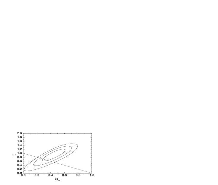
Figure 2: Left panel shows the $1\sigma$, $2\sigma$, $3\sigma$ confidence levels in the $\Omega_{M}-\Omega_{\Lambda}$ plane. The line represents the flat universe. Right panel shows the transition redshift probability curve. The transition redshift can be summarily expressed by $z_{T}=0.60_{-0.08}^{+0.06}$.

In Figure 1 we plot the Hubble diagram for the 159 SNe Ia. We use the 159 SNe Ia data to obtain the confidence regions and transition redshift (see Fig. 2). For a flat universe, we obtain $\Omega_{M}=0.28_{-0.05}^{+0.04}$. This result is consistent with Riess et al. (2004). The best value for the transition redshift is $z_{T}=0.60_{-0.08}^{+0.06}$. Let $z_{c}$ be the minimum redshift at which current observations require the universe to accelerate; it is determined from the condition $d(t_{c},t_{0})=1/H(t_{c})$. So we have

$$\int_{0}^{z_{c}}\frac{dz}{\sqrt{\Omega_{M}(1+z)^{3}+\Omega_{\Lambda}(1+z)^{3(1+w)}}}=\frac{1+z_{c}}{\sqrt{{\Omega_{M}(1+z_{c})^{3}+\Omega_{\Lambda}(1+z_{c})^{3(1+w)}}}}.$$ (14)

With a prior of $\Omega_{M}=0.27\pm 0.04$, we get $z_{c}=2.01>z_{T}=0.60$.

3 One-parameter dark-energy model

3.1 Constant parameterization

We consider an equation of state for dark energy,

$$w_{z}=w_{0}.$$ (15)

In this dark energy model, the luminosity distance for a flat universe is (Riess et al. 2004)

$$d_{L}=cH_{0}^{-1}(1+z)\int_{0}^{z}dz[(1+z)^{3}\Omega_{M}+(1-\Omega_{M})(1+z)^{3(1+w_{0})}]^{-1/2}.$$ (16)

Combining equations (11), (12) and (15), we calculate the transition redshift through

$$\Omega_{M}+(1-\Omega_{M})(1+3w_{0})\times(1+z)^{3w_{0}}=0.$$ (17)

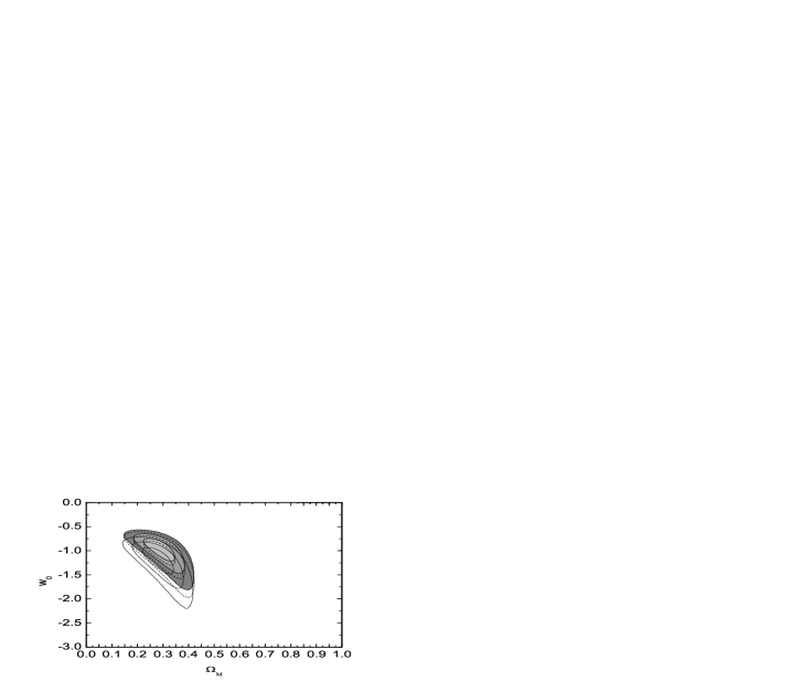
Figure 3: Left panel shows the $1\sigma$, $2\sigma$, $3\sigma$ confidence regions in the $\Omega_{M}-w_{0}$ plane. Grey contours refer to the $w_{z}=w_{0}$ model; dashed contours, the $w_{z}=\frac{w_{0}}{1+z}\exp(\frac{z}{1+z})$ model; dotted contours, to the $w_{z}=\frac{w_{0}}{1+z}$ model. Right panel shows the transition redshift probability curve. Dotted, dashed and full lines refer respectively to the $w_{z}=w_{0}$ model the $w_{z}=\frac{w_{0}}{1+z}\exp(\frac{z}{1+z})$ model, and the $w_{z}=\frac{w_{0}}{1+z}$ model.

We use the 159 SNe Ia data to obtain the confidence regions and transition redshift, and derive $w_{0}=-0.975_{-0.15}^{+0.12}$ at the $1\sigma$ confidence level. See Figure 3. So if we assume $w_{0}=\rm constant$, then the SN Ia data favor $w_{0}=-1$. At the 95% confidence level we have $-1.35<w_{0}<-0.75$. These results are consistent with Tonry et al. (2003), Knop et al. (2003), Bennett et al. (2003), Riess et al. (2004). The best value of the transition redshift is $z_{T}=0.52_{-0.06}^{+0.05}(1\sigma)$. In this dark energy model $z_{c}$ satisfies the following equation,

$$\int_{0}^{z_{c}}\frac{dz}{\sqrt{\Omega_{M}(1+z)^{3}+(1-\Omega_{M})(1+z)^{3(1+w_{0})}}}$$

$$=\frac{1+z_{c}}{\sqrt{{\Omega_{M}(1+z_{c})^{3}+(1-\Omega_{M})(1+z_{c})^{3(1+w_{0})}}}}.$$ (18)

For $\Omega_{M}=0.27$ and $w_{0}=-0.975$, we get $z_{c}=2.02>z_{T}=0.52$.

We now consider the second one-parameter dark energy equation (Gong & Zhang 2005),

$$w_{z}=\frac{w_{0}}{1+z}\exp(\frac{z}{1+z}).$$ (19)

In this model the luminosity distance is given by

$$d_{L}=cH_{0}^{-1}(1+z)\int_{0}^{z}dz[(1+z)^{3}\Omega_{M}+(1-\Omega_{M})(1+z)^{3}\exp(3w_{0}e^{\frac{z}{1+z}}-3w_{0})]^{-1/2}.$$ (20)

Combining equations (11), (12) and (19), we can calculate the transition redshift through

$$\Omega_{M}+(1-\Omega_{M})(1+\frac{3w_{0}}{1+z}e^{z/(1+z)})\times\exp(3w_{0}(e^{z/(1+z)}-1))=0.$$ (21)

Again we use the 159 SNe Ia data to obtain confidence regions and transition redshift and derive $w_{0}=-1.10_{-0.11}^{+0.16}$ at the $1\sigma$ confidence level, shown in Figure 3. We obtain $-1.32<w_{0}<-0.76$ at the 95% confidence level. The transition redshift is found to be $z_{T}=0.47^{+0.07}_{-0.05}(1\sigma)$. In this dark energy model. $z_{c}$ satisfies the following equation,

$$\int_{0}^{z_{c}}\frac{dz}{\sqrt{(1+z)^{3}\Omega_{M}+(1-\Omega_{M})(1+z)^{3}\exp(3w_{0}e^{\frac{z}{1+z}}-3w_{0})}}$$

$$=\frac{1+z_{c}}{\sqrt{(1+z_{c})^{3}\Omega_{M}+(1-\Omega_{M})(1+z_{c})^{3}\exp(3w_{0}e^{\frac{z_{c}}{1+z_{c}}}-3w_{0})}}.$$ (22)

For $\Omega_{M}=0.27$ and $w_{0}=-1.10$, we get $z_{c}=1.90>z_{T}=0.47$.

Our third one-parameter dark energy model (Gong & Zhang 2005), is

$$w_{z}=\frac{w_{0}}{1+z}.$$ (23)

Proceeding as before, we obtain the luminosity distance

$$d_{L}=cH_{0}^{-1}(1+z)\int_{0}^{z}dz[(1+z)^{3}\Omega_{M}+(1-\Omega_{M})(1+z)^{3}e^{(\frac{3w_{0}z}{1+z})}]^{-1/2}.$$ (24)

Combining equations (11), (12) and (23), we calculate the transition redshift through

$$\Omega_{M}+(1-\Omega_{M})(1+\frac{3w_{0}}{1+z})\times\exp{(\frac{3w_{0}z}{1+z})}=0.$$ (25)

Again for the 159 SNe Ia data the confidence regions and transition redshift are obtained. We have $w_{0}=-1.15_{-0.17}^{+0.20}$ at the $1\sigma$ confidence level shown in Figure 3 and derive $-1.37<w_{0}<-0.78$ at the 95% confidence level. The transition redshift is $z_{T}=0.49^{+0.06}_{-0.05}(1\sigma)$. In this dark energy model $z_{c}$ satisfies the following equation,

$$\int_{0}^{z_{c}}\frac{dz}{\sqrt{\Omega_{M}(1+z)^{3}+(1-\Omega_{M})(1+z)^{3}e^{(\frac{3w_{0}z}{1+z})}}}$$

$$=\frac{1+z_{c}}{\sqrt{\Omega_{M}(1+z_{c})^{3}+(1-\Omega_{M})(1+z)^{3}e^{(\frac{3w_{0}z_{c}}{1+z_{c}})}}}.$$ (26)

For $\Omega_{M}=0.27$ and $w_{0}=-1.15$, we obtain $z_{c}=1.63>z_{T}=0.49$.

4 Two-parameter dark-energy model

4.1 Wetterich’s parameterization

In this section, we first consider the dark energy parameterization proposed by Wetterich (Wetterich 2004):

$$w_{z}=\frac{w_{0}}{[1+b\ln(1+z)]^{2}}.$$ (27)

In this model the luminosity distance is given by

$$d_{L}=cH_{0}^{-1}(1+z)\int_{0}^{z}dz[(1+z)^{3}\Omega_{M}+(1-\Omega_{M})(1+z)^{3+3w_{0}/[1+b\ln(1+z)]}]^{-1/2}.$$ (28)

Using the above method we calculate the transition redshift through

$$\Omega_{M}+(1-\Omega_{M})(1+\frac{3w_{0}}{[1+b\ln(1+z)]^{2}})\times(1+z)^{3+3w_{0}/[1+b\ln(1+z)]}=0.$$ (29)

We consider a Gaussian prior of $\Omega_{M}=0.27\pm 0.04$. We plot the transition redshift probability curve. The transition redshift is $z_{T}=0.39_{-0.05}^{+0.06}(1\sigma)$ in Figure 4, but Gong (2004) obtained $z_{T}=0.26$, which is somewhat smaller than our result. This may be caused by differences in the calculation method and data.

Because the best fit for the above parameterization gives $\Omega_{M}\sim 0$ which is not physical, we apply a modified Wetterich’s parameterization (Gong 2004)

$$w_{z}=\frac{w_{0}}{1+b\ln(1+z)}.$$ (30)

Combining Equations (1)–(5) and (30), the luminosity Distance is calculated with,

$$d_{L}=cH_{0}^{-1}(1+z)\int_{0}^{z}dz[(1+z)^{3}\Omega_{M}+(1-\Omega_{M})(1+z)^{3}[1+b\ln(1+z)]^{3w_{0}/b}]^{-1/2}.$$ (31)

Following the above method, we calculate the transition redshift through

$$\Omega_{M}+(1-\Omega_{M})(1+\frac{3w_{0}}{[1+b\ln(1+z)]})\times[1+b\ln(1+z)]^{3w_{0}/b}=0.$$ (32)

We use a Gaussian prior of $\Omega_{M}=0.27\pm 0.04$. The transition shift probability curve is plotted. The transition redshift is $z_{T}=0.29_{-0.06}^{+0.07}(1\sigma)$ in Figure 4. This result is consistent with Gong (2004).

We consider another modified Wetterich’s parameterization:

$$w_{z}=w_{0}+\frac{w_{1}}{1+\ln(1+z)}.$$ (33)

Combining equations (1)-(5) and (33), we can obtain the luminosity distance with,

$$d_{L}=cH_{0}^{-1}(1+z)\int_{0}^{z}dz[(1+z)^{3}\Omega_{M}+(1-\Omega_{M})(1+z)^{3+3w_{0}}[1+\ln(1+z)]^{3w_{1}}]^{-1/2}.$$ (34)

Using the above method, we calculate the transition redshift through

$$\Omega_{M}+(1-\Omega_{M})(1+3w_{0}+\frac{3w_{1}}{1+\ln(1+z)})\times(1+z)^{3w_{0}}[1+\ln(1+z)]^{3w_{1}}=0.$$ (35)

We use a Gaussian prior of $\Omega_{M}=0.27\pm 0.04$. The transition redshift probability curve is plotted. The transition redshift is $z_{T}=0.42_{-0.07}^{+0.06}(1\sigma)$ in Figure 4, but Gong (2004) obtained $z_{T}=0.34$, which is slightly smaller than our result. This may be caused by differences in the calculation method and data.

4.2 Linder’s parameterization

The simplest parameterization including two parameters is (Maaor et al. 2001; Weller &Albrecht 2001; Weller &Albrecht 2002; Riess et al. 2004),

$$w_{z}=w_{0}+w_{1}z.$$ (36)

This parameterization provides the minimum possible resolving power to distinguish between the cosmological constant and time-dependent dark energy. We again use the above method to calculate the luminosity distance with,

$$d_{L}=cH_{0}^{-1}(1+z)\int_{0}^{z}dz[(1+z)^{3}\Omega_{M}+(1-\Omega_{M})(1+z)^{3(1+w_{0}-w_{1})}e^{3w_{1}z}]^{-1/2}.$$ (37)

Combining equations (11), (12) and (36), we calculate the transition redshift through,

$$\Omega_{M}+(1-\Omega_{M})(1+3w_{0}+3w_{1}z)\times(1+z)^{w_{0}-w_{1}}e^{3w_{1}z}=0.$$ (38)

A Gaussian prior of $\Omega_{M}=0.27\pm 0.04$ is applied here. Using the 159 SNe Ia data to derive the confidence regions and transition redshift, we obtain $w_{0}=-1.30_{-0.25}^{+0.18}$, $w_{1}=1.42_{-0.83}^{+0.76}$ at the $1\sigma$ confidence level in Figure 5. This result is consistent with Riess et al (2004). The condition $w(0)<-1$ suggests that the dark energy is of phantom origin. A cosmological constant lies at the $2\sigma$ confidence level. The best value for transition redshift is $z_{T}=0.41^{+0.06}_{-0.04}(1\sigma)$ in Figure 5. In this dark energy model $z_{c}$ satisfies the following equation

$$\int_{0}^{z_{c}}\frac{dz}{\sqrt{\Omega_{M}(1+z)^{3}+(1-\Omega_{M})(1+z)^{3(1+w_{0}-w_{1})}e^{3w_{1}z}}}$$

$$=\frac{1+z_{c}}{\sqrt{\Omega_{M}(1+z_{c})^{3}+(1-\Omega_{M})(1+z_{c})^{3(1+w_{0}-w_{1})}e^{3w_{1}z_{c}}}}.$$ (39)

For $\Omega_{M}=0.27$ , $w_{0}=-1.30$ and $w_{1}=1.42$, we obtain $z_{c}=1.20>z_{T}=0.41$.

The above model is not compatible with CMB data since it diverges at high redshifts. Linder (2003) proposed an extended parameterization which avoids this problem,

$$w_{z}=w_{0}+\frac{w_{1}z}{1+z}.$$ (40)

We use again the above method to calculate the luminosity distance with,

$$d_{L}=cH_{0}^{-1}(1+z)\int_{0}^{z}dz[(1+z)^{3}\Omega_{M}+(1-\Omega_{M})(1+z)^{3(1+w_{0}+w_{1})}e^{-3w_{1}z/(1+z)}]^{-1/2}.$$ (41)

Combining equations (11), (12) and (40), we calculate the transition redshift through

$$\Omega_{M}+(1-\Omega_{M})(1+3w_{0}+\frac{3w_{1}z}{1+z})\times(1+z)^{w_{0}+w_{1}}e^{-3w_{1}z/(1+z)}=0.$$ (42)

We obtain the confidence regions and transition redshift as before, and obtain $w_{0}=-1.35_{-0.28}^{+0.35}$,$w_{1}=2.02_{-1.85}^{+2.26}$ at the $1\sigma$ confidence level in Figure 5. This result is consistent with Riess et al. (2004). Here $w(0)<-1$ suggests that the dark energy is of phantom origin. A cosmological constant lies at the $2\sigma$ confidence level. We find the transition redshift to be $z_{T}=0.31^{+0.04}_{-0.02}(1\sigma)$ in Figure 5. In this dark energy model $z_{c}$ satisfies the following equation,

$$\int_{0}^{z_{c}}\frac{dz}{\sqrt{\Omega_{M}(1+z)^{3}+(1-\Omega_{M})(1+z)^{3(1+w_{0}+w_{1})}e^{-3w_{1}z/(1+z)}}}$$

$$=\frac{1+z_{c}}{\sqrt{\Omega_{M}(1+z_{c})^{3}+(1-\Omega_{M})(1+z_{c})^{3(1+w_{0}+w_{1})}e^{-3w_{1}z_{c}/(1+z_{c})}}}.$$ (43)

For $\Omega_{M}=0.27$ , $w_{0}=-1.35$ and $w_{1}=2.02$, we obtain $z_{c}=1.47>z_{T}=0.31$.

By fitting the $w_{z}=w_{0}+\frac{w_{1}z}{1+z}$ model to SN Ia data, $w_{0}+w_{1}>0$ was found, so at high redshifts this model is not proper. In order to avoid this problem, Jassal, Bagla & Padmanabhan (2004) modified this parameterization to

$$w_{z}=w_{0}+\frac{w_{1}z}{(1+z)^{2}}.$$ (44)

Proceeding as before we calculate the luminosity distance with

$$d_{L}=cH_{0}^{-1}(1+z)\int_{0}^{z}dz[(1+z)^{3}\Omega_{M}+(1-\Omega_{M})(1+z)^{3(1+w_{0})}e^{3w_{1}z^{2}/2(1+z)^{2}}]^{-1/2}.$$ (45)

Combining equations (11), (12) and (44), we calculate the transition redshift through

$$\Omega_{M}+(1-\Omega_{M})(1+3w_{0}+\frac{3w_{1}z}{(1+z)^{2}})\times(1+z)^{3w_{0}}e^{3w_{1}z^{2}/2(1+z)^{2}}=0.$$ (46)

Now we consider a Gaussian prior of $\Omega_{M}=0.27\pm 0.04$. We use the 159 SNe Ia data to obtain the following confidence regions and transition redshift. The best values are $w_{0}=-1.50_{-0.51}^{+0.82}$ and $w_{1}=5.02_{-4.05}^{+4.86}$ at the $1\sigma$ confidence level in Figure 5. The dark energy is also of phantom origin because of $w(0)<-1$. A cosmological constant lies at the $2\sigma$ confidence level. The transition redshift is $z_{T}=0.45^{+0.06}_{-0.05}(1\sigma)$ in Figure 5. In this dark energy model $z_{c}$ satisfies the following equation

$$\int_{0}^{z_{c}}\frac{dz}{\sqrt{\Omega_{M}(1+z)^{3}+(1-\Omega_{M})(1+z)^{3(1+w_{0})}e^{3w_{1}z^{2}/2(1+z)^{2}}}}$$

$$=\frac{1+z_{c}}{\sqrt{\Omega_{M}(1+z_{c})^{3}+(1-\Omega_{M})(1+z_{c})^{3(1+w_{0})}e^{3w_{1}z_{c}^{2}/2(1+z_{c})^{2}}}}.$$ (47)

For $\Omega_{M}=0.27\pm 0.04$ , $w_{0}=-1.50_{-0.51}^{+0.82}$ and $w_{1}=5.02_{-4.05}^{+4.86}$, we obtain $z_{c}=1.35>z_{T}=0.45$.

5 DISCUSSION AND CONCLUSIONS

In this paper we have used the Gold sample containing 157 SNe Ia plus two recently well-measured SNe Ia, 1994ae and 1998aq, to explore the property of dark energy and the transition redshift. Our results are listed in Table 1. For a flat universe with a cosmological constant, we measure $\Omega_{M}=0.28_{-0.05}^{+0.04}$ and the transition redshift $z_{T}=0.60_{-0.08}^{+0.06}$. Using accurate formulae of the transition redshift in different dark energy models, we find that the transition redshift varies from $z_{T}=0.29_{-0.06}^{+0.07}$ to $z_{T}=0.60_{-0.08}^{+0.06}$. The transition redshifts $z_{T}$ for all the tested parametrisations are less than that in the $\Lambda$CDM model. From these results we can see that the transition redshift is different in different dark energy models, — it is model-dependent. In these models, the dark energy properties are consistent with a cosmological constant, so we cannot exclude that cosmological constant acts as dark energy. We find that $w<-1$ is more favored. For all the dark energy models, we find $z_{c}>z_{T}$. Although there exist many dark energy models, we are still not able to decide which model gives us the right answer and to find out the nature of dark energy. Higher order models are more suitable for probing the nature of dark energy and its evolution, such as the Hannestad-Mörtsell model and Lee’s four-parameter model. However, more parameters mean more degrees of freedom, as well as more degeneracies in the determination of the parameters. The CMB can break degeneracies between cosmological parameters and the SNAP mission will use a two-meter space telescope to obtain high accuracy observations of more than 2000 SNe from $z=0.1$ to $z=1.7$. So the dark energy and the transition redshift will hopefully be determined more accurately. Dark energy may be a clue to new fundamental physics.

Table 1: Constraints on the cosmological parameters and transition redshift in several dark energy models

dark energy model	$w_{0}(1\sigma)$	$w_{1}(1\sigma)$	$z_{T}(1\sigma)$	$z_{c}$
$w_{z}=w_{0}$	$-0.975_{-0.15}^{+0.12}$	N/A	$0.52_{-0.06}^{+0.05}$	2.02
$w_{z}=\frac{w_{0}}{1+z}$	$-1.15_{-0.17}^{+0.20}$	N/A	$0.49_{-0.05}^{+0.06}$	1.63
$w_{z}=\frac{w_{0}}{1+z}e^{z/(1+z)}$	$-1.10_{-0.11}^{+0.16}$	N/A	$0.47_{-0.05}^{+0.07}$	1.90
$w_{z}=\frac{w_{0}}{1+b\ln(z)}$	N/A	N/A	$0.29_{-0.06}^{+0.07}$	N/A
$w_{z}=\frac{w_{0}}{(1+b\ln(z))^{2}}$	N/A	N/A	$0.39_{-0.05}^{+0.06}$	N/A
$w_{z}=w_{0}+\frac{w_{1}}{1+\ln(z)}$	N/A	N/A	$0.42_{-0.07}^{+0.06}$	N/A
$w_{z}=w_{0}+w_{1}z$	$-1.30_{-0.25}^{+0.18}$	$1.42_{-0.83}^{+0.76}$	$0.41_{-0.04}^{+0.06}$	1.20
$w_{z}=w_{0}+\frac{w_{1}z}{1+z}$	$-1.35_{-0.28}^{+0.35}$	$2.02_{-1.85}^{+2.26}$	$0.31_{-0.02}^{+0.04}$	1.47
$w_{z}=w_{0}+\frac{w_{1}z}{(1+z)^{2}}$	$-1.50_{-0.51}^{+0.82}$	$5.02_{-4.05}^{+4.86}$	$0.45_{-0.05}^{+0.06}$	1.35

Figure 1: Hubble diagram of SNe Ia. Observed SNe Ia are shown as dots. The solid line is the best fit for a flat cosmology: $\Omega_{M}=0.29$ and $\Omega_{\Lambda}=0.71$.

Figure 4: The transition redshift probability curve. Full line refers to the $w_{z}=\frac{w_{0}}{(1+b\ln(z))^{2}}$ model; dashed line, the $w_{z}=\frac{w_{0}}{1+b\ln(z)}$ model; dotted line, the $w_{z}=w_{0}+\frac{w_{1}}{1+\ln(z)}$ model.

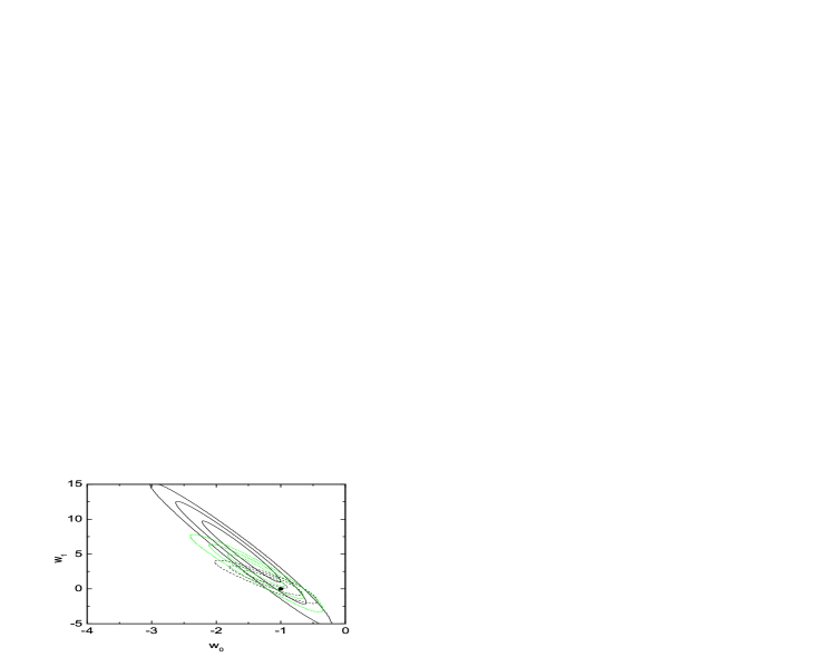
Figure 5: Left panel shows confidence regions derived from 159 SNe Ia. Solid contours refer to the $w(z)=w_{0}+\frac{w_{1}z}{(1+z)^{2}}$ model; green contours, the $w(z)=w_{0}+w_{1}z/(1+z)$ model; dashed contours, the $w_{z}=w_{0}+w_{1}z$ model. The position of a cosmological constant, $(-1,0)$, is marked by a large dot. Right panel shows the transition redshift probability versus. Solid line refers to the $w_{z}=w_{0}+w_{1}z$ model; dashed line, the $w(z)=w_{0}+w_{1}z/(1+z)$ model; dotted line, the $w(z)=w_{0}+w_{1}z/(1+z)^{2}$ model.