Invariant information and complementarity in high-dimensional states

Abstract

Using a generalization of the invariant information introduced by Brukner and Zeilinger [Phys. Rev. Lett. 83, 3354 (1999)] to high-dimensional systems, we introduce a complementarity relation between the local and nonlocal information for $d\times d$ systems under the isolated environment, where $d$ is prime or the power of prime. We also analyze the dynamics of the local information in the decoherence process.

When dealing with classical measurement the Shannon information Shannon:1948 is a natural measure of our ignorance about properties of a system. However, Shannon information is only applicable when measurement reveals a preexisting property. In sharp contrast to classical measurements, a quantum measurement does not reveal a preexisting property. For example, if we want to read out the information encoded in a qubit, we have to project the state of the qubit onto the measurement basis $\left\{{\left|0\right\rangle,\left|1\right\rangle}\right\}$ which will give us a bit value of either 0 or 1. The qubit might be in the eigenstate of the measurement apparatus only in the special case; in general, the value obtained by the measurement has an element of irreducible randomness. Thus we cannot get the value of the bit or even hidden property of the system existing before the measurement is performed. To overcome this difficulty, Brukner and Zeilinger introduced the operationally invariant information Zeilinger:1999 as the measure of local information. The new measure of information is invariant under the transformation from one complete set of complementary variables to another. It is also conserved in time if there is no information exchange between the system and the environment. In this paper, using a generalization of Brukner and Zeilinger’s result to higher dimensional case, we derive a complementarity relation between the local and nonlocal information for $d\times d$ systems.

The new measure is obtained by summing over the measurement outcome of a set of mutually complementary observables (MCO) Ivanovic:1981 ; Wootters:1989 . Before describing the details of our derivations, let us briefly review the definition of MCO. In a $d$-dimensional Hilbert space we call two observables $\mathcal{K}$ and $\mathcal{M}$ mutually complementary if all their respective, complete, orthonormal eigenvectors fulfill

$$\left|{\left\langle{\mathcal{K},k\left|{\mathcal{M},m}\right\rangle}\right.}\right|^{2}=\frac{1}{d}{\kern 1.0pt}{\kern 1.0pt}\;\ \forall k,m=1,\ldots,d.$$ (1)

It is known that if $d$ is prime or the power of prime, the number of MCO is $d+1$ Ivanovic:1981 ; Wootters:1989 ; Bandyopadhyay:2002 ; Bengtsson:2005 ; Romero:2005 ; Wootters:2004 . Consider a measurement of an observable $\mathcal{M}=\sum\nolimits_{j=1}^{d}{a_{j}\Pi_{j}}$. Each outcome $j$ is detected with probability $p_{j}=Tr\rho\Pi_{j}$. According to Ref. Zeilinger:1999 , we define the local invariant information for $d$-level system as

$$I=\mathcal{N}\sum\nolimits_{\alpha=1}^{d+1}{\sum\nolimits_{j=1}^{d}{\left({p_{\alpha j}-\frac{1}{d}}\right)}}^{2},$$ (2)

where $\alpha=1,\ldots,d+1$ and $j=1,\ldots,d$ label complementary observables and their eigenvectors, respectively, and $\mathcal{N}$ is the normalization factors. The derivation of our results use the fact that Ivanovic:1981 ; Wootters:1989

$$Tr\left\{{\Pi_{\alpha j}\Pi_{\beta k}}\right\}=\delta_{\alpha\beta}\delta_{jk}+\frac{1}{p}\left({1-\delta_{\alpha\beta}}\right).$$ (3)

After some algebra, we get

$$I=\frac{d}{d-1}\log_{2}d\left({Tr\rho^{2}-\frac{1}{d}}\right),$$ (4)

where we choose $\log_{2}d$ as the normalization factor to ensure that a $d$-level pure state carries $\log_{2}d$ bits of information. If $d=2^{k}$, $I=\frac{2^{k}k}{2^{k}-1}\left({Tr\rho^{2}-\frac{1}{2^{k}}}\right)$ which corresponds to the local invariant information for composite $k$-qubit systems. The special choice for $k=1,2$ recovers the results obtained in Ref. Zeilinger:1999 .

Next, we want to use this new measure to establish a complementary relation between the local and nonlocal information for $d\times d$ systems. Complementarity is an important concept in quantum theory. Besides the most well-known complementarity principle introduced by Bohr Bohr:1928 , many other kinds of complementarity relation have also been discussed Birula:1975 ; Deutsch:1983 ; Krauss:1987 ; Maassen:1988 . In particular for two-state systems, elegant relations between two complementary observables have been derived Mandel:1991 ; Jaeger:1995 ; Englert:1996 . Additionally, Jakob and Bergou Jakob:2003 have recently derived a complementarity relation for an arbitrary pure state of two qubits. Subsequently, their result was generalized to the multi-qubit systems Tessier:2005 ; Bai:2007 . Recently, Cai et al. Cai:2007 also established an elegant complementarity relation between local and nonlocal information for qubit systems. Below we show that a complementarity relation also holds for $d\times d$ systems.

Now we analyze a two-qutrit system to give an example. Suppose the system initial state is a pure state $\left|\psi\right\rangle_{12}$, and $\rho_{i}$ ($i=1,2$) is the reduced density matrix of each individual qutrit. The total information contained in the $3\times 3$ system is in two forms. One is local form, which is the information content in each individual qutrit. The other is nonlocal form, which is entanglement between the two qutrits. If the $3\times 3$ system is isolated, i.e., it starts with an initial pure and then is subject to unitary transformations only, then the sum of the local and nonlocal information should be conserved. Here, we adopt the operationally invariant information derived above to measure local information. In the case of $3\times 3$ pure state $\left|\psi\right\rangle_{12}$, the local information contained in qutrit 1 and 2 is $I_{1}+I_{2}=\sum\nolimits_{i=1}^{2}{\frac{3}{2}}\log_{2}3\left({Tr\rho_{i}^{2}-\frac{1}{3}}\right)$. If being measured by 2-tangle Coffman:2000 , the pairwise entanglement of the pure state $\left|\psi\right\rangle_{12}$ is $\tau_{12}=C_{12}^{2}=2\left({1-Tr\rho_{i}^{2}}\right)$, where $C_{12}$ is the generalized notion of concurrence for $3\times 3$ pure states Wootters:1998 ; Rungta:2001 . Thus we have the following complementarity relation

$$I_{1}+I_{2}+\left({\frac{3}{2}\log_{2}3}\right)\tau_{12}=2\log_{2}3.$$ (5)

Equation (5) suggests that the nonlocal information has close relation to entanglement, which is a reasonable fact. As every term of $I_{1}$, $I_{2}$ and $\tau_{12}$ is convex, the total expression is. Therefore, $I_{1}+I_{2}+\left({\frac{3}{2}\log_{2}3}\right)\tau_{12}<2\log_{2}3$ for a mixed $3\times 3$ state $\rho_{12}$. This is easy to understand from a physical picture. If the system is not isolated, the $2\log_{2}3$ bit information is not only contained in the system, but also in its correlations with the outside environment. A similar result also holds for $d\times d$ systems if we notice the following fact. For arbitrary $d\times d$ pure state, we have $\tau_{12}=C_{12}^{2}\equiv 2\left({1-Tr\rho_{1}^{2}}\right)=2\left({1-Tr\rho_{2}^{2}}\right)$. Thus, for a $d\times d$ mixed state $\rho_{12}$, the following inequality holds

$$I_{1}+I_{2}+\left({\frac{d}{d-1}\log_{2}d}\right)\tau_{12}\leq 2\log_{2}d.$$ (6)

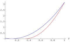
Figure 1: (color online). Plots of $I\left({\rho_{1}}\right)+I\left({\rho_{2}}\right)+\left({\frac{d}{d-1}\log_{2}d}\right)\tau_{12}$ (red line), and $I\left({\rho_{12}}\right)$ (blue line) for $d=3$.

Even though this inequality holds for arbitrary $d\times d$ states, for some special cases we might get a more stringent bound. Consider a class of isotropic mixed states for $d\times d$ systems. These are states invariant under $\rho\rightarrow\int{dU\left({U\otimes U^{\ast}}\right)}\rho\left({U^{{\dagger}}\otimes U^{\ast{\dagger}}}\right)$ and can be expressed as

$$\rho_{iso}\left(F\right)=\frac{1-F}{d^{2}-1}\left({\mathrm{I}-\left|{\Phi^{+}}\right\rangle\left\langle{\Phi^{+}}\right|}\right)+F\left|{\Phi^{+}}\right\rangle\left\langle{\Phi^{+}}\right|,$$ (7)

where $\left|{\Phi^{+}}\right\rangle=\frac{1}{\sqrt{d}}\sum\nolimits_{i=1}^{d}{\left|{ii}\right\rangle}$ and $F\in\left[{0,1}\right]$. For $F\in\left[{0,\frac{1}{d}}\right]$ this state is known to be separable. The tangle for these isotropic states have been obtained in Ref. Rungta:2003 . For $d=3$ the tangle is

$$\tau\left({\rho_{12}}\right)=\left\{{\begin{array}[c]{l}0\ \ \ (F\leq\frac{1}{3})\\ 3\left({F-\frac{1}{3}}\right)^{2}\ \ \ (\frac{1}{3}\leq F\leq 1)\end{array}}\right..$$ (8)

Straightforward calculation shows that the local information for qutrit 1 and qutrit 2 are both 0. Then the value of $I\left({\rho_{1}}\right)+I\left({\rho_{2}}\right)+\left({\frac{3}{2}\log_{2}3}\right)\tau_{12}$ can be calculated using Eq. (8). On the other hand, we consider the local information of the composite 2-qutrit system. Using the formula (4), we obtain $I\left({\rho_{12}}\right)=\frac{9}{4}\left({Tr\rho_{12}^{2}-\frac{1}{9}}\right)=\frac{81F^{2}-18F+1}{32}\log_{2}3$. For a vivid comparison, we plot $I\left({\rho_{1}}\right)+I\left({\rho_{2}}\right)+\left({\frac{3}{2}\log_{2}3}\right)\tau_{12}$ and $I\left({\rho_{12}}\right)$ in Fig. 1. From Fig. 1 we find there always exists the relation $I\left({\rho_{1}}\right)+I\left({\rho_{2}}\right)+\left({\frac{3}{2}\log_{2}3}\right)\tau_{12}<I\left({\rho_{12}}\right)$. Based on this fact, we conjecture that for a general $d\times d$ isotropic mixed state the following inequality is always true

$$I\left({\rho_{1}}\right)+I\left({\rho_{2}}\right)+\left({\frac{d}{d-1}\log_{2}d}\right)\tau_{12}$$

$$\leq\frac{2d^{2}}{d^{2}-1}\log_{2}d\left({Tr\rho^{2}-\frac{1}{d^{2}}}\right).$$ (9)

Note that inequality (9) does not hold for arbitrary $d\times d$ states. It is tempting to define mutual invariant information like the von Neumann entropy. However, this is not reasonable because there does not exist the subadditivity relation for invariant information, i.e., $I\left({\rho_{12}}\right)\leq I\left({\rho_{1}}\right)+I\left({\rho_{2}}\right)$. It only satisfies the additivity relation like $I\left({\rho\otimes\sigma}\right)=I\left(\rho\right)+I\left(\sigma\right)$. In general, we can derive a lower and upper bound of $I\left({\rho_{12}}\right)-I\left({\rho_{1}}\right)-I\left({\rho_{2}}\right)$. First, we can image a $d\times d$ mixed state $\rho_{12}$ is a part of a pure state $\left|\psi\right\rangle_{12R}$, where $R$ denotes a reference system. Usually the reduced density matrix $\rho_{R}$ also lies in a $d\times d$ dimensional Hilbert space. For the composite $d^{2}\times d^{2}$ pure state $\left|\psi\right\rangle_{12R}$ under the cut $12:R$, we have

$$I\left({\rho_{12}}\right)+I\left({\rho_{R}}\right)+\left({\frac{2d^{2}}{d^{2}-1}\log_{2}d}\right)\tau_{12:R}=4\log_{2}d,$$ (10)

where we have used the complementarity relation for pure states. On the other hand, we have

$$I\left({\rho_{1}}\right)+I\left({\rho_{2}}\right)+\left({\frac{d}{d-1}\log_{2}d}\right)\tau_{12}\leq 2\log_{2}d.$$ (11)

Combining Eq. (10) and Eq. (11), we get

$$\begin{array}[c]{l}I\left({\rho_{12}}\right)-I\left({\rho_{1}}\right)-I\left({\rho_{2}}\right)\geq\\ 2\log_{2}d-I\left({\rho_{R}}\right)-{\frac{2d^{2}}{d^{2}-1}}\left({\log_{2}d}\right)\tau_{12:R}+{\frac{d}{d-1}}\left({\log_{2}d}\right)\tau_{12},\\ \end{array}$$ (12)

It is easy to see that the lower bound depends not only on the entanglement of $\rho_{12}$, but also on the entanglement of $\rho_{12}$ with the reference system. It should be noted that this bound can be negative value. For example, consider a seperable two-qubit mixed state ${\rho_{12}}=\frac{5}{12}\left|{00}\right\rangle\left\langle{00}\right|+\frac{4}{12}\left|{01}\right\rangle\left\langle{01}\right|+\frac{2}{12}\left|{10}\right\rangle\left\langle{10}\right|+\frac{1}{12}\left|{11}\right\rangle\left\langle{11}\right|$, one can verify that $I\left({\rho_{12}}\right)-I\left({\rho_{1}}\right)-I\left({\rho_{2}}\right)=-\frac{5}{54}$. The upper bound of $I\left({\rho_{12}}\right)-I\left({\rho_{1}}\right)-I\left({\rho_{2}}\right)$ is easily obtained. We should only consider a $d\times d$ maximally entangled pure state $\left|\psi\right\rangle_{12}=\frac{1}{\sqrt{d}}\sum\nolimits_{j=1}^{d}{\left|{ii}\right\rangle}$. The local information $I\left({\rho_{1}}\right)$ and $I\left({\rho_{2}}\right)$ for this special pure state are both 0, while $I\left({\rho_{12}}\right)$ reaches a maximum value $2\log_{2}d$. Therefore we have $I\left({\rho_{12}}\right)-I\left({\rho_{1}}\right)-I\left({\rho_{2}}\right)\leq 2\log_{2}d$. The above analysis suggests that we cannot treat invariant information in the same way as the von Neumann entropy; sometimes we might resort to the von Neumann entropy to gain a more comprehensive insight into the quantum information. Invariant information provides a complement of the von Neumann entropy in the description of quantum information, but cannot substitute the role of the von Neumann entropy. Perhaps a deeper investigation of invariant information is desired.

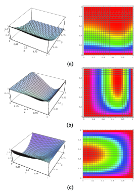
Figure 2: (color online). The plots of the local information for the state $\left|\psi\right\rangle_{12}=a\left|{00}\right\rangle+\sqrt{1-a^{2}}\left|{11}\right\rangle$ in the three decoherence processes. The right pannels are plotted in the density form of the left ones.

So far, we only consider the systems in the isolated environment. One can easily visualize that the local information will decrease in open systems. In order to gain more insight into the above question, we analyze the behaviour of simple two-qubit entangled states under decoherence. We choose the depolarization, dephasing, and dissipation channel as our toy model for decoherence.

Consider the two-qubit state $\left|\psi\right\rangle_{12}=a\left|{00}\right\rangle+\sqrt{1-a^{2}}\left|{11}\right\rangle$ where $a$ is real number with $0\leq a\leq 1$. We define $p$ as the degree of decoherence of an individual qubit, which lies between 0 and 1. Here the value 0 means no decoherence, and 1 means complete decoherence. The depolarization process with a decoherence degree $p$ is described by

$$\left|i\right\rangle\left\langle j\right|\rightarrow\left({1-p}\right)\left|i\right\rangle\left\langle j\right|+p\delta_{ij}\frac{I}{2}.$$ (13)

The dephasing process is represented by

$$\left|i\right\rangle\left\langle j\right|\rightarrow\left({1-p}\right)\left|i\right\rangle\left\langle j\right|+p\delta_{ij}\left|i\right\rangle\left\langle j\right|.$$ (14)

The dissipation is an energy-lossing process, and thus changes the state to a specific state. We choose $\left|0\right\rangle$ as the ground state. Then the dissipation process is described by

$$\begin{array}[c]{l}\left|i\right\rangle\left\langle i\right|\rightarrow\left({1-p}\right)\left|i\right\rangle\left\langle i\right|+p\left|0\right\rangle\left\langle 0\right|,\\ \left|i\right\rangle\left\langle j\right|\rightarrow\left({1-p}\right)^{\frac{1}{2}}\left|i\right\rangle\left\langle j\right|,\;\;\mbox{where}\;i\neq j.\end{array}$$ (15)

After the action of the depolarization channel, the local information of the 2-qubit system is given by

$$\begin{array}[]{l}I=\frac{2}{3}\left({4Tr\rho^{2}-1}\right)\\ =\frac{2}{3}\left\{{4\left[{a^{2}\left({1-a^{2}}\right)}\right.}\right.\left({2p^{4}-8p^{3}+10p^{2}-4p}\right)\\ \left.{\left.{+\frac{1}{4}p^{4}-p^{3}+2p^{2}-2p+1}\right]-1}\right\}\\ \end{array}.$$ (16)

We plot Eq. (16) in Fig. 2(a), and the local information under the dephasing and dissipation processes are plotted in Fig. 2(b) and (c), respectively. It shows in Fig. 2 that the minimum value of the local information of the 2-qubit systems is 0 for the depolarization channel while it is always a positive value for the other two channels. The main reason is due to the fact that the depolarization channel will transform the initial state into a totally mixed state after infinite time, while the local information for maximally mixed state is 0.

Before concluding we would like to stress that our complementarity relation is based on invariant information. This perspective is different from the methods used in Refs. Oppenheim:2002 ; Horodecki:2003 ; Horodecki:2005 ; Horodecki1:2005 , where the authors utilized the von Neumann entropy to investigate the complementarity between local and nonlocal information. The distinct advantage by using invariant information is based on the following facts. The first is that invariant information always implies additivity, which is a desired property to establish complementarity relations. The second is that invariant information can be directly related to the tangle of $d\times d$ pure states. The third nice feature of the invariant information is that its definition is operational. It is obtained by synthesizing the errors of a specially chosen set of measurements performed on the system. Thus we might get a different insight into the complementarity relation between the local and nonlocal information.

Summarizing, we have generalized the invariant information introduced by Brukner and Zeilinger. For $d\times d$ mixed states (where $d$ is prime or the power of prime), using the invariant information, we establish a complementarity relation between the local and nonlocal information under the isolated environment. Furthermore, we show that the nonlocal information has a direct relation with the entanglement of the system. Some differences between the invariant information and von Neumann entropy are also discussed. We also investigate the dynamics of the local information in the open systems through a simple example.

W.S. thanks Jian-Ming Cai for valuable discussions. This work was supported by the NNSF of China, the CAS, and the National Fundamental Research Program (under Grant No. 2006CB921900).

References

- (1) C. E. Shannon, Bell Syst. Tech. J. 27, 379 (1948).
- (2) C. Brukner and A. Zeilinger, Phys. Rev. Lett. 83, 3354 (1999).
- (3) I. D. Ivanovic, J. Phys. A 14, 3241 (1981).
- (4) W. K. Wootters and B. D. Fields, Ann. Phys. (N.Y.) 191, 363 (1989).
- (5) S. Bandyopadhyay, P. O. Boykin, V. Roychowdhury, and F. Vatan, Algorithmica 34, 512 (2002).
- (6) I. Bengtsson and A. Ericsson, Open Syst. Inf. Dyn. 12, 107 (2005).
- (7) J. L. Romero, G. Bjork, A. B. Klimov, and L. L. Sanchez-Soto, Phys. Rev. A 72, 062310 (2005).
- (8) W. K. Wootters, e-print quant-ph/0406032.
- (9) N. Bohr, Nature (London) 121, 580 (1928); N. Bohr, Phys. Rev. 48, 696 (1935).
- (10) I. Bialynicki-Birula and J. Mycielski, Commun. Math. Phys. 44, 129 (1975).
- (11) D. Deutsch, Phys. Rev. Lett. 50, 631 (1983).
- (12) K. Krauss, Phys. Rev. D 35, 3070 (1987).
- (13) H. Maassen and J. B. M. Uffink, Phys. Rev. Lett. 60, 1103 (1988).
- (14) L. Mandel, Opt. Lett. 16, 1882 (1991).
- (15) G. Jaeger, A. Shimony, and L. Vaidman, Phys. Rev. A 51, 54 (1995).
- (16) B.-G. Englert, Phys. Rev. Lett. 77, 2154 (1996).
- (17) M. Jakob, J. A. Bergou, quant-ph/0302075.
- (18) T. E. Tessier, Found. Phys. Lett. 18, 107 (2005).
- (19) Y.-K. Bai, D. Yang, Z. D. Wang, quant-ph/0703098.
- (20) J.-M. Cai, Z.-W. Zhou, X.-X. Zhou, and G.-C. Guo, Phys. Rev. A 74, 042338 (2006); J.-M. Cai, Z.-W. Zhou, G.-C. Guo, Phys. Lett. A 363, 392 (2007).
- (21) V. Coffman, J. Kundu, and W. K. Wootters, Phys. Rev. A 61, 052306 (2000).
- (22) W. K. Wootters, Phys. Rev. Lett. 80, 2245 (1998).
- (23) P. Rungta, V. Buzek, C.M. Caves, M. Hillery, and G.J. Milburn, Phys. Rev. A 64, 042315 (2001).
- (24) P. Rungta and C. M. Caves, Phys. Rev. A 67, 012307 (2003).
- (25) J. Oppenheim, M. Horodecki, P. Horodecki, and R. Horodecki, Phys. Rev. Lett. 89, 180402 (2002).
- (26) M. Horodecki, K. Horodecki, P. Horodecki, R. Horodecki, J. Oppenheim, A. Sen(De), and U. Sen, Phys. Rev. Lett. 90, 100402 (2003).
- (27) M. Horodecki, P. Horodecki, R. Horodecki, J. Oppenheim, A. Sen(De), U. Sen, and B. Synak-Radtke, Phys. Rev. A 71, 062307 (2005).
- (28) M. Horodecki, J. Oppenheim, and A. Winter, Nature (London) 436, 673 (2005).