Best network chirplet-chain: Near-optimal coherent detection of unmodeled gravitation wave chirps with a network of detectors

Abstract

The searches of impulsive gravitational waves (GW) in the data of the ground-based interferometers focus essentially on two types of waveforms: short unmodeled bursts from supernova core collapses and frequency modulated signals (or chirps) from inspiralling compact binaries. There is room for other types of searches based on different models. Our objective is to fill this gap. More specifically, we are interested in GW chirps “in general”, i.e., with an arbitrary phase/frequency vs. time evolution. These unmodeled GW chirps may be considered as the generic signature of orbiting or spinning sources. We expect the quasi-periodic nature of the waveform to be preserved independently of the physics which governs the source motion. Several methods have been introduced to address the detection of unmodeled chirps using the data of a single detector. Those include the best chirplet chain (BCC) algorithm introduced by the authors. In the next years, several detectors will be in operation. Improvements can be expected from the joint observation of a GW by multiple detectors and the coherent analysis of their data namely, a larger sight horizon and the more accurate estimation of the source location and the wave polarization angles. Here, we present an extension of the BCC search to the multiple detector case. This work is based on the coherent analysis scheme proposed in the detection of inspiralling binary chirps. We revisit the derivation of the optimal statistic with a new formalism which allows the adaptation to the detection of unmodeled chirps. The method amounts to searching for salient paths in the combined time-frequency representation of two synthetic streams. The latter are time-series which combine the data from each detector linearly in such a way that all the GW signatures received are added constructively. We give a proof of principle for the full sky blind search in a simplified situation which shows that the joint estimation of the source sky location and chirp frequency is possible.

I Summary

A large effort is underway to analyze the scientific data acquired jointly by the long-baseline interferometric gravitational wave (GW) detectors GEO 600, LIGO, TAMA and Virgo det . In this paper, we contribute to the methodologies employed for this analysis, and in particular for the detection of impulsive GW signals.

The current GW data analysis effort is targeted on two types of impulsive GWs. A first target is poorly known short bursts of GWs with a duration in the hundredth of a millisecond range. The astrophysically known sources of such GW bursts are supernovae core collapses (or other similar cataclysmic phenomenon). The second target is frequency modulated signals or chirps radiated by inspiralling binaries of compact objects (either neutron stars (NS) or black holes (BH)). These chirp waveforms are well modeled and expected to last for few seconds to few minutes in the detector bandwidth. Our objective is to enlarge the signal range of impulsive GWs under consideration and to fill this gap between these two types. More specifically, we are interested in the detection of unmodeled GW chirps which last from few tens of milliseconds to few seconds in the detector bandwidth. We shall detail in the next section the astrophysical motivation for considering this kind of GWs.

Simultaneous observation and analysis of the jointly observed data from different GW detectors has definite obvious benefits. First and foremost, a GW detection can get confirmed or vetoed out with such a joint observation. Further, the detector response depends on the position and orientation of the source and polarization of the wave. For this reason, the joint observation by multiple detectors gives access to physical parameters such as source location and polarization. The use of multiple detectors also allows to enlarge the observational horizon and sky coverage.

Till date, several methods have been proposed and implemented to detect unmodeled GW chirps using a single detector which include the signal track search (STS) Anderson and Balasubramanian (1999), the chirplet track search Candès et al. (2007) and the best chirplet chain (BCC) search proposed by the authors Chassande-Mottin and Pai (2006). However, none of the above addresses the multiple detector case. This requires the designing of specific algorithms which are able to combine the information received by the different detectors.

In practice, there are two approaches adopted to carry out network analysis from many detectors, coincidence and coherent approach. In coincidence approach, the data from each detector is processed independently and only coincident trigger events (in the arrival time and the parameter values) are retained and compared. On the other hand, in the coherent approach, the network as a whole is treated as a single “sensor”: the data from various detectors is analyzed jointly and combined into a single network statistic which is tested for detection. In the literature, it has been shown that the coherent approach performs better than the coincidence approach for GW short bursts Arnaud et al. (2003) as well as GW chirps from coalescing binaries Mukhopadhyay et al. (2006). Indeed, the signal phase information is preserved with the coherent approach, whereas it is not with the coincidence approach which therefore leads to some information loss. Thus, we wish to follow the coherent approach for our analysis.

Another reason for this choice is that the coincidence method is not adequate for unmodeled chirps. A large number of parameters (in the same order as the number of signal samples) is needed to characterize their frequency evolution. A coincident detection occurs when the parameter estimates obtained from the analysis of the individual detector data match. Because of the noise fluctuation, the occurrence of such a coincidence is very unlikely when the number of parameters is large, unless the incoming GW has very large amplitude. In this article, we therefore adopt the coherent method and propose the coherent extension of the BCC algorithm.

Coherent schemes have been already developed for the detection of inspiralling binary chirps Pai et al. (2001); Finn (2001). Here, we revisit the work presented in Pai et al. (2001) with a new formalism. Comments in footnotes link the results presented here with the ones of Pai et al. (2001). We show that the new formalism presented here helps to understand the geometry of the problem and it is simple to establish connections with earlier works.

The outline of the paper goes as follows. In Sec. II, we present and motivate our model of an arbitrary GW chirp. In Sec. III, we describe the response of the detector network to an incoming GW chirp. Further, we show that the linear component of the signal model (parameters acting as scaling factors and phase shifts, so called extrinsic parameters) can be factorized. This factorization evidences that the signal space can be represented as the direct product of two two-dimensional spaces i.e., the GW polarization plane and the chirp plane. This representation forms the backbone of the coherent detection scheme that follows in the subsequent section.

In Sec. IV, based on a detailed geometrical argument, we show that the above signal representation manifests the possible degeneracy of the response. This degeneracy has been already noticed and studied at length in the context of burst detection Klimenko et al. (2005); Mohanty et al. (2006); Rakhmanov (2006). We investigate this question in the specific context of chirps and obtain similar results as were presented earlier in the literature.

In Sec. V, we obtain the expression of the network statistic. Following the principles of the generalized likelihood ratio test (GLRT), the statistic is obtained by maximizing the network likelihood ratio over the set of unknown parameters. We perform this maximization in two steps. We first treat the linear part of the parameterization and show that such a maximization is nothing but a least square problem over the extrinsic parameters. The solution is obtained by projecting the data onto the signal space. We further study the effect of the response degeneracy on the resulting parameter estimates.

The projection onto the signal space is a combined projection onto the GW polarization and chirp planes. The projection onto the first plane generates two synthetic streams which can be viewed as the output of “virtual detectors”. The network statistic maximized over the extrinsic parameters can be conveniently expressed in terms of the processing of those streams. In practice, the synthetic streams linearly combine the data from each detector in such a way that the GW signature received by each detector is added constructively. With this rephrasing, the source location angles can be searched over efficiently.

Along with the projection onto the GW polarization plane, we also examine the projection onto its complement. While synthetic streams concentrate the GW contents, the so called null streams produced this way combines the data such that the GW signal is canceled out. The null streams are useful to veto false triggers due to instrumental artifacts (which don’t have this cancellation property). The null streams we obtained here are identical to the ones presented earlier in GW burst literature Guersel and Tinto (1990); Wen and Schutz (2005); Chatterji et al. (2006).

In Sec. VI, we perform the second and final step of the maximization of the network statistic over the chirp phase function. This step is the difficult part of the problem. For the one detector case, we have proposed an efficient method, the BCC algorithm which addresses this question. We show that this scheme can be adapted to the multiple detector case in a straightforward manner, hence refer to this as Best Network CC (BNCC).

Finally, Sec. VII presents a proof of principle of the proposed method with a full-sky blind search in a simplified situation.

II Generic GW chirps

II.1 Motivation

Known observable GW sources e.g., stellar binary systems, accreting stellar systems or rotating stars, commonly involve either orbiting or spinning objects. It is not unreasonable to assume that the similar holds true even for the unknown sources.

The GW emission is essentially powered by the source dynamics which thus determines the shape of the emitted waveform. Under linearized gravity and slow motion (i.e., the characteristic velocity is smaller than the speed of light) approximation, the quadrupôle formula Flanagan and Hughes (2005) predicts that the amplitude of emitted GW is proportional to the second derivative of the quadrupôle moment of the physical system. When the dominant part of the bulk motion follows an orbital/rotational motion, the quadrupôle moment varies quasi-periodically, and so is the GW.

The more the information we have about the GW signal, the easier/better is the detection of its signature in the observations. Ideally, this requires precise knowledge of the waveform, and consequently requires precise knowledge of the dynamics. This is not always possible. In general, predicting the dynamics of GW sources in the nearly relativistic regime requires a large amount of effort. This task may get further complicated if the underlying source model involves magnetic couplings, mass accretion, density-pressure-entropy gradients, anisotropic angular momentum distribution.

Here, we are interested in GW sources where the motion is orbital/rotational but the astrophysical dynamics is (totally or partially) unknown. While our primary target is the unforeseen sources (this is why we remain intentionally vague on the exact nature of the sources), several identified candidates enter this category because their dynamics is still not fully characterized. These include (see Chassande-Mottin and Pai (2006) for more details and references) binary mergers, quasi normal modes from young hot rotating NS, spinning BH accreting from an orbiting disk. As motivated before, following the argument of quadrupôle approximation, the GW signature for such sources is not completely undetermined: it is expected to be quasi-periodic, possibly frequency modulated GW ; in brief, it is a GW chirp. This is the basic motivation for introducing a generic GW chirp model, as described in the next section.

II.2 Generic GW chirp model

In this section, we describe the salient features of the generic GW chirp model used in this paper. We motivate the nature of GW polarization, the regularity of its phase and frequency evolution.

II.2.1 Relation between the polarizations

The GW tensor (in transverse traceless (TT) gauge), associated to the GW emitted from slow-motion, weak gravity sources are mostly due to variations of the mass moments (in contrast to current moments) and can be expanded in terms of mass multipole moments as Thorne (1980)

$$h^{TT}(t)\propto\sum_{l=2}^{\infty}\sum_{m=-l}^{l}(\nabla\nabla Y^{lm})^{\rm STF}\frac{d^{l}}{{dt}^{l}}I^{lm}(t-r/c).$$ (1)

Here, STF means “symmetric transverse-tracefree”, $Y^{lm}$ are the spherical harmonics, and $I^{lm}$ are the mass multipole moments.

We consider here isolated astrophysical systems with anisotropic mass distributions (e.g., binaries, accreting systems, bar/fragmentation instabilities) orbiting/rotating about a well-defined axis. It can be shown that these systems emit GW predominantly in the $l=|m|=2$ mode. Contributions from any other mass moments are negligibly small . The pure-spin tensor harmonic $(\nabla\nabla Y^{lm})^{\rm STF}$ term provides the GW polarization. For $l=|m|=2$ mode, we have

$$(\nabla\nabla Y^{22})^{\rm STF}\propto(1+\cos^{2}\epsilon)e_{+}+2i\cos\epsilon\;e_{\times}.$$ (2)

The tensors $e_{+}$ and $e_{\times}$ form a pair of independent and linear-polarization GW tensors ($e_{\times}$ is rotated by and angle $\pi/4$ with respect to $e_{+}$). The orbital inclination angle $\epsilon$ is the angle between the line of sight to the source (in Earth’s frame) and the angular momentum vector (or the rotation axis) of the physical system, see Fig. 1 (a). This shows that the emitted GW in the considered case carries both GW polarizations.

The GW tensor is fully described as $h^{TT}(t)=h_{+}(t)e_{+}+h_{\times}(t)e_{\times}$. The phase shift between the two polarizations $h_{+}$ and $h_{\times}$ arises from the $I^{lm}$ term which is proportional to the moment of inertia tensor for $l=|m|=2$. The quadratic nature of the moment of inertia tensor introduces a phase shift of $\pi/2$ between the two polarizations $h_{+}$ and $h_{\times}$. This leads to the chirp model below

$$h_{+}(t) = A\frac{1+\cos^{2}\epsilon}{2}\>\cos(\varphi(t-t_{0})+\phi_{0})\,,$$ (3a)

$$h_{\times}(t) = A\cos\epsilon\>\sin(\varphi(t-t_{0})+\phi_{0}),$$ (3b)

with $t_{0}\leq t<t_{0}+T$ and $h_{+,\times}(t)=0$ outside this interval. The phase $\phi_{0}$ is the signal phase at $t=t_{0}$.

Here, we assume the GW amplitude $A$ to be constant. This is clearly an over-simplified case since we indeed expect an amplitude modulation for real GW sources. However we wish here to keep the model simple in order to focus the discussion on the aspects related to the coherent analysis of data from multiple detectors. We postpone the study of amplitude modulated GWs to future work.

The chirp model described in Eq. (3) clearly depends upon several unknown parameters (which need to be estimated from the data) which include the amplitude $A$, the initial phase $\phi_{0}$, the arrival time $t_{0}$ of the chirp and the inclination angle $\epsilon$. As no precise assumption on the exact nature and dynamics of the GW source is made, we consider the phase evolution function $\varphi(\cdot)$ to be an unknown parameter of the model (3) as well. Clearly, it is a more complicated parameter than the others which are simply scalars. Just like any scalar parameter can be constrained to a range of values (e.g., $A>0$), the phase function $\varphi(\cdot)$ has to satisfy conditions to be physically realistic which we describe in the next section.

II.2.2 Smoothness of the phase evolution

As explained above, the chirp phase is directly related to the orbital phase of the source. The regularity of the orbital phase can be constrained by the physical arguments: the orbital phase and its derivatives are continuous. The same applies to the chirp phase and derivatives.

The detectors operate in a frequency window limited in the range from few tenths of Hz to a kHz and they are essentially blind outside. This restricts our interest to sources emitting in this frequency range, which results in lower and upper limits on the chirp frequency $\nu(t)\equiv(2\pi)^{-1}d\varphi/dt$ and thus on the variations of the phase.

In addition, the variation of the frequency (the chirping rate) can be connected to the rate at which the source loses its energy. For isolated systems, this is clearly bounded. This argument motivates the following bounds on the higher-order derivatives of the phase:

$$\left|\frac{d\nu}{dt}\right| \leq F^{\prime}, \left|\frac{d^{2}\nu}{dt^{2}}\right| \leq F^{\prime\prime}.$$ (4)

In this sense, Eq.(4) determines and strengthens the smoothness of the phase/frequency evolution. This is the reason why we coined the term “smooth GW chirp” in Chassande-Mottin and Pai (2006). The choice of the allowed upper bounds $F^{\prime}$ and $F^{\prime\prime}$ may be based on general astrophysical arguments on the GW source of interest.

III Response of a network of detectors to an incoming GW

After describing the chirp model in the previous section, in this section we derive the response of a network of interferometric ground based detectors with arbitrary locations and orientations to an incoming GW chirp. The first step towards this is to identify the coordinate frames.

III.1 Coordinate frames

We follow the conventions of Pai et al. (2001) and introduce three coordinate frames, namely, the wave frame, the Earth frame and the detector frame as given below, see Fig. 1.

• the wave frame $\mathbf{x}_{w}\equiv(x_{w},y_{w},z_{w})$ is the frame associated to the incoming GW with positive $z_{w}$-direction along the incoming direction and $x_{w}-y_{w}$ plane corresponds to the plane of the polarization of the wave.

• the Earth frame $\mathbf{x}_{E}\equiv(x_{E},y_{E},z_{E})$ is the frame attached to the center of the Earth. The $x_{E}$ axis is radially pointing outwards from the Earth’s center and the equatorial point that lies on the meridian passing through Greenwich, England. The $z_{E}$ axis points radially outwards from the center of Earth to the North pole. The $y_{E}$ axis is chosen to form a right-handed coordinate system with the $x_{E}$ and $z_{E}$ axes.

• the detector frame $\mathbf{x}_{d}\equiv(x_{d},y_{d},z_{d})$ is the frame attached to the individual detector. The $(x_{d}-y_{d})$ plane contains the detector arms and is assumed to be tangent to the surface of the Earth. The $x_{d}$ axis bisects the angle between the detector’s arms. The $z_{d}$ axis points towards the local zenith. The direction of the $y_{d}$ axis is chosen so that we get a right-handed coordinate system.

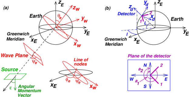
Figure 1: Color online — Coordinate transformations. (a) ${\cal O}(\phi_{e},\theta_{e},\psi_{e})$: Earth frame $\mathbf{x}_{E}:(x_{E},y_{E},z_{E})\rightarrow$ wave frame $\mathbf{x}_{w}:(x_{w},y_{w},z_{w})$, (b) ${\cal O}(\alpha,\beta,\gamma)$: Earth frame $\mathbf{x}_{E}:(x_{E},y_{E},z_{E})\rightarrow$ detector frame: $\mathbf{x}_{d}:(x_{d},y_{d},z_{d})$. The latitude $l$ and longitude $L$ of the detector are related to the Euler angles by Eqs. (8) and (9).

Table 1: Location and orientation informations of the Earth-based interferometric GW detectors. The location of the corner station (vertex) of each detector is given in terms of the latitude and longitude. The orientation of an arm is given by the angle through which one must rotate it clockwise (while viewing from top) to point the local North. The corresponding detector Euler angles $(\alpha,\beta,\gamma)$ are listed.

Detector	Vertex	Vertex	Arm 1	Arm 2	$\alpha$	$\beta$	$\gamma$
	latitude (N)	longitude (E)	$a_{1}$	$a_{2}$
TAMA-300 (T)	$35^{\circ}40^{\prime}35.6^{\prime\prime}$	$139^{\circ}32^{\prime}9.8^{\prime\prime}$	$90.0^{\circ}$	$180.0^{\circ}$	$229.54^{\circ}$	$54.32^{\circ}$	$225^{\circ}$
GEO-600 (G)	$52^{\circ}14^{\prime}42.528^{\prime\prime}$	$9^{\circ}48^{\prime}25.894^{\prime\prime}$	$25^{\circ}56^{\prime}35^{\prime\prime}$	$291^{\circ}36^{\prime}42^{\prime\prime}$	$99.81^{\circ}$	$37.75^{\circ}$	$68.778^{\circ}$
VIRGO (V)	$43^{\circ}37^{\prime}53.0921^{\prime\prime}$	$10^{\circ}30^{\prime}16.1878^{\prime\prime}$	$341^{\circ}25^{\prime}57.2^{\prime\prime}$	$70^{\circ}34^{\prime}2.8^{\prime\prime}$	$100.5^{\circ}$	$46.37^{\circ}$	$116.0^{\circ}$
LIGO Hanford (LH)	$46^{\circ}27^{\prime}18.528^{\prime\prime}$	$-119^{\circ}25^{\prime}27.5657^{\prime\prime}$	$35.9994^{\circ}$	$125.9994^{\circ}$	$-29.41^{\circ}$	$43.55^{\circ}$	$171.0^{\circ}$
LIGO Livingstone (LL)	$30^{\circ}33^{\prime}46.4196^{\prime\prime}$	$-90^{\circ}46^{\prime}27.2654^{\prime\prime}$	$107.7165^{\circ}$	$197.7165^{\circ}$	$-0.77^{\circ}$	$59.44^{\circ}$	$242.72^{\circ}$

A rotation transformation between the coordinate systems about the origin is specified by the rotation operator ${\cal O}$ which is characterized by these three Euler angles. We define these angles using the “$x$-convention” (also known as $z-x-z$ convention) Goldstein (1980).

Let $(\phi_{e},\theta_{e},\psi_{e})$ and $(\alpha,\beta,\gamma)$ be Euler angles of the rotation operator relating pairs of the above coordinate systems as follows

$$\mathbf{x}_{w} = {\cal O}(\phi_{e},\theta_{e},\psi_{e})\mathbf{x}_{E},$$ (5)

$$\mathbf{x}_{d} = {\cal O}(\alpha,\beta,\gamma)\mathbf{x}_{E}.$$ (6)

All the angles in the Eqs. (5) and (6) are related to physical/geometrical quantities described in Fig. 1. More specifically, we have

$$\phi_{e} =\phi-\pi/2, \theta_{e} =\pi-\theta, \psi_{e} =\psi,$$ (7)

where $\phi$ and $\theta$ are the spherical polar coordinates of the source in the Earth’s frame and the angle $\psi$ is the so-called polarization-ellipse angle which gives the orientation of the source plane. Throughout the paper, we shall use $\theta$ and $\phi$ to indicate the source location.

The detector Euler angles $(\alpha,\beta,\gamma)$ are directly related to the location and orientation of the detector as follows:

$$\alpha =L+\pi/2,$$ (8)

$$\beta =\pi/2-l,$$ (9)

$$\gamma =\frac{a_{1}+a_{2}}{2}+\frac{3\pi}{2} \text{if $|a_{1}-a_{2}|>\pi$},$$ (10)

$$=\frac{a_{1}+a_{2}}{2}+\frac{\pi}{2} \text{if $|a_{1}-a_{2}|\leq\pi$},$$ (11)

where $l$ and $L$ are the latitude and longitude of the corner station. The angles $a_{1}$ and $a_{2}$ describe the orientation of the first and second arm respectively. It is the angle through which one must rotate the arm clockwise (while viewing from top) to point the local North. In Table 1, we tabulate the currently running interferometric detectors along with their Euler angles.

Combining Eqs. (5) and (6), we obtain the coordinate transformation from the wave frame to the detector frame as follows

$$\mathbf{x}_{s}={\cal O}(\phi^{\prime}_{e},\theta^{\prime}_{e},\psi^{\prime}_{e})\mathbf{x}_{d}\,,$$ (12)

where ${\cal O}(\phi^{\prime}_{e},\theta^{\prime}_{e},\psi^{\prime}_{e})\equiv{\cal O}(\phi_{e},\theta_{e},\psi_{e}){\cal O}^{-1}(\alpha,\beta,\gamma)$.

III.2 Network response

An interferometric response to the incident GW is obtained by contracting a GW tensor with the detector tensor [see Appendix B], which can be re-expressed as a linear combination of the two polarizations $h_{+}$ and $h_{\times}$ i.e.

$$s = f_{+}h_{+}+f_{\times}h_{\times}$$ (13)

$$\equiv \Re[f^{*}h],$$

and the linear coefficients $f_{+}(\phi^{\prime}_{e},\theta^{\prime}_{e},\psi^{\prime}_{e})$ and $f_{\times}(\phi^{\prime}_{e},\theta^{\prime}_{e},\psi^{\prime}_{e})$, commonly termed as the detector antenna pattern functions, represent the detector’s directional response to the $+$ and $\times$ polarizations respectively. For the compact expression provided by Eq. (13), we have defined the complex GW signal to be $h=h_{+}+ih_{\times}$ and the complex antenna pattern function to be $f=f_{+}+if_{\times}$.

The detector response $s$ and the incident GW signal $h$ are both times series. In a network where the various detectors are located at different locations on the Earth, for example the LIGO-Virgo network, the GW will arrive at the detector sites at different time instances. However, all the measurements at the various detectors need to be carried out with a reference time. Here, just for our convenience, we choose the observer attached to the Earth’s center as a reference and the time measured according to this observer is treated as a reference. Any other reference would be equally acceptable.

Assuming that the detector response is labeled with this time reference (a single reference time for all detectors in a detector network), we have

$$s(t)=\Re[f^{*}h(t-\tau(\phi,\theta))],$$ (14)

where $\tau(\phi,\theta)=(\mathbf{r}_{d}-\mathbf{r}_{E})\cdot\mathbf{w}(\phi,\theta)/c$ denotes the difference in the arrival times of the GW (propagating with the unit wave vector $\mathbf{w}$) at the detector and at the center of the Earth located at $\mathbf{r}_{d}$ and $\mathbf{r}_{E}$, respectively. Note that this value can be positive or negative depending on the source location.

III.3 Vector formalism

In the following, we distinguish scalars by using roman letters, vectors are denoted by small bold letters, and matrices by bold capitals. We denote the $k$-th element of vector $\mathbf{a}$ by $a[k]$ and correspondingly, the element of matrix $\mathbf{A}$ at row $k$ and column $l$ by $A[k,l]$. The matrices $\mathbf{A}^{T}$ and $\mathbf{A}^{H}\equiv(\mathbf{A}^{T})^{*}$ designate the real and hermitian transposes of $\mathbf{A}$ respectively.

We consider now a GW detector network with $d$ interferometers. Each detector and its associated quantities are labeled with an index $j=1,\dots,d$ which we also use as a subscript if required. We assume that the output response of each detector is sampled at the Nyquist rate $\nu_{s}\equiv 1/t_{s}$ where $t_{s}$ is the sampling interval. We then divide the data in blocks of $N$ consecutive samples. In this set-up, the detector as well as the network response is then defined by forming vectors with these blocks of data.

Let us consider a given GW chirp source at sky location $(\phi,\theta)$. Let the response of the $j$-th detector be $\mathbf{s}_{j}$ with entry $s_{j}[k]=s_{j}(t_{k}+\tau_{j}(\phi,\theta))$, where $t_{k}=t_{0}+kt_{s}$, $k=0,\ldots,N-1$, and $t_{0}$ is the reference time i.e. the time of arrival of GW at the center of the Earth. Note that, with the above definition, we compensate for the time delay $\tau_{j}(\phi,\theta)$ between the detector $j$ and the Earth’s center. Thus, in this set-up, the GW signal starts and ends in the same rows in the data vectors $\mathbf{s}_{j}$ of all the detectors.

For compactness, we stack the data from all the detectors in the network into a single vector $\mathbf{s}$ of size $Nd\times 1$, such that $\mathbf{s}^{T}=[\mathbf{s}_{1}^{T}\mathbf{s}_{2}^{T}\ldots\mathbf{s}_{d}^{T}]$ forms the network response. In this convention, the network response can be expressed compactly as the Kronecker product (see Appendix A for the definition) of the network complex beam pattern vector $\mathbf{f}=\{f_{j},j=1\ldots d\}\in\mathbb{C}^{d\times 1}$ and the complex GW vector $\mathbf{h}=\{h(t_{k}),t_{k}=t_{0}+t_{s}k\mathrm{~{}with~{}}k=0\ldots N-1\}\in\mathbb{C}^{N\times 1}$ viz.,

$$\mathbf{s}=\Re[\mathbf{f}^{*}\otimes\mathbf{h}].$$ (15)

The above expression is general enough to hold true for any type of incoming GW signal. The Kronecker product in this expression is the direct manifestation of the fact that the detector response is nothing but the tensor product between the detector and the wave tensors.

III.4 GW chirp as a linear model of the extrinsic parameters

In previous section, we have obtained the network response to any type of incoming GW with two polarizations. In what follows, we wish to investigate how this response manifests in case of a specific type of GW, namely GW chirp described in Eq. (3). We also want to understand how various parameters explicitly appear in the network response.

It is insightful to distinguish the signal parameters based on their effect on the signal model. The parameters are separated into two distinct types traditionally referred to as the “intrinsic” and “extrinsic” parameters. The extrinsic parameters are those that introduce scaling factors or phase shifts but do not affect the shape of the signal model. Instead, intrinsic parameters significantly alter the shape of the signal and hence the underlying geometry.

The network response $\mathbf{s}$ mingles these two types of parameters. Our work is considerably simplified if we can “factorize” the extrinsic parameters from the rest. For the chirp model described in Eq. (3), we count four extrinsic parameters, namely $\{A,\phi_{0},\epsilon,\psi_{e}\}$ and perform this factorization in two steps.

III.4.1 Extended antenna pattern includes the inclination angle

We absorb the inclination angle $\epsilon$ into the antenna pattern functions and rewrite the network signal as

$$\mathbf{s}=\Re[\mathbf{\tilde{f}}^{*}\otimes\mathbf{\tilde{h}}],$$ (16)

where $\mathbf{\tilde{h}}\equiv a\mathbf{e}$ is the GW vector. It only depends on the complex amplitude $a=A\exp i\phi_{0}$ and on the phase vector $\mathbf{e}=\{\exp(i\varphi[k]),\text{ with }\varphi[k]\equiv\varphi(kt_{s}),k=0\ldots N-1\}$.

The extended antenna pattern $\mathbf{\tilde{f}}$ incorporates the inclination angle $\epsilon$ as follows

$$\mathbf{\tilde{f}}=\frac{1+\cos^{2}\epsilon}{2}~{}\mathbf{f}_{+}+i\cos\epsilon~{}\mathbf{f}_{\times}\,.$$ (17)

III.4.2 Gel’fand functions factorize the polarization angles from source location angles

The second step is to separate the dependency of $\mathbf{\tilde{f}}$ on the polarization angles $\{\psi,\epsilon\}$ from the source location angle and the detector orientation angles. The earlier work Pai et al. (2001) shows that the Gel’fand functions (which are representation of the rotation group $SO(3)$) provide an efficient tool to do the same. For the sake of completeness, Appendix B reproduces some of the calculations of Pai et al. (2001). The final result (see also Eqs. (3.14-3.16) of Pai et al. (2001)) yields the following decomposition:

$$\mathbf{\tilde{f}}=t_{+}\mathbf{d}+t_{-}\mathbf{d}^{*},$$ (18)

where the vector $\mathbf{d}\in\mathbb{C}^{d\times 1}$ carries the information of the source location angles $(\phi,\theta)$ via $(\phi_{e},\theta_{e})$ and the detector Euler angles $\{\alpha_{j},\beta_{j},\gamma_{j}\}$. Its components are expressed as

$$d[j]=-\sum_{n=-2}^{n=2}iT_{2n}(\phi_{e},\theta_{e},0)[T_{2n}(\alpha_{j},\beta_{j}\gamma_{j})-T_{-2n}(\alpha_{j},\beta_{j},\gamma_{j})]^{*}\,.$$ (19)

The tensor $T_{mn}$ designates rank-2 Gel’fand functions. The coefficients $t_{+}$ and $t_{-}$ depend only on the polarization angles $\{\psi,\epsilon\}$, viz.

$$t_{\pm}=T_{2\pm 2}(\psi,\epsilon,0)=\frac{(1\pm\cos\epsilon)^{2}}{4}\exp(\mp 2i\psi).$$ (20)

Finally, we combine Eqs. (16) and (18) and obtain an expression of the network response where the extrinsic parameters are “factorized” as follows,

$$\mathbf{s}=\left(\underbrace{\left[\begin{array}[]{cc}{\mathbf{d}}&{\mathbf{d}^{*}}\end{array}\right]}_{\mathbf{D}}\otimes\underbrace{\frac{1}{2}\left[\begin{array}[]{cc}{\mathbf{e}}&{\mathbf{e}^{*}}\end{array}\right]}_{\mathbf{E}}\right)\underbrace{\left(\begin{array}[]{c}a~{}t^{*}_{-}\\ a^{*}t_{+}\\ a~{}t^{*}_{+}\\ a^{*}t_{-}\end{array}\right)}_{\mathbf{p}}\equiv\mathbf{\Pi}{\mathbf{p}}.$$ (21)

Eq. (21) evidences the underlying linearity of the GW model with respect to the extrinsic parameters. The 4-dimensional complex vector $\mathbf{p}$ defines a one-to-one (non-linear) mapping between its components and the four physical extrinsic parameters $\{A,\phi_{0},\epsilon,\psi\}$ (we will detail this point later in Sec. V.1.3). Note that the first and fourth components as well as the second and third components of $\mathbf{p}$ are complex conjugates. This symmetry comes from the fact that the data is real.

The signal space as defined by the network response is the range of $\mathbf{\Pi}$ and results from the Kronecker product of two linear spaces: the plane of $\mathbb{C}^{d}$ generated by the columns of $\mathbf{D}$ which we shall refer to as GW polarization plane and the plane of $\mathbb{C}^{N}$ generated by the columns of $\mathbf{E}$ which we shall refer to as chirp plane. These two spaces embody two fundamental characteristics of the signal: the former characterizes gravitational waves while the latter characterizes chirping signals. The Kronecker product in the expression of $\mathbf{\Pi}$ shows explicitly that the network response is the result of the projection of incoming GW onto the detector network.

The norm of the network signal gives the “signal” (and not physical) energy delivered to the network, which is

$$\big{\|}\mathbf{s}\big{\|}^{2}=\frac{NA^{2}}{2}\big{\|}\mathbf{\tilde{f}}\big{\|}^{2}\,.$$ (22)

Clearly, the dependence on the number of samples $N$ implies that the longer the signal duration, the larger is the signal energy and is proportional to the length of the signal duration. The factor $\big{\|}\mathbf{\tilde{f}}\big{\|}$ is the modulus of the extended antenna pattern vector. It can be interpreted as the gain or attenuation depending on the direction of the source and on the polarization of the wave.

IV Interpretation of the network response

In this section, we focus on understanding the underlying geometry of the signal model described in Eq. (21). A useful tool to do so is the Singular Value Decomposition (SVD) Golub and Van Loan (1996). It provides an insight on the geometry by identifying the principal directions of linear transforms.

IV.1 Principal directions of the signal space: Singular Value Decomposition

The SVD is a generalization of the eigen-decomposition for non-square matrices. The SVD factorizes a matrix $\mathbf{A}\in\mathbb{C}^{m\times n}$ into a product $\mathbf{A}=\mathbf{U}_{A}\mathbf{\Sigma}_{A}\mathbf{V}^{H}_{A}$ of three matrices $\mathbf{U}_{A}\in\mathbb{C}^{m\times r}$, $\mathbf{\Sigma}_{A}\in\mathbb{R}^{r\times r}$ and $\mathbf{V}_{A}\in\mathbb{C}^{n\times r}$ where $r\leq m,n$ is the rank of $\mathbf{A}$. The columns of $\mathbf{U}_{A}$ and $\mathbf{V}_{A}$ are orthonormal i.e., $\mathbf{U}_{A}^{H}\mathbf{U}_{A}=\mathbf{V}_{A}^{H}\mathbf{V}_{A}=\mathbf{I}_{r}$. The diagonal of $\mathbf{\Sigma}_{A}$ are the singular values (SV) of $\mathbf{A}$. We use here the so-called “compact” SVD (we retain the non-zero SV only in the decomposition), such that the matrix $\mathbf{\Sigma}_{A}$ is a positive definite diagonal matrix.

The SVD is compatible with the Kronecker product Horn and Johnson (1991): the SVD of a Kronecker product is the Kronecker product of the SVDs. Applying this property to $\mathbf{\Pi}$, we get

$$\mathbf{\Pi}=(\mathbf{U}_{D}\otimes\mathbf{U}_{E})(\mathbf{\Sigma}_{D}\otimes\mathbf{\Sigma}_{E})(\mathbf{V}_{D}\otimes\mathbf{V}_{E})^{H}.$$ (23)

Therefore, the SVD of $\mathbf{\Pi}$ can be easily deduced from the one of $\mathbf{D}$ and $\mathbf{E}$. We note that $\mathbf{D}$ and $\mathbf{E}$ have similar structure (two complex conjugated columns), see Eq. (21). In Appendix C, we analytically obtain the SVD of a matrix with such a structure. Thus, applying this result, we can straightaway write down the SVDs for $\mathbf{D}$ and $\mathbf{E}$ as shown in the following sections.

IV.1.1 GW polarization plane: SVD of $\mathbf{D}$

Let us first introduce some variables

$${\cal D} \equiv \mathbf{d}^{H}\mathbf{d}=\sum_{j=1}^{d}|d[j]|^{2}\,,$$ (24)

$$\Delta \equiv \mathbf{d}^{T}\mathbf{d}=\sum_{j=1}^{d}d[j]^{2}\,,$$ (25)

$$\delta \equiv \arg\Delta.$$ (26)

In the nominal case, the matrix $\mathbf{D}$ has rank 2, viz.

$$\mathbf{\Sigma}_{D}=\left[\begin{array}[]{cc}\sigma_{1}&0\\ 0&\sigma_{2}\end{array}\right],$$ (27)

with two non-zero SV $\sigma_{1}=\sqrt{{\cal D}+|\Delta|}$ and $\sigma_{2}=\sqrt{{\cal D}-|\Delta|}$ ($\sigma_{1}\geq\sigma_{2}$) associated to a pair of left-singular vectors $\mathbf{V}_{D}=[\mathbf{v}_{1},\mathbf{v}_{2}]$ with

$$\mathbf{v}_{1} =\frac{1}{\sqrt{2}}\left[\begin{array}[]{c}\exp(-i\delta)\\ 1\end{array}\right]\,,~{}~{}~{} \mathbf{v}_{2} =\frac{1}{\sqrt{2}}\left[\begin{array}[]{c}\exp(-i\delta)\\ -1\end{array}\right]\,,$$ (32)

and of right-singular vectors $\mathbf{U}_{D}=[\mathbf{u}_{1},\mathbf{u}_{2}]$ with

$$\mathbf{u}_{1} = \frac{\exp(-i\delta)\mathbf{d}+\mathbf{d}^{*}}{\sqrt{2({\cal D}+|\Delta|)}}\,,$$ (33)

$$\mathbf{u}_{2} = \frac{\exp(-i\delta)\mathbf{d}-\mathbf{d}^{*}}{\sqrt{2({\cal D}-|\Delta|)}}.$$ (34)

Note that the vector pair $\{\mathbf{u}_{1},\mathbf{u}_{2}\}$ results from the Gram-Schmidt ortho-normalization of $\{\mathbf{d},\mathbf{d}^{*}\}$.

Barring the nominal case, for a typical network built with the existing detectors and for certain sky locations of the source, it is however possible for the smallest SV $\sigma_{2}$ to vanish. In such situation, the rank of $\mathbf{D}$ reduces to 1. We then have $\mathbf{\Sigma}_{D}=\sigma_{1}$, $\mathbf{V}_{D}=\mathbf{v}_{1}$ and $\mathbf{U}_{D}=\mathbf{u}_{1}$. We give an interpretation of this degeneracy later in Sec. IV.2.

IV.1.2 Chirp plane: SVD of $\mathbf{E}$

The results of the previous section essentially apply to SVD calculation of $\mathbf{E}$. However, there is an additional simplification due to the nature of the columns of $\mathbf{E}$. Indeed, the cross-product

$$\mathbf{e}^{T}\mathbf{e}=\sum_{k=0}^{N-1}\exp(2i\varphi[k])\,,$$ (35)

is an oscillating sum. This sum can be shown Chassande-Mottin and Pai (2006) to be of small amplitude under mild conditions compatible with the case of interest. We can thus consider that $\mathbf{e}^{T}\mathbf{e}\approx 0$ and $\mathbf{e}^{H}\mathbf{e}=N$. Therefore, following Appendix C 2, the SVD of $\mathbf{E}$ is given by $\mathbf{\Sigma}_{E}=\sqrt{N}\,\mathbf{I}_{2}/2$, $\mathbf{V}_{E}=\mathbf{I}_{2}$ and $\mathbf{U}_{E}=2\mathbf{E}/\sqrt{N}$.

IV.1.3 Signal space: SVD of $\mathbf{\Pi}$

We obtain the SVD for $\mathbf{\Pi}$ using the compatibility of the SVD with the Kronecker product stated in Eq. (23). In the nominal case where $\mathbf{D}$ has rank 2, we have

$$\mathbf{\Sigma}_{\Pi}=\frac{\sqrt{N}}{2}\left[\begin{array}[]{cc}\sigma_{1}\mathbf{I}_{2}&\mathbf{0}_{2}\\ \mathbf{0}_{2}&\sigma_{2}\mathbf{I}_{2}\end{array}\right],$$ (36)

with four left-singular vectors

$$\mathbf{V}_{\Pi}=\left[\begin{array}[]{ccc}\mathbf{v}_{1}\otimes\mathbf{I}_{2}&&\mathbf{v}_{2}\otimes\mathbf{I}_{2}\end{array}\right],$$ (37)

and four right-singular vectors

$$\mathbf{U}_{\Pi}=\frac{2}{\sqrt{N}}\left[\begin{array}[]{ccccccc}\mathbf{u}_{1}\otimes\mathbf{e}&&\mathbf{u}_{1}\otimes\mathbf{e}^{*}&&\mathbf{u}_{2}\otimes\mathbf{e}&&\mathbf{u}_{2}\otimes\mathbf{e}^{*}\end{array}\right].$$ (38)

IV.2 The signal model can be ill-posed

In the previous section, we obtained the SVD of $\mathbf{\Pi}$ in the nominal case where the matrix $\mathbf{D}$ has 2 non-zero SVs. As we have already mentioned, for a typical detector network, there might exist certain sky locations where the second SV $\sigma_{2}$ of $\mathbf{D}$ vanishes which implies that the rank of $\mathbf{D}$ degenerates to 1. In such cases, this degeneracy propagates to $\mathbf{\Pi}$ and subsequently its rank reduces from 4 to 2.

In order to realize the consequences of this degeneracy, we first consider a network of ideal GW detectors (with no instrumental noise). Let a GW chirp pass through such a network from a source in a sky location where $\sigma_{2}=0$. The detector output is exactly equal to $\mathbf{s}$. An estimate of the source parameters would then be obtained from the network data by inverting Eq. (21). However, in this case, this is impossible since it requires the inversion of an under-determined linear system (there are 4 unknowns and only 2 equations).

This problem is identical to the one identified and discussed at length in a series of articles devoted to unmodeled GW bursts Klimenko et al. (2005); Mohanty et al. (2006); Rakhmanov (2006), where this problem is formulated as follows: at those sky locations where $\mathbf{D}$ is degenerated, the GW response is essentially made of only one linear combination of the two GW polarizations. It is thus impossible to separate the two individual polarizations (unless additional prior information is provided). We want to stress here that this problem is not restricted to unmodeled GW bursts but also affects the case of chirping signals (and extends to the chirps from inspiralling binaries of NS or BH ). This is mainly because the degeneracy arises from the geometry of the GW polarization plane which is same for any type of source.

The degeneracy disappears at locations where $\sigma_{2}>0$ even if it is infinitesimally small. However, when $\sigma_{2}$ is small, the inversion of the linear equations in Eq. (21) is very sensitive to perturbations. With real world GW detectors, instrumental noise affects the detector response i.e., perturbs the left-hand side of Eq. (21).

A useful tool to investigate this is the condition number Rakhmanov (2006). It is a well-known measure of the sensitivity of linear systems. The condition number of a matrix $\mathbf{A}$ is defined as the ratio of its largest SV to the smallest. For unitary matrices, $\mathrm{cond}\>{(}\mathbf{A})=1$. On the contrary, if $\mathbf{A}$ is rank deficient, $\mathrm{cond}\>{(}\mathbf{A})\rightarrow\infty$. For the matrix $\mathbf{\Pi}$, we have

$$\mathrm{cond}\>{(}\mathbf{\Pi})=\frac{\sigma_{1}}{\sigma_{2}}=\sqrt{\frac{{\cal D}+|\Delta|}{{\cal D}-|\Delta|}}.$$ (39)

In Fig. 2, we show full-sky plots of $1/\mathrm{cond}\>{(}\mathbf{\Pi})$ for various configurations (these figures essentially reproduce the ones of Rakhmanov (2006)). We see that, even for networks of misaligned detectors, there are significantly large patches where $\mathrm{cond}\>{(}\mathbf{\Pi})$ takes large values. In those regions, the inversion of Eq. (21) is sensitive to the presence of noise and the estimate of the extrinsic parameters thus have a large variance.

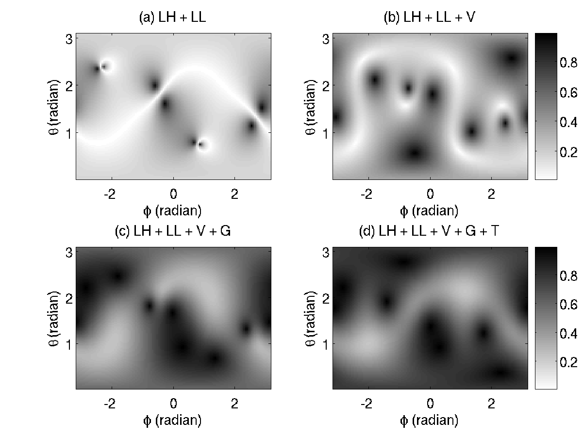
Figure 2: Degeneracy of the network response. We show here the inverse of $\mathrm{cond}\>{(}\mathbf{\Pi})$ for various detector networks (the abbreviated detector names are listed in Table 1). The brighter regions of the sky correspond to the large conditioning number $\mathrm{cond}\>{(}\mathbf{\Pi})$. The fraction of the sky where $1/\mathrm{cond}\>{(}\mathbf{\Pi})<0.1$ is (a) $25\%$ (b) $4.5\%$ (c) $\sim 0\%$ (d) $\sim 0\%$. Since the LIGO detectors are almost aligned and they show the largest percentage of degeneracy.

Connection to the antenna pattern function

— Interestingly, the SVs of $\mathbf{D}$ and $\mathbf{F}\equiv[\mathbf{f}\>\mathbf{f}^{*}]$ coincide. This can be seen from the following relationships we directly obtained from the definitions in Eqs. (17), (18) and (20)

$$\begin{bmatrix}\tilde{\mathbf{f}}&\tilde{\mathbf{f}}^{*}\end{bmatrix}=\mathbf{D}\begin{bmatrix}t_{+}&t_{-}^{*}\\ t_{-}&t_{+}^{*}\end{bmatrix}=\mathbf{F}\begin{bmatrix}|t_{+}|&|t_{-}|\\ |t_{-}|&|t_{+}|\end{bmatrix}.$$ (40)

The matrix $\mathbf{F}$ can be obtained from $\mathbf{D}$ by a unitary transformation. Both matrices share the same singular spectrum. We can therefore write

$$\sigma^{2}_{2}=\sum_{j=1}^{d}|f[j]|^{2}-\left|\sum_{j=1}^{d}f[j]\right|^{2}.$$ (41)

When $\sigma_{2}\sim 0$, we thus have $|\mathbf{f}_{+}\times\mathbf{f}_{\times}|^{2}\sim 0$ where $\mathbf{f}_{+}\equiv\Re[\mathbf{f}]$ and $\mathbf{f}_{\times}\equiv\Im[\mathbf{f}]$ are the network antenna pattern vectors. This means that at such sky locations, the antenna pattern vectors get aligned even if the detectors in the network are misaligned. In other words, despite the considered network is composed of misaligned detectors, it acts as a network of aligned detectors at those sky locations. (Of course, for perfectly co-aligned detectors, $\mathbf{f}_{+}\propto\mathbf{f}_{\times}$ at all sky locations.) Networks with many different detectors having different orientations are less likely to be degenerate. This is confirmed in Fig. 2 where we see that the size of the degenerate sky patches reduces when the number of detector with varied orientations increases. For instance, with a network of LL-LH-G-V, (assuming they have identical noise spectrum), it goes to zero.

V Network likelihood analysis: GW polarization plane and synthetic streams

Generally speaking, a signal detection problem amounts to testing the null hypothesis ($H_{0}$) (absence of signal in the data) vs the alternate hypothesis ($H_{1}$) (presence of signal in the data). Due to the presence of noise, two types of errors occur: false dismissals (decide $H_{0}$ when $H_{1}$ is present) and false alarms (decide $H_{1}$ when $H_{0}$ is present). There exist several objective criteria to determine the detection procedure (or statistic) which optimizes the occurrence of these errors. We choose the Neyman-Pearson (NP) approach which minimizes the number of false dismissals for a fixed false alarm rate. It is easily shown that for simple problems, the likelihood ratio (LR) is NP optimal. However, when the signal depends upon unknown parameters, the NP optimal (uniformly over all allowed parameter values) statistic is not easy to obtain. Indeed for most real-world problems, it does not even exist. However, the generalized likelihood ratio test (GLRT) Kay (1998) have shown to give sensible results and hence is widely used. In the GLRT approach, the parameters are replaced by their maximum likelihood estimates. In other words, the GLRT approach uses the maximum likelihood ratio as the statistic. Here, we opt for such a solution.

As a first step, we consider the simplified situation where all detectors have independent and identical instrumental noises and this noise is white and Gaussian with unit variance. We will address the colored noise case later in Sec. V.4.

In this case, the logarithm of the network likelihood ratio (LLR) is given by

$$\Lambda(\mathbf{x})=-\big{\|}\mathbf{x}-\mathbf{s}\big{\|}^{2}+\big{\|}\mathbf{x}\big{\|}^{2},$$ (42)

where $\big{\|}\cdot\big{\|}^{2}$ is the Euclidean norm (here in $\mathbb{R}^{Nd}$) and we omitted an unimportant factor $1/2$. The network data vector $\mathbf{x}$ is constructed on the similar lines as that of the network response $\mathbf{s}$, i.e. first, it stacks the data from all the detectors into $\mathbf{x}^{T}=[\mathbf{x}_{1}^{T},\mathbf{x}_{2}^{T},\ldots\mathbf{x}_{d}^{T}]$ and then at each detector, the data is time-shifted to account for the delay in the arrival time $\mathbf{x}_{j}=\{x_{j}[k]=x_{j}(t_{k}+\tau_{j}),t_{k}=t_{s}k\mathrm{~{}~{}and~{}~{}}k=0\ldots N-1\}$.

V.1 Maximization over extrinsic parameters: scaling factors and phase shifts

Following the GLRT approach, we maximize the network LLR $\Lambda$ with respect to the parameters of $\mathbf{s}$. We replace $\mathbf{s}$ by its model as given in Eq. (21) and consider at first the maximization with respect to the extrinsic parameters $\mathbf{p}$.

V.1.1 Least-square fit

The maximization of the network LLR over $\mathbf{p}$ amounts to fitting a linear signal model to the data in least square (LS) sense, viz.

$$\text{minimize}\quad-\Lambda(\mathbf{x})+\big{\|}\mathbf{x}\big{\|}^{2}=\big{\|}\mathbf{x}-\mathbf{\Pi}\mathbf{p}\big{\|}^{2}\quad\text{over $\mathbf{p}$}.$$ (43)

This LS problem is easily solved using the pseudo-inverse $\mathbf{\Pi}^{\#}$ of $\mathbf{\Pi}$ Golub and Van Loan (1996). The estimate of $\mathbf{p}$ is then given by

$$\hat{\mathbf{p}}=\mathbf{\Pi}^{\#}\mathbf{x}\,.$$ (44)

The pseudo-inverse can be expressed using the SVD of $\mathbf{\Pi}$ as $\mathbf{\Pi}^{\#}=\mathbf{V}_{\Pi}\mathbf{\Sigma}_{\Pi}^{-1}\mathbf{U}_{\Pi}^{H}$ (note that $\mathbf{\Pi}^{\#}$ is always defined since we use the compact SVD restricted to non-zero SVs).

Substituting Eq. (44) in Eq. (43), we get the LS minimum to be

$$-\hat{\Lambda}(\mathbf{x})+\big{\|}\mathbf{x}\big{\|}^{2}=\big{\|}\mathbf{x}-\mathbf{U}_{\Pi}\mathbf{U}_{\Pi}^{H}\mathbf{x}\big{\|}^{2},$$ (45)

where we used $\mathbf{V}_{\Pi}^{H}\mathbf{V}_{\Pi}=\mathbf{I}_{r}$. Eq. (45) can be further simplified into

$$\hat{\Lambda}(\mathbf{x})=\big{\|}\mathbf{U}_{\Pi}^{H}\mathbf{x}\big{\|}^{2}.$$ (46)

It is interesting to note that the operator $\mathbf{U}_{\Pi}\mathbf{U}_{\Pi}^{H}$ is a (orthogonal) projection operator onto the signal space (over the range of $\mathbf{\Pi}$) i.e. $\mathbf{U}_{\Pi}\mathbf{U}_{\Pi}^{H}\mathbf{\Pi}=(\mathbf{\Pi}\mathbf{\Pi}^{\#})\mathbf{\Pi}=\mathbf{\Pi}$.

V.1.2 Signal-to-noise ratio

The signal-to-noise ratio (SNR) measures the level of difficulty for detecting a signal in the noise. In the present case, along with the amplitude and duration of the incoming GW, the network SNR also depends on the relative position, orientation of the source with respect to the network. Therefore, the SNR should incorporate all these aspects. A systematic way to define the SNR is to start from the statistic.

Let the SNR $\rho$ of an injected GW chirp $\mathbf{s}_{0}=\mathbf{\Pi}\mathbf{p_{0}}$ be

$$\rho^{2}\equiv\hat{\Lambda}(\mathbf{s}_{0}).$$ (47)

Note that in this expression, the matrix $\mathbf{\Pi}$ in the statistic and in $\mathbf{s}_{0}$ are the same. Using the SVD of $\mathbf{\Pi}$ and the property of the projection operator $\mathbf{U}_{\Pi}^{H}\mathbf{U}_{\Pi}=\mathbf{I}_{r}$, we get $\rho^{2}=\big{\|}\mathbf{s}_{0}\big{\|}^{2}$. The SNR is equal to the “signal energy” in the network data as defined in Eq. (22). Thus, the SNR $\rho$ scales as $\sqrt{N}$ as expected and it depends on the source direction, polarization and network configuration through the gain factor $\big{\|}\mathbf{\tilde{f}}\big{\|}$ . Fig. 3 illustrates how this factor varies for the network formed by the two LIGO detectors and Virgo. Fig. 3 displays the ratio $\rho/\rho_{\mathrm{best}}$ between the global SNR (obtained with a coherent analysis) and the largest individual SNR (obtained with the best detector of the network). The panels (a) and (b) are associated to the “worst” (minimum over all polarizations angles $\epsilon$ and $\psi$) and “best” (maximum) cases respectively. Ideally, when the detectors are aligned, the enhancement factor is expected to be $\sqrt{d}$ ($\approx 1.73$ in the present case). In the best case, the enhancement is $\gtrsim 1.7$ for more than half of the sky ($94\%$ of the sky when $\gtrsim 1.4$). In the worst case, the SNR enhancement is $1.28$ at most and $8.5\%$ of the sky gets a value $\gtrsim 1.1$.

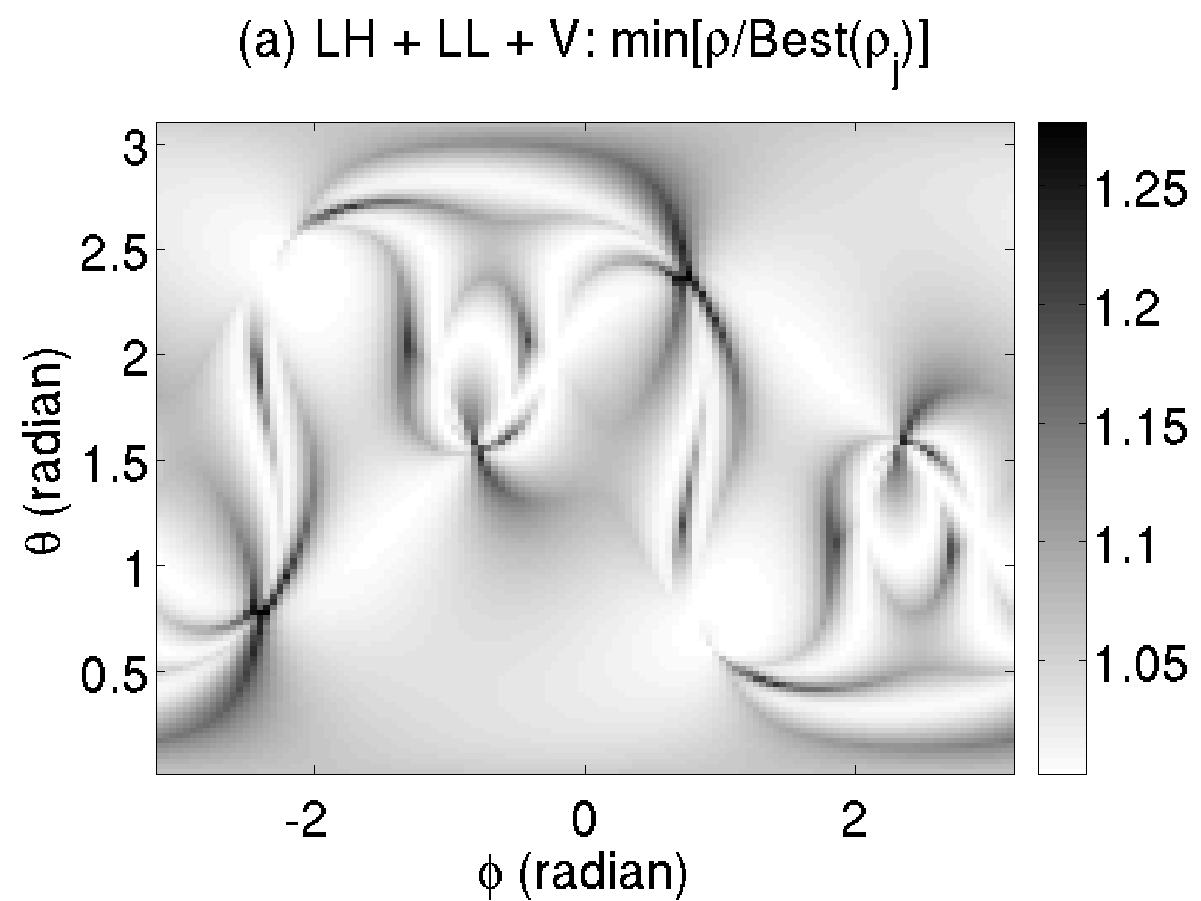
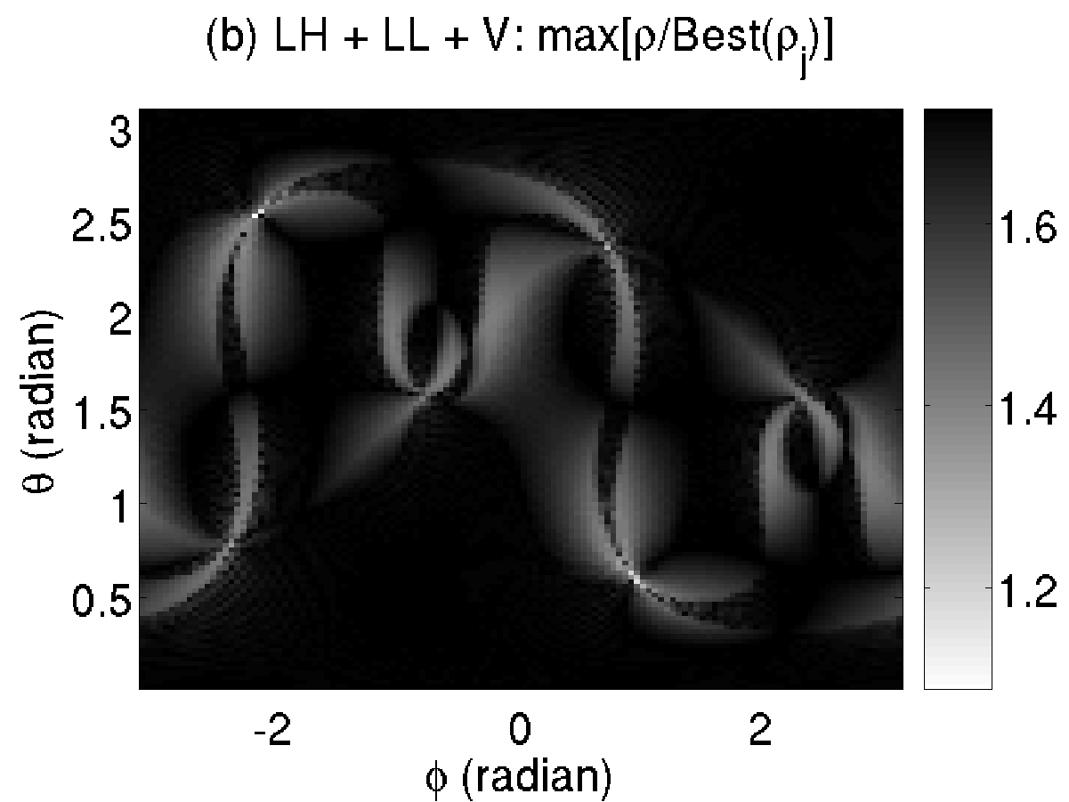
Figure 3: Benefits of a coherent network analysis (SNR enhancement). We display the polar maps of the following quantities for the LL-LH-V network (a) $\min_{\psi,\epsilon}\rho/\rho_{\mathrm{best}}$ and (b) $\max_{\psi,\epsilon}\rho/\rho_{\mathrm{best}}$. Here, $\rho_{\mathrm{best}}$ designates the best SNR of the detectors in the network. The maximum, minimum are taken over all the polarization angles $\{\psi,\epsilon\}$.

V.1.3 From geometrical to physical parameter estimates

The components of $\mathbf{p}$ do not have a direct physical interpretation but as mentioned earlier, they are rather functions of the physical parameters. Following the above discussion, if we assume that we obtained parameter estimates $\hat{\mathbf{p}}$ from the data through Eq. (44), then one can retrieve the physical parameters $A$, $\phi_{0}$, $\epsilon$ and $\psi$ by inverting the non-linear map which links $\mathbf{p}=\left(a~{}t^{*}_{-}~{}~{}a^{*}t_{+}~{}~{}a~{}t^{*}_{+}~{}~{}a^{*}t_{-}\right)^{T}$ to these parameters as given below

$$\hat{A} = (\sqrt{|\hat{p}[1]|}+\sqrt{|\hat{p}[2]|})^{2}\,,$$ (48)

$$\hat{\phi}_{0} = \frac{1}{2}\left[\arg(\hat{p}[1])-\arg(\hat{p}[2])\right]\,,$$ (49)

$$\hat{\psi} = -\frac{1}{4}\left[\arg(\hat{p}[1])+\arg(\hat{p}[2])\right]\,,$$ (50)

$$\hat{\epsilon} = \cos^{-1}\left[\frac{\sqrt{|\hat{p}[2]|}-\sqrt{|\hat{p}[1]|}}{\sqrt{|\hat{p}[2]|}+\sqrt{|\hat{p}[1]|}}\right]\,.$$ (51)

V.1.4 Degeneracy and sensitivity of the estimate to noise

Upper-bounds for the estimation error can be obtained using a perturbative analysis of the LS problem in Eq. (43). A direct use of the result of Golub and Van Loan (1996), Sec. 5.3.8 yields

$$\frac{\|\hat{\mathbf{p}}-\mathbf{p}\|}{\|\mathbf{p}\|}\leq\frac{\sqrt{N}}{\rho}\mathrm{cond}\>{(}\mathbf{\Pi}).$$ (52)

This bound is a worst-case estimate obtained when the noise term which affects the data $\mathbf{x}$ is essentially concentrated along the directions associated to the smallest SV of $\mathbf{\Pi}$. The noise is random and it spans isotropically all $Nd$ dimensions of the signal space. As described above, the space associated to the smallest SV has only 2 dimensions. Therefore, the worst case is very unlikely to occur and the above bound is largely over-estimated on the average. However, it gives a general trend and shows that the estimation goes worst with the conditioning of $\mathbf{\Pi}$.

Regularization techniques seem to give promising results in the context of GW burst detection Klimenko et al. (2005); Mohanty et al. (2006); Rakhmanov (2006). Following this idea, we may consider to “regularize” the LS problem in Eq. (43). To do so, additional information on the expected parameters is required to counterbalance the rank-deficiency. Unfortunately, we don’t expect $\mathbf{p}$ to follow a specific structure. The only sensible prior that can be assumed without reducing the generality of the search is that $\|\mathbf{p}\|$ is likely to be bound (since the GW have a limited amplitude $A$). It is known Neumaier (1998) that this type of prior is associated to the use of the so-called Tykhonov regulator and that we don’t expect significant improvements upon the non-regularized solution.

Probably, one difference might explain why regularization techniques do not work in the present case while it does work for burst detection. We recall that in the burst case, the parameter vector comparable to $\mathbf{p}$ are the samples of the waveform. This vector being a time-series, it is expected to have some structure, in particular it is expected to have some degree of smoothness. The use of this a priori information improves significantly the final estimation.

While regularization will not help for the estimation of the extrinsic parameters, they may be of use to improve the detection statistic. We consider this separate question later in Sec. VII.2.

V.2 Implementation with synthetic streams

In the previous section, we maximize the network LLR with respect to the extrinsic parameters resulting in the statistic $\hat{\Lambda}$ in Eq. (46). Here, we obtain a more simple and practical expression for $\hat{\Lambda}$ which will be useful for maximization over the remaining intrinsic parameters.

From Eqs. (23) and (46), we have

$$\hat{\Lambda}(\mathbf{x})=\big{\|}(\mathbf{U}_{D}\otimes\mathbf{U}_{E})^{H}\mathbf{x}\big{\|}^{2}.$$ (53)

It is useful to reshape the network data $\mathbf{x}$ into a $N\times d$ matrix $\mathbf{X}\equiv[\mathbf{x}_{1}\mathbf{x}_{2}\ldots\mathbf{x}_{d}]$. This operation is inverse to the stack operator $\mathrm{vec}{()}$ defined in Appendix A.

Using a property of the Kronecker product in Eq. (83), we obtain the reformulation

$$\hat{\Lambda}(\mathbf{x})=\big{\|}\mathrm{vec}{(\mathbf{U}_{E}^{H}\mathbf{X}\mathbf{U}_{D}^{*})}\big{\|}^{2}.$$ (54)

There are two possibilities to make this matrix product, each being associated to a different numerical implementation for the evaluation of $\hat{\Lambda}$.

A first choice is to first multiply $\mathbf{X}$ by $\mathbf{U}_{E}^{H}$ and then by $\mathbf{U}_{D}^{*}$. In practice, this means that we first compute the correlation of the data with a chirp template, then we combine the result using weights (related to the antenna pattern functions). This is the implementation proposed in Pai et al. (2001). It is probably the best for cases (like, searches of inspiralling binary chirps) where the number of chirp templates is large (i.e., larger than the number of source locations) and where the correlations with templates are computed once and stored.

The second choice is to first multiply $\mathbf{X}$ by $\mathbf{U}_{D}^{*}$ and then by $\mathbf{U}_{E}^{H}$ which we adopt here. This means that we first compute $\mathbf{Y}\equiv\mathbf{X}\mathbf{U}_{D}^{*}$ which transforms the network data into two $N$-dimensional complex data vectors $[\mathbf{y}_{1},\mathbf{y}_{2}]\equiv\mathbf{Y}$ through an “instantaneous” linear combination. Then, we correlate these vectors with the chirp template. We can consider $\mathbf{y}_{1}$ and $\mathbf{y}_{2}$ as the output of two “virtual” detectors. For this reason, we refer to those as synthetic streams in connection to Sylvestre (2003) who first coined the term for such combinations. Note that, irrespective of the number of detectors, one always gets at most two synthetic streams. We note that though the synthetic streams defined in Sylvestre (2003) are ad-hoc (i.e., they have no relation with the LR), the ones obtained here directly arise from the maximization of the network LLR.

We express the network LLR statistic in terms of the two synthetic streams as

$$\hat{\Lambda}(\mathbf{x})=\frac{1}{N}\left(|\mathbf{e}^{H}\mathbf{y}_{1}|^{2}+|\mathbf{e}^{T}\mathbf{y}_{1}|^{2}+|\mathbf{e}^{H}\mathbf{y}_{2}|^{2}+|\mathbf{e}^{T}\mathbf{y}_{2}|^{2}\right),$$ (55)

where $\mathbf{y}_{l}=\mathbf{X}\mathbf{u}^{*}_{l}$ for $l=1,2$. This expression can be further simplified by using the symmetry (easily seen from Eqs. (33) and (34)),

$$\mathbf{u}_{1}^{*}=\exp(i\delta)\mathbf{u}_{1}\,,\quad\quad\mathbf{u}_{2}^{*}=-\exp(i\delta)\mathbf{u}_{2}\,.$$ (56)

We finally obtain

$$\hat{\Lambda}(\mathbf{x})=\frac{2}{N}(|\mathbf{e}^{H}\mathbf{y}_{1}|^{2}+|\mathbf{e}^{H}\mathbf{y}_{2}|^{2})\,.$$ (57)

The linear combination in each stream is such that the signal contributions from each detector add up constructively. In this sense, synthetic streams are similar to beam-formers used in array signal processing Van Trees (2002).

When the data is a noise free GW chirp, i.e., $\mathbf{x}=\mathbf{s}$, we then have

$$y_{l}[k]=\mathbf{p}^{T}(\mathbf{D}\otimes\mathbf{E}[k])^{T}\mathbf{u}^{*}_{l}=\mathbf{p}^{T}(\sigma_{l}\mathbf{v}^{*}_{l}\otimes\mathbf{E}[k]^{T})\,.$$ (58)

Here, $\mathbf{E}[k]$ represents the $k$-th row of $\mathbf{E}$. Writing explicitly, we have

$$\mathbf{y}_{1} =\frac{\sigma_{1}}{\sqrt{2}}\Re\{q_{1}\mathbf{\tilde{h}}\}e^{i\delta/2}, \mathbf{y}_{2} =\frac{i\sigma_{2}}{\sqrt{2}}\Im\{q_{2}\mathbf{\tilde{h}}\}e^{i\delta/2}\,,$$ (59)

where $q_{1}=(t_{-}e^{-i\delta/2}+t_{+}e^{i\delta/2})^{*}$, $q_{2}=(t_{-}e^{-i\delta/2}-t_{+}e^{i\delta/2})^{*}$ and where $\mathbf{\tilde{h}}$ is as defined in Eq. (16). This shows that the synthetic streams $\mathbf{y}_{l}$ are rescaled and phase shifted copies of the initial GW chirp $\mathbf{\tilde{h}}$ which enhances the amplitude of the signal by the appropriate factor as shown above.

To assess this enhancement, we compute the SNR per synthetic stream as below.

V.2.1 SNR per synthetic streams

The network SNR can be split into the contributions from each synthetic stream i.e. we write $\rho^{2}=\big{\|}\mathbf{\Sigma}_{\Pi}\mathbf{V}_{\Pi}^{H}\mathbf{p}_{0}\big{\|}^{2}$, as

$$\rho^{2}=\rho_{1}^{2}+\rho_{2}^{2},$$ (60)

where we define $\rho_{l}\equiv\sqrt{N}\sigma_{l}\big{\|}(\mathbf{v}_{l}\otimes\mathbf{I}_{2})^{H}\mathbf{p}_{0}\big{\|}/2$ for $l=1,2$. More explicitly, we have

$$\rho_{l}=\frac{\sqrt{N}}{2}\sigma_{l}|q_{l}|A\,.$$ (61)

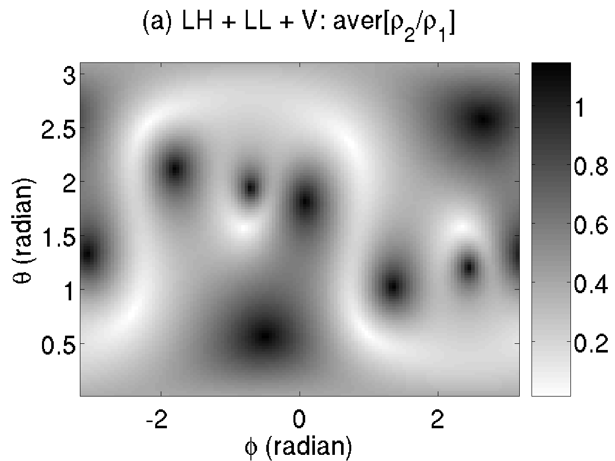
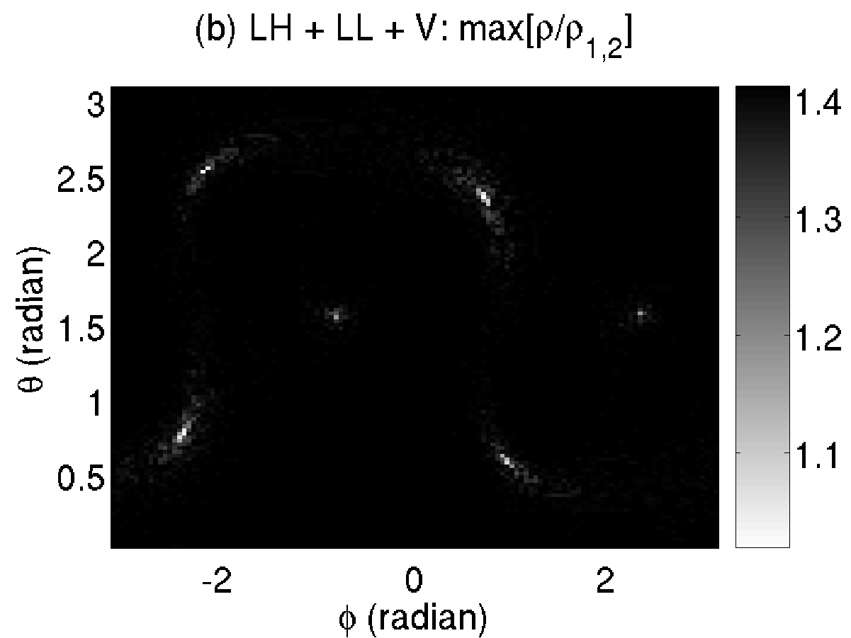
Figure 4: Color online — SNR per synthetic streams and benefits of a coherent network analysis (SNR enhancement). We display the polar maps of the following quantities for the LL-LH-V network: (a) $\langle\rho_{2}/\rho_{1}\rangle_{\psi,\epsilon}$ and (b) $\max_{\psi,\epsilon}\rho/\max_{l}{\rho_{l}}$ . We denote $\rho_{l}$ the SNR of synthetic stream as defined in Eq. (61). The maximum and average are taken over all the polarization angles $\{\psi,\epsilon\}$.

The synthetic streams contributes differently depending on the polarization of the incoming wave. Fig. 4 illustrates this with the network formed by the two LIGO detectors and Virgo.

Let us assume that $\mathbf{p}_{0}$ is randomly oriented. Since $\mathbf{v}_{1}$ and $\mathbf{v}_{2}$ have unit norms, we get the average value $0<\langle\rho_{2}/\rho_{1}\rangle_{\epsilon,\psi}\propto 1/\mathrm{cond}\>{(}\mathbf{\Pi})\leq 1$ for most of the sky as indicated in Fig. 4 (a). Note that this panel matches well with Fig. 2 (b). Thus, on average, $\mathbf{y}_{1}$ contributes more to the SNR than $\mathbf{y}_{2}$. However, the situation may be different depending on the specific polarization state of the wave. Fig. 4 (b) show the maximum of the ratio $\rho/\max_{l=1,2}{\rho_{l}}$ for all polarization angles $\epsilon$ and $\psi$ mostly takes the value $\approx\sqrt{2}$. This implies that for a given direction, one can always find polarization angles where the two synthetic streams contribute equally. This holds true for all the sky locations, except at the degenerate sky locations where $\mathbf{y}_{2}$ does not contribute, hence the SNR ratio is $1$.

Another way to see this is to examine the expression of the SNR difference in terms of the signal and network quantities, namely

$$\rho_{l}^{2}-\rho_{2}^{2}=\frac{NA^{2}}{4}\left(\frac{|\Delta|}{2}\left[\left(\frac{1+\cos^{2}\epsilon}{2}\right)^{2}+\cos^{2}\epsilon\right]\right.\\ \left.+\frac{\big{\|}\mathbf{f}_{+}\big{\|}^{4}-\big{\|}\mathbf{f}_{\times}\big{\|}^{4}}{2|\Delta|}\frac{\sin^{4}\epsilon}{4}\right),$$ (62)

where we have $|\Delta|^{2}=(\big{\|}\mathbf{f}_{+}\big{\|}^{2}+\big{\|}\mathbf{f}_{\times}\big{\|}^{2})^{2}-4\big{\|}\mathbf{f}_{+}\times\mathbf{f}_{\times}\big{\|}^{2}$.

In the simple case of a face-on source, i.e. $\epsilon=0$, and if $\mathbf{f}_{\times}$ is orthogonal to $\mathbf{f}_{+}$ with $\big{\|}\mathbf{f}_{\times}\big{\|}=\big{\|}\mathbf{f}_{+}\big{\|}$, then both synthetic streams carry the same SNR $\rho_{1}=\rho_{2}=\sqrt{N/2}A\big{\|}\mathbf{f}_{+}\big{\|}$. However, for other situations, some other wave polarization would lead the same.

Inversely looking at $\min_{\epsilon,\psi}\rho/\max_{l}\rho_{l}$, it can be shown that one can always find a GW polarization such that one of the synthetic streams does not contribute to the SNR.

V.3 Null streams

V.3.1 Review and relation to synthetic streams

The access to noise only data is crucial in signal detection problem. Such data is not directly available in GW experiments, but the use of multiple detectors allows to access it indirectly using the null streams. The general idea behind the null stream is to construct a data stream from the individual detector streams which nullifies the signature of any incoming GW from a particular direction. Since this signal cancellation is specific to GWs, null streams naturally provide an extra tool to verify that a detected signal is indeed a GW or instead a GW like features mimicked by the detector noise whose detection thus has to be vetoed. This is a powerful check since it does not require detailed information about the potential GW signal under test, except an estimate of its source location. (Note that in practice, the implementation of the veto test may be complicated by the imprecision of the direction of arrival and of the errors of calibration Chatterji et al. (2006)). The existence of null streams has been first identified in Guersel and Tinto (1990) in the case of three detector networks. At present, handful of literature Wen and Schutz (2005); Chatterji et al. (2006) exists on the use of null streams in GW data analysis.

Null streams are usually introduced as a general post-processing of the data independent of the detection of specific GWs. Below, we make this connection in the domain of our formalism. We recall that the network data at a given time (e.g., the first row of the matrix $\mathbf{X}$ introduced in Sec. V.2) is a $d$-dimensional vector in $\mathbb{R}^{d}$. This space is a direct sum of the GW polarization plane and its orthogonal complementary space. We have shown that the GW polarization plane is a $2$-dimensional space, spanned by a pair of orthonormal basis vectors which are associated to the two synthetic streams. The complementary space to the GW polarization plane is a $d-2$ dimensional space and it is spanned by $d-2$ “null vectors”. Similarly to the synthetic streams, the null streams can be constructed from these null vectors. Thus, the numbers of synthetic and null streams sum up to $d$. Nominally, we have $d-2$ null streams. However, when the GW polarization plane degenerates to a $1$-dimensional space ($\sigma_{2}\sim 0$) as explained in Sec. IV.2, the number of null vectors becomes $d-1$. For a two detector network, in the nominal case, there is no null stream as $d-2=0$. However, for degenerate directions, one can construct a null stream. For aligned pair of detectors (as it is almost the case for the two LIGO LH and LL), the fraction of the degenerate sky location is large, see Fig. 2. This null stream would turn out to be useful for vetoing in this case.

In the next section, we explain how the null streams can be obtained numerically in the nominal case. The extension to the degenerate case is straightforward.

V.3.2 Obtaining the null streams numerically

The numerical construction of the null streams can be achieved in various ways. One such approach could be to obtain the full SVD of $\mathbf{D}$ and construct the null streams from the eigen-vectors corresponding to the zero SVs. This approach was taken in Chatterji et al. (2006). Here, we take an alternative approach. We construct the null streams by successive construction of orthonormal vectors via multi-dimensional cross product as described below.

Assuming some direction of arrival, we express any instantaneous linear combination of the time-shifted data (to compensate for different time of arrivals at the detectors’ site with respect to the reference) as

$$\mathbf{y}(\mathbf{x})\equiv\mathbf{X}\mathbf{u},$$ (63)

where the vector $\mathbf{u}\in\mathbb{C}^{d\times 1}$ contains the tap coefficients.

Eq. (63) can be rewritten as

$$\mathbf{y}(\mathbf{x})=\mathrm{vec}{(\mathbf{I}_{N}\mathbf{X}\mathbf{u})}=(\mathbf{u}^{T}\otimes\mathbf{I}_{N})\mathbf{x}.$$ (64)

The vector $\mathbf{u}$ defines a null-stream if $\mathbf{y}(\mathbf{x})=\mathbf{0}_{N}$ whenever $\mathbf{x}$ is a GW. Let us assume that we indeed observe a GW chirp i.e., $\mathbf{x}=\mathbf{s}_{0}\equiv\mathbf{\Pi}\mathbf{p}_{0}$. We thus have

$$\mathbf{y}(\mathbf{s}_{0})=[(\mathbf{u}^{T}\mathbf{U}_{D})\otimes\mathbf{U}_{E}]\mathbf{\Sigma}_{\Pi}\mathbf{V}_{\Pi}^{H}\mathbf{p}_{0}.$$ (65)

If $\mathbf{u}$ is in the null space of $\mathbf{U}_{D}$, the null-stream condition is satisfied for all $\mathbf{p}_{0}$. Since the null space of $\mathbf{U}_{D}$ is orthogonal to its range, an obvious choice for $\mathbf{u}$ is

$$\mathbf{u}=\mathbf{u}_{1}\times\mathbf{u}_{2}=\frac{\mathbf{d}^{*}\times\mathbf{d}}{\sqrt{{\cal D}^{2}-\Delta^{2}}}.$$ (66)

Nominally, $\mathbf{U}_{D}$ is a 2-dimensional plane in $\mathbb{C}^{d}$. Its null space is therefore $d-2$ dimensional. An orthonormal basis of this space can be obtained recursively starting from $\mathbf{u}_{3}=\mathbf{u}$ as defined above and applying the following generalized vector cross-product formula for $n>3$:

$$\mathbf{u}_{n}[i]=\epsilon_{ijkl\ldots m}\mathbf{u}_{1}[j]\mathbf{u}_{2}[k]\mathbf{u}_{3}[l]\ldots\mathbf{u}_{n-1}[m].$$ (67)

Here, $\epsilon_{ijkl\ldots m}$ is the Levi-Civita symbol . The $\mathbf{u}_{n}$ denotes an orthonormal set of $d-2$ vectors, $\{\mathbf{u}_{n},\text{~{}for~{}~{}}3\leq n\leq d\}$. The components of these vectors are the tap coefficients to compute the null-streams. By construction, the resulting null streams are uncorrelated and have the same variance.

To summarize the main features of our formalism. The representation of a GW network response of unmodeled chirp as a Kronecker product between the GW polarization plane and the chirp plane forms the main ingredient of this formalism. Such a representation allows the signal to reveal the degeneracy in a natural manner in the network response. It also evidences the two facets of the coherent network detection problem, namely, the network signal detection via synthetic streams and vetoing via null streams. The coherent formalism developed in Pai et al. (2001) for inspiralling binaries lacked this vetoing feature due to the difference in the signal representation.

In the rest of this paper, we do not discuss/demonstrate the null streams applied as a vetoing tool to the simulated data. This will be demonstrated in the subsequent work with the real data from the ongoing GW experiments.

V.4 Colored noise

The formalism developed till now was exclusively targeted for the white noise case. We assumed that the noise at each detector is white Gaussian. In this subsection, we extend our formalism to the colored noise case. We remind the reader that the main focus of this paper is to develop the coherent network strategy to detect unmodeled GW chirps with an interferometric detector network. Hence, we give more emphasis on the basic formalism and keep the colored noise case with basic minimal assumption: the noise from the different detectors is colored but with same covariance. Based on this ground work, the work is in progress to extend this to the colored noise case with different noise covariances.

Let us therefore assume now that the noise components in each detector are independent and colored, with the same covariance matrix $\mathbf{R}_{0}$. Recall that the covariance matrix of a random vector $\mathbf{a}$ is defined as $\mathbb{E}\left[(\mathbf{a}-\mathbb{E}[\mathbf{a}])(\mathbf{a}-\mathbb{E}[\mathbf{a}])^{H}\right]$ where $\mathbb{E}[.]$ denotes the expectation. From the independence of the noise components, the overall covariance matrix of the network noise vector is then a block-diagonal matrix, where all the blocks are identical and equal to $\mathbf{R}_{0}$: $\mathbf{R}=\text{diag}(\mathbf{R}_{0})\equiv\mathbf{I}_{d}\otimes\mathbf{R}_{0}$.

In this case, the network LLR becomes

$$\Lambda(\mathbf{x})=-\big{\|}\mathbf{x}-\mathbf{\Pi}\mathbf{p}\big{\|}_{\mathbf{R}^{-1}}^{2}+\big{\|}\mathbf{x}\big{\|}_{\mathbf{R}^{-1}}^{2},$$ (68)

where the notation $\big{\|}\cdot\big{\|}_{\mathbf{R}^{-1}}^{2}$ denotes the norm induced by the inner product associated to the covariance matrix ${\mathbf{R}^{-1}}$, i.e., $\big{\|}\mathbf{a}\big{\|}_{\mathbf{R}^{-1}}^{2}=\mathbf{a}^{H}\mathbf{R}^{-1}\mathbf{a}$.

Introducing the whitened version $\tilde{\mathbf{\Pi}}=\mathbf{R}^{-1/2}\mathbf{\Pi}$ and $\tilde{\mathbf{x}}=\mathbf{R}^{-1/2}\mathbf{x}$ of $\mathbf{\Pi}$ and $\mathbf{x}$ respectively, Eq. (68) can be rewritten as

$$\Lambda(\mathbf{x})=-\big{\|}\tilde{\mathbf{x}}-\tilde{\mathbf{\Pi}}\mathbf{p}\big{\|}^{2}+\big{\|}\tilde{\mathbf{x}}\big{\|}^{2}.$$ (69)

which is similar to Eq. (42) where all the quantities are replaced by their whitened version. Thus, the maximization of $\Lambda(\mathbf{x})$ with respect to the extrinsic parameters $\mathbf{p}$ will follow the same algebra as that derived in V. However, for the sake of completeness, we detail it below.

Following Sec. V, maximizing $\Lambda(\mathbf{x})$ with respect to the extrinsic parameters $\mathbf{p}$ leads to

$$\hat{\mathbf{p}}=\tilde{\mathbf{\Pi}}^{\#}\tilde{\mathbf{x}},$$ (70)

where $\tilde{\mathbf{\Pi}}^{\#}$ is the pseudo-inverse of $\tilde{\mathbf{\Pi}}$. Expressing this pseudo-inverse by means of the SVD of $\tilde{\mathbf{\Pi}}$ as $\tilde{\mathbf{\Pi}}^{\#}=\mathbf{V}_{\tilde{\Pi}}\mathbf{\Sigma}_{\tilde{\Pi}}^{-1}\mathbf{U}_{\tilde{\Pi}}^{H}$ and introducing Eq. (70) into Eq. (69) provides the new statistic

$$\hat{\Lambda}(\mathbf{x})=\big{\|}\mathbf{U}_{\tilde{\Pi}}^{H}\tilde{\mathbf{x}}\big{\|}^{2}.$$ (71)

Now, from the definition of $\mathbf{\Pi}$ and the specific structure of $\mathbf{R}$, it is straightforward to see that

$$\tilde{\mathbf{\Pi}}=\mathbf{R}^{-1/2}(\mathbf{D}\otimes\mathbf{E})=\mathbf{D}\otimes(\mathbf{R}_{0}^{-1/2}\mathbf{E})=\mathbf{D}\otimes\tilde{\mathbf{E}},$$ (72)

where we have introduced the whitened version $\tilde{\mathbf{e}}=\mathbf{R}_{0}^{-1/2}\mathbf{e}$ of the chirp signal and the corresponding matrix $\tilde{\mathbf{E}}=[\tilde{\mathbf{e}}~{}\tilde{\mathbf{e}}^{*}]/2$.

For the white noise case, the statistic (71) can then be rewritten in terms of the SVD of the matrices $\mathbf{D}$ and $\tilde{\mathbf{E}}$:

$$\hat{\Lambda}(\mathbf{x})=\big{\|}(\mathbf{U}_{D}\otimes\mathbf{U}_{\tilde{E}})^{H}\tilde{\mathbf{x}}\big{\|}^{2}.$$ (73)

The computation of $\mathbf{U}_{\tilde{E}}$ is similar to the computation of $\mathbf{U}_{\tilde{E}}$. Furthermore, if we note that $\tilde{\mathbf{e}}^{T}\tilde{\mathbf{e}}\simeq 0$, and if we assume that $\tilde{\mathbf{e}}^{H}\tilde{\mathbf{e}}=N$, it turns out that $\mathbf{U}_{\tilde{E}}=2\tilde{\mathbf{E}}/\sqrt{N}=2\mathbf{R}_{0}^{-1/2}\mathbf{E}/\sqrt{N}$. Using the property of the Kronecker product in Eq. (83), we then obtain

$$\hat{\Lambda}(\mathbf{x})=\big{\|}\mathrm{vec}{(\mathbf{E}^{H}\tilde{\tilde{\mathbf{X}}}\mathbf{U}_{D}^{*})}\big{\|}^{2},$$ (74)

where the matrix $\tilde{\tilde{\mathbf{X}}}=[\tilde{\tilde{\mathbf{x}}}_{1}\tilde{\tilde{\mathbf{x}}}_{2}\dots\tilde{\tilde{\mathbf{x}}}_{d}]$ contains the data vector from each detector whitened twice: $\tilde{\tilde{\mathbf{x}}}_{j}=\mathbf{R}^{-1/2}\tilde{\mathbf{x}}_{j}=\mathbf{R}^{-1}\mathbf{x}_{j}$.

As this expression is similar to the white noise case, we can form two synthetic streams $[\tilde{\tilde{\mathbf{y}}}_{1},\tilde{\tilde{\mathbf{y}}}_{2}]=\tilde{\tilde{\mathbf{X}}}\mathbf{U}_{D}^{*}$ and use them to express the LLR statistic as

$$\hat{\Lambda}(\mathbf{x})=\frac{2}{N}(|\mathbf{e}^{H}\tilde{\tilde{\mathbf{y}}}_{1}|^{2}+|\mathbf{e}^{H}\tilde{\tilde{\mathbf{y}}}_{2}|^{2}).$$ (75)

In this expression, the only difference with the white noise LLR of (57) comes from the computation of the synthetic streams $\tilde{\tilde{\mathbf{y}}}_{1}$ and $\tilde{\tilde{\mathbf{y}}}_{2}$ which are obtained after double-whitening the data.

VI Maximization over the intrinsic parameters

In the previous section, we maximized the network LLR over the extrinsic parameters of the signal model, assuming that the remaining parameters (the source location angles $\phi$ and $\theta$ and the phase function $\varphi(\cdot)$) were known.

By definition, the intrinsic parameters modify the network LLR non-linearly. For this reason, the maximization of $\hat{\Lambda}$ over these parameters is more difficult. It cannot be done analytically and must be performed numerically, for instance with an exhaustive search of the maximum by repeatedly computing $\hat{\Lambda}$ over the entire range of possibilities.

While the exhaustive search can be employed for the source location angles, it is not applicable to the chirp phase function, which requires a specific method. For the single detector case, we had addressed this issue in Chassande-Mottin and Pai (2006) with an original maximization scheme which is the cornerstone of the best chirplet chain (BCC) algorithm. Here, we use and adapt the principles of BCC to the multiple detector case.

VI.1 Chirp phase function

Let us examine first the case of the detection of inspiralling binary chirps. In this case, the chirp phase is a prescribed function of a small number of parameters i.e., the masses and spins of the binary stars. The maximization over those is performed by constructing a grid of reference or template waveforms which are used to search the data. This grid samples the range of the physical parameters. This sampling must be accurate (the template grid must be tight) to avoid missing any chirp.

Tight grid of templates can be obtained in the non-parametric case (large number of parameters) i.e., when the chirp is not completely known. We have shown in Chassande-Mottin and Pai (2006) how to construct a template grid which covers entirely the set of smooth chirps i.e., chirps whose frequency evolution has some regularity as described in Sec. II.2.2. In the next section, we briefly describe this construction.

VI.1.1 Chirplet chains: tight template bank for smooth chirps

We refer to the template forming this grid as chirplet chain (CC). These CCs are constructed on a simple geometrical idea: a broken line is a good approximation of a smooth curve. Since the frequency of a smooth chirp follows a smooth frequency vs. time curve, we construct templates that are broken lines in the time-frequency (TF) plane.

More precisely, CC are defined as follows. We start by sampling the TF plane with a regular grid consisting of $N_{t}$ time bins and $N_{f}$ frequency bins. We build the template waveforms like a puzzle by assembling small chirp pieces which we refer to as chirplets. A chirplet is a signal with a frequency joining linearly two neighboring vertices of the grid. The result of this assembly is a chirplet chain i.e., a piecewise linear chirp. Since we are concerned with continuous frequency evolution with bounded variations, we only form continuous chains.

We control the variations of the CC frequency. The frequency of a single chirplet does not increase or decrease more than $N_{r}^{\prime}$ frequency bins over a time bin. Similarly, the difference of the frequency variations of two successive chirplets in a chain does not increase or decrease more than $N_{r}^{\prime\prime}$ frequency bins.

The CC grid is defined by four parameters namely $N_{t}$, $N_{f}$, $N^{\prime}_{r}$ and $N^{\prime\prime}_{r}$. Those are the available degrees of freedom we can tune to make the CC grid tight. A template grid is tight if the network ambiguity $\hat{\Lambda}(\mathbf{s};\varphi^{\prime})\propto|{\mathbf{e}^{\prime}}^{H}\mathbf{y}_{1}(\mathbf{s})|^{2}+|{\mathbf{e}^{\prime}}^{H}\mathbf{y}_{2}(\mathbf{s})|^{2}$ which measures the similarity between an arbitrary chirp (of phase $\varphi$) and its closest template (of phase $\varphi^{\prime}$), is large enough and relatively closed to the maximum (when $\varphi^{\prime}=\varphi$).

As stated in Eq. (59), in presence of a noise free GW chirp, the synthetic streams $\mathbf{y}_{l}(\mathbf{s})$ are rescaled and phase shifted copies of the initial GW chirp $\mathbf{s}$. Therefore, we treat the network ambiguity as a sum of ambiguities from two virtual detectors where each terms in $\hat{\Lambda}(\mathbf{s};\varphi^{\prime})$ is the ambiguity computed in the single detector case. An estimate of the ambiguity has been obtained in Chassande-Mottin and Pai (2006) for this case. It can thus be directly reused to compute $\hat{\Lambda}(\mathbf{s};\varphi^{\prime})$.

The bottom line is that the ratio of the ambiguity to its maximum for the network case remains unaltered as compared to the single detector case and thus same for the tight grid conditions. In conclusion, the rules (which we won’t repeat here) established in Chassande-Mottin and Pai (2006) to set the search parameters can also be applied here.

VI.1.2 Search through CCs in the time-frequency plane: best network CC algorithm

We have now to search through the CC grid to find the best matching template, i.e., which maximizes $\max_{\text{all CCs $\varphi^{\prime}$}}\hat{\Lambda}(\mathbf{x};\varphi^{\prime})$. Counting the number of possible CCs to be searched over is a combinatorial problem. This count grows exponentially with the number of time bins $N_{t}$. In the situation of interest, it reaches prohibitively large values. The family of CCs cannot be scanned exhaustively and the template based search is intractable.

In Chassande-Mottin and Pai (2006), we propose an alternative scheme yielding a close approximation of the maximum for the single detector statistic. When applied to the network, the scheme demands to reformulate the network statistic in the TF plane. The TF plane offers a natural and geometrically simple representation of chirp signals which simplifies the statistic. It turns out that the resulting statistic falls in a class of objective functions where efficient combinatorial optimization algorithms can be used. We now explain this result in more detail.

We use the TF representation given by the discrete Wigner-Ville (WV) distribution Chassande-Mottin and Pai (2005) defined for the time series $x[n]$ with $n=0,\ldots,N-1$ as

$$w_{x}(n,m)\equiv\sum_{k=-k_{n}}^{+k_{n}}x[\lfloor n+k/2\rfloor]x^{*}[\lfloor n-k/2\rfloor]\,e^{-2\pi imk/(2N)},$$ (76)

with $k_{n}\equiv\min\{2n,2N-1-2n\}$, where $\lfloor\cdot\rfloor$ gives the integer part. The arguments of $w_{x}$ are the time index $n$ and the frequency index $m$ which correspond, in physical units, to the time $t_{n}=t_{s}n$ and the frequency $\nu_{m}=\nu_{s}m/(2N)$ for $0\leq m\leq N$ and $\nu_{m}=\nu_{s}(N-m)/(2N)$ for $N+1\leq m\leq 2N-1$.

The above WV distribution is a unitary representation. This means that the scalar products of two signals can be re-expressed as scalar products of their WV. Let $x_{1}[n]$ and $x_{2}[n]$ be two time series. The unitarity property of $w_{x}$ is expressed by the Moyal’s formula as stated below

$$\left|\sum_{n=0}^{N-1}x_{1}[n]\,x_{2}^{*}[n]\right|^{2}=\frac{1}{2N}\sum_{n=0}^{N-1}\sum_{m=0}^{2N-1}w_{x_{1}}(n,m)\,w_{x_{2}}(n,m).$$ (77)

Applying this property to the network statistic in Eq. (57), we get

$$\hat{\Lambda}(\mathbf{x})=\frac{1}{N^{2}}\sum_{n=0}^{N-1}\sum_{m=0}^{2N-1}w_{y}(n,m)w_{e}(n,m).$$ (78)

where $w_{y}=w_{y_{1}}+w_{y_{2}}$ combines the individual WVs of the two synthetic streams.

In order to compute $\hat{\Lambda}(\mathbf{x})$, we need to have a model for $w_{e}$. We know that the WV distribution of a linear chirp (whose frequency is a linear function of time) is essentially concentrated in the neighborhood of its instantaneous frequency Chassande-Mottin and Pai (2005). We assume that it also holds true for an arbitrary (non-linear) chirp. Applying this approximation to the WV $w_{e}$ of the template CC in Eq. (78), we get

$$w_{e}(n,m)\approx 2N\>\delta(m-m_{n}),$$ (79)

where $m_{n}$ denotes the nearest integer of $2T\>\nu(t_{n})$ and $\nu$ is the instantaneous frequency of the CC.

Thus, substituting in Eq. (78), we obtain the following reformulation of the network statistic

$$\hat{\Lambda}(\mathbf{x})=\frac{2}{N}\sum_{n=0}^{N-1}w_{y}(n,m_{n}).$$ (80)

The maximization of $\hat{\Lambda}(\mathbf{x})$ over the set of CC amounts to finding the TF path that maximizes the integral Eq. (80), which is equivalent to a longest path problem in the TF plane. This problem is structurally identical to the single detector case (the only change is the way we obtain the TF map). We can therefore essentially re-use the scheme proposed earlier for this latter case. The latter belongs to a class of combinatorial optimization problems where efficient (polynomial time) algorithms exist. We use one such algorithm, namely, the dynamic programming.

In conclusion, the combination of the two ingredients namely the synthetic streams and the phase maximization scheme used in BCC allows us to coherently search the unmodeled GW chirps in the data of GW detector network. We refer to this procedure as the best network CC (BNCC) algorithm.

VI.2 Source sky position

As we are performing maximization successively, till now we assume that we know the sky position of the source. Knowing the sky position, we construct the synthetic streams with appropriate direction dependent weight factors, time-delay shifts and carry out the BNCC algorithm for chirp phase detection. In reality, the sky position is unknown. One needs to search through the entire sky by sampling the celestial sphere with a grid and repeating the above procedure for each point on this grid.

VI.3 Time of arrival

Since we process the data streams sequentially and block-wise, the maximization over $t_{0}$ amounts to selecting that block where the statistic arrives at a local maximum (i.e., the maximum of the “detection peak”). The epoch of this block yields an estimate of $t_{0}$. The resolution of the estimate may be improved by increasing the overlap between two consecutive blocks.

VI.4 Estimation of computational cost

We estimate the computational cost of the BNCC search by counting the floating-point operations (flops) required by its various subparts. The algorithm consists essentially in repeating the one-detector search for all sky location angles. Let $N_{\Omega}$ be the number of bins of the sky grid. The total cost is therefore $N_{\Omega}$ times the cost of the one-detector search, which we give in Chassande-Mottin and Pai (2006) and summarize now. The computation of the WV of the two synthetic streams requires $10NN_{f}\log_{2}N_{f}$ flops and the BCC search applied to the combined WV requires $[N+(2N_{r}^{\prime\prime}+1)N_{t}]N_{c}$ flops, where $N_{c}\approx(2N_{r}^{\prime}+1)N_{f}$ is the total number of chirplets. Since this last part of the algorithm dominates, the over-all cost thus scales with

$$C\propto N_{\Omega}[N+(2N_{r}^{\prime\prime}+1)N_{t}](2N_{r}^{\prime}+1)N_{f}\,.$$ (81)

These operations are applied to each blocks (of duration $T$) the data streams. The computational power needed to process the data in real time is thus given by $C/(\mu T)$ where $\mu$ is the overlap between two successive blocks.

VII Results with simulated data and discussion

VII.1 Proof of principle of a full blind search

We present here a proof of principle for the proposed detection method. For this case study, we consider a network of three detectors placed and oriented like the existing Virgo and the two four-kilometer LIGO detectors. The coordinates and orientation of these detectors can be found in Table 1. We assume a simplified model for detector noise which we generate independently for each detector, using a white Gaussian noise. Fig. 5 illustrates the possibility of a “full blind” search in this situation. This means that we perform the detection jointly with the estimation of the GW chirp frequency and the source sky location.

VII.1.1 Description of the test signal

Because of computational limitation, we restrict this study to rather short chirps of $N=256$ samples, i.e., a chirp duration $T=250$ ms assuming a sampling rate of $\nu_{s}=1024$ Hz. The chirp frequency follows a random time evolution which however satisfies chirping rate constraints. We make sure that the first and second derivatives of the chirp frequency are not larger than $F^{\prime}=9.2$ kHz/s and $F^{\prime\prime}=1.57$ MHz/s² respectively. The chosen test signal has about $50$ cycles. This is a larger number than what is considered typically for burst GWs ( $\sim$ 10).

As a comparison with a well-known physical case, an inspiralling (equal mass) binary with total mass $M=11M_{\odot}$ reaches the same maximum frequency variations at the last stable circular orbit. (Binary chirps with larger total mass also satisfy these chirping rate limits).

We set the SNR to $\rho=20$. The chirp is injected at the sky position $\phi=2.8$ rad and $\theta=0.4$ rad where the contributions of the individual detectors are comparable, namely the individual SNR are $10.4$, $10.15$ and $13.77$ for Virgo, LIGO Hanford and LIGO Livingstone respectively.

VII.1.2 Search parameters

We search through the set of CCs defined over a TF grid with $N_{t}=128$ time intervals and $N=N_{f}=256$ frequency bins (using $f_{s}=2048$ Hz). We set the regularity parameters to $N_{r}^{\prime}=9$ and $N_{r}^{\prime\prime}=3$, consistent to the above chirping rate limits.

We select an ad-hoc sky grid by dividing regularly the full range of the source localization angles $\theta$ and $\phi$ into 128 bins. The resulting grid has therefore a total of $N_{\Omega}=16384$ bins. This is probably much finer than is required to perform the detection without missing candidate. However, this oversampling leads to precise likelihood sky maps which helps to diagnose the method. With this parameter choice, the estimated computational power required to analyzed the data in real time is of $2.8$ TFlops, assuming an overlap of $\mu=50\%$ between successive data blocks. Because of the crude choice for the sky grid, this requirement is probably over-estimated.

The result of the search is displayed in Fig. 5 where we see that the injection is recovered both in sky position and frequency evolution. The source position is estimated at $\hat{\phi}=2.8$ rad and $\hat{\theta}=0.39$ rad.

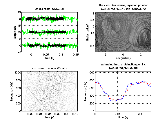
Figure 5: Color online — Coherent detection/estimation of a “random” chirp with network of three GW antennas. In the data of three GW antennas (the two LIGO and Virgo), we inject (a) a “random” GW chirp emitted from a source at the position marked with a “+” at $\phi=2.8$ rad and $\theta=0.4$ rad. We perform a full sky search using the best network chirplet chain algorithm. It produces a likelihood landscape (b) where we select the maximum. This is the detection point and it is indicated with “$\times$”. In (c) we show the combined WV distribution of the synthetic streams at the detection point. In (d), we compare the exact frequency of the chirp (solid/blue) with the estimation (dashed/red) obtained at the detection point.

VII.2 Regularized variants

As shown in Sec. V.2.1, the SNR carried by the synthetic stream is proportional to the corresponding SV. When the GW polarization plane is degenerate (i.e., when $\sigma_{2}$ is small), the second synthetic stream contains almost only noise. We thus don’t lose information if we suppress its contribution from the statistic. This is the basic idea of Klimenko et al. in Klimenko et al. (2005).

We have seen that the estimation of the extrinsic parameters is an ill-posed least-square problem in those cases. Suppressing the contribution of the second synthetic stream amounts to regularizing this problem Klimenko et al. (2005). In practice, this regularization can be done in various ways, corresponding to well-identified schemes.

A first possibility is to suppress the contribution of the second synthetic stream when the conditioning number of $\mathbf{\Pi}$ is too large (i.e., exceeds a given threshold). This scheme is referred to as truncated SVD Neumaier (1998). A second possibility is to balance (divide) the contribution of the second synthetic stream by the conditioning number. This is referred to as the Tykhonov approach Neumaier (1998) and it was proposed for regularizing burst searches in Rakhmanov (2006).

In Fig. 6, we compare the likelihood landscape and frequency estimate obtained with the standard statistic and its regularized version using the Tykhonov approach. Visually, the regularization improves the contrast and concentration of the likelihood landscape around the injection point. This can be assessed more quantitatively with the contrast defined as the ratio of the likelihood landscape extremes. This contrast is improved by about $10\%$ for the regularized statistic as compared to the standard version. It is also interesting to compare the “width” of the detection peak obtained with the two statistic. To do this, we measure the solid angle of the the sky region where the statistic is larger than $90\%$ of the maximum. This angle is reduced by a factor of $\sim$ 6 when computed with the regularized statistic. There is however no major improvement of the frequency estimate. More generally, it is unclear whether the regularized statistic performs better than the standard one.

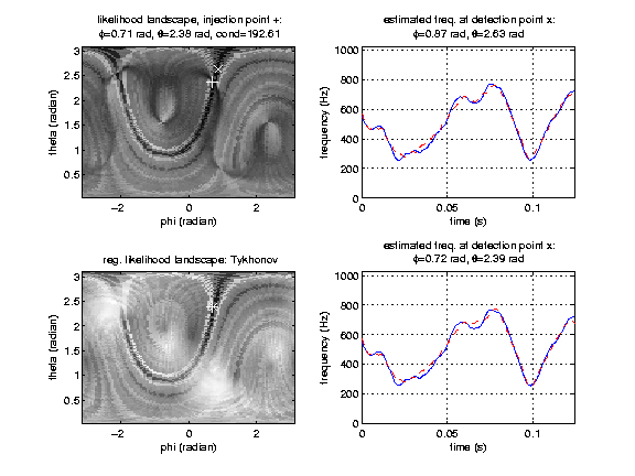
Figure 6: Color online — Coherent detection/estimation of a “random” chirp with network of three GW antennas. Standard and regularized statistic. We compare the likelihood landscape (left) and frequency estimation (right) obtained using the standard (top) and Tykhonov-regularized (bottom) versions of the network statistic. The test signal is a “random” GW chirp injected at the sky location marked with a “+”. This location has been chosen because of the associated large value of the conditioning number, namely $\mathrm{cond}\>{(}\mathbf{\Pi})\approx 192$.

VIII Concluding remarks

The coherent detection of unmodeled chirps with a network of GW have features and issues in common with the burst one. In particular, the same geometrical objects play a key role. While the noise spans the whole $d$ dimensional data space, GW signals (chirps or burst) only belong to a two-dimensional (one dimension per GW polarizations) subspace, the GW polarization plane. Detecting GWs amounts to checking whether the data has significant components in this plane or not. To do so, we compute the projections of the data onto a basis of the GW polarization plane. In practice, this defines two instantaneous linear mixtures of the individual detector data which we refer to as synthetic streams. Those may be considered as the output data of “virtual” detectors. This combination is such that the GW contributions from each real detector add constructively. The GW signature thus has a larger amplitude in the synthetic streams while the noise variance is kept at the same level.

The coherent detection amounts to looking for an excess in the signal energy in one or both synthetic streams (depending on the GW polarization model). This provides a generic and simple procedure to produce a coherent detection pipeline from a one detector pipeline. In the one detector case, the BCC search performs a path search in a time-frequency distribution of the data. In the multiple detector case, the BNCC search now use the joint time-frequency map obtained by summing the time-frequency energy distributions of the two synthetic streams. The approach does not restrict to chirp detection and it can be applied to burst searches Chatterji et al. (2006).

We demonstrated in a simplified situation that the full-sky blind detection of an unmodeled chirp is feasible. This means that the detection is performed jointly to estimate the source location and the frequency evolution. The application of this method to the real data however requires several improvements. First, the method has to be adapted to the case where the detectors have different sensitivities. In this respect, we already obtained first results Rabaste et al. (2007).

We also have to refine the choice of the grid which samples the celestial sphere. In the present work, we select an ad-hoc grid. Clearly, the sky resolution and the bin shape depends on the geometry of the sphere and the location and orientation of the detectors in the considered network. A better grid choice (not too coarse to avoid SNR loses, or and not too fine to avoid using useless computing resources) should incorporate this information keeping the search performance (detection probability and sky resolution) constant. In this respect, we may consider to other parameterizations of the sky location which makes the definition of the sky grid easier, for instance by choosing the time-delays as investigated in Pai et al. (2001). We may also explore hierarchical schemes for the reduction of the computational cost.

The GW polarization plane depends on the detector antenna patterns functions. With the presently available networks, there are significantly large sky regions where the antenna patterns are almost aligned. In this case, the network observes essentially one polarization and is almost insensitive to the other: the GW polarization plane reduces to a one-dimensional space. The information carried by the missing polarization lacks and this makes the estimation of certain parameters ill-posed and hence very sensitive to noise. We can evaluate that the variance of the estimate scales with the condition number of the antenna pattern matrix. When this number (which quantifies in some sense the mutual alignment of the detectors) is large, the estimation is ill-posed and we expect poor results.

This is an important issue for burst detection since it affects significantly the shape of the estimated waveform (and, particularly the regularity of its time evolution). This has motivated the development of regularization schemes which penalize the estimation of non-physical (i.e., irregular) waveforms. We have shown that this is however less of a problem for chirps because of their more constrained model. Ill-conditioning only affects global scaling factors in the chirp model. Unlike bursts, no additional prior is available for regularizing the estimation of these scaling factors.

The data space can be decomposed as the direct sum of the GW polarization plane and its complementary. While GWs have zero components in the latter null space, it is unlikely that instrumental noise (including its non-Gaussian and non-stationary part) will. This motivates the use of null streams (i.e., the projection of the data along a basis of the complementary space) to verify that a trigger is indeed a GW candidate and not an instrumental artifact. Since null streams are inexpensive to compute, we consider to use them to make preemptive cuts in order to avoid the analysis of bad data.

Appendix A Kronecker product: definition and properties

The Kronecker product $\otimes$ transforms two matrices $\mathbf{A}\in\mathbb{C}^{m\times n}$ and $\mathbf{B}\in\mathbb{C}^{p\times q}$ into the following matrix of $\mathbb{C}^{mp\times nq}$ Horn and Johnson (1991)

$$\mathbf{A}\otimes\mathbf{B}\equiv\left[\begin{array}[]{ccc}a_{11}\mathbf{B}&\ldots&a_{1n}\mathbf{B}\\ \vdots&\ddots&\vdots\\ a_{m1}\mathbf{B}&\ldots&a_{mn}\mathbf{B}\end{array}\right].$$ (82)

The Kronecker product is a linear transform and can be considered as a special case of the tensor product. We define the operator $\mathrm{vec}{()}$ to be the stack operator which transforms the matrix into a vector by stacking its columns, i.e. $\mathbf{x}\equiv\mathrm{vec}{(\mathbf{X})}$. In the text, we use the following property:

$$(\mathbf{A}\otimes\mathbf{B})\mathrm{vec}{(\mathbf{X})}=\mathrm{vec}{(\mathbf{B}\mathbf{X}\mathbf{A}^{T})}.$$ (83)

The proof of this property is straightforward.

Appendix B Interferometric detector response in terms of Gel’fand functions

The GW response of a detector to an incoming GW can be obtained by computing the interaction of the wave tensor $W$ with the detector tensor $D$ as follows :

$$s=\sum_{i,j=1}^{3}W^{ij}D_{ij}.$$ (84)

The wave tensor is related to the incoming GW tensor in the TT gauge by $h_{ij}=2W_{ij}$. Both detector and wave tensors are rank 2 STF tensors. Any STF tensor can be expanded in the basis of spin-weighted spherical harmonics of rank 2 and the rank-2 Gel’fand functions provide the corresponding coefficients. Further, they are representation of rotation group SO(3) and provide compact representation for the detector response of any arbitrarily oriented and located detector on Earth which we present in this appendix Dhurandhar and Tinto (1998).

Wave tensor

— The incoming GW tensor in TT gauge is given by

$$h_{ij}^{TT}=(e_{xi}e_{xj}-e_{yi}e_{yj})h_{+}+2(e_{xi}e_{yj})h_{\times},$$ (85)

where ${\bf e_{x}}$ and ${\bf e_{y}}$ are unit vectors along the $x_{w}$ and $y_{w}$ axes in the wave frame; $h_{+}$ and $h_{\times}$ are the two GW polarizations. Let $\hat{m}=({\bf e_{x}}+i{\bf e_{y}})/\sqrt{2}$ be a complex vector in the wave frame. Then, the wave tensor can be written down in terms of $m$ as

$$W^{ij}=\Re[(m^{i}m^{j})^{*}h]\,,$$ (86)

where we used the complex quantity $h=h_{+}+ih_{\times}$ which combines both GW polarizations.

The term $m_{i}m_{j}$ is a STF tensor of rank 2. We choose to work in the detector frame for convenience. Expanding $m_{i}m_{j}$ in terms of spin-weighted spherical harmonics of rank 2, namely ${\cal Y}^{ij}_{2n}$ and the rank-2 Gel’fand functions $T_{mn}(\phi^{\prime}_{e},\theta^{\prime}_{e},\psi^{\prime}_{e})$, we get

$$m^{i}m^{j}=\sqrt{\frac{8\pi}{15}}\sum_{n=-2}^{2}{\cal Y}_{2n}^{ij}T_{2n}(\phi^{\prime}_{e},\theta^{\prime}_{e},\psi^{\prime}_{e})\,,$$ (87)

The angles $(\phi^{\prime}_{e},\theta^{\prime}_{e},\psi^{\prime}_{e})$ are the Euler angles of the rotation operator which transforms the detector coordinates into the wave coordinates.

Substituting Eq. (87) into Eq. (86), we express the wave tensor in terms of the Gel’fand functions as

$$W^{ij}=\sqrt{\frac{8\pi}{15}}~{}\sum_{n=-2}^{2}\Re[h{\cal Y}_{2n}^{ij}T_{-2n}]\,.$$ (88)

Detector tensor

— The detector tensor is

$$D_{ij}=n_{1i}n_{1j}-n_{2i}n_{2j},$$ (89)

where $\mathbf{n}_{1}$ and $\mathbf{n}_{2}$ are the unit vectors along the first and second arms of the interferometer. Recall that we choose the $x_{d}$-axis of the detector frame along the bisector of the two arms. The $y_{d}$-axis is chosen such that $(x_{d},y_{d},z_{d})$ is a right handed coordinate system with $z_{d}$ pointing towards the local zenith. With this choice, we have

$$D_{11}=D_{22}=0\,,\hskip 56.9055ptD_{12}=D_{21}=-1\,.$$ (90)

From Eqs. (89) and (90), the detector response is

$$s=\Re[f^{*}h],$$ (91)

where the complex antenna pattern function is given by

$$f=i[T_{2-2}(\phi^{\prime}_{e},\theta^{\prime}_{e},\psi^{\prime}_{e})-T_{22}(\phi^{\prime}_{e},\theta^{\prime}_{e},\psi^{\prime}_{e})]\,.$$ (92)

From the expansion of above Eq. (91) in terms of GW polarizations, it is consistent to define $f=f_{+}+if_{\times}$, which yields Eq. (13).

Extended complex antenna pattern for sources orbiting in a fixed plane

— As discussed in Sec. III.4.1, the extended antenna pattern functions incorporate the inclination angle $\epsilon$ and is given in Eq. (17) as

$${\tilde{f}}=\frac{1+\cos^{2}\epsilon}{2}f_{+}+i\cos\epsilon f_{\times}\,.$$ (93)

where $f_{+,\times}$ depend on the relative orientation of wave frame with respect to the detector frame. The detector to wave frame coordinate transformation can be split into two: detector to Earth’s frame and Earth’s frame to wave frame by the following rotation transformations as given in Eqs. (5) and (6)

$${\cal O}(\phi^{\prime}_{e},\theta^{\prime}_{e},\psi^{\prime}_{e})={\cal O}(\phi_{e},\theta_{e},\psi_{e}){\cal O}^{-1}(\alpha,\beta,\gamma)\,.$$ (94)

The above successive rotation transformation can be translated into the addition theorem of Gel’fand functions M. Gel’fand, R. A. Minlos, and Z. Ye. Shapiro (1963) as given below

$$T_{mn}(\phi^{\prime}_{e},\theta^{\prime}_{e},\psi^{\prime}_{e})=\sum_{l=-2}^{2}T_{ml}(\phi_{e},\theta_{e},\psi_{e})T^{*}_{nl}(\alpha,\beta,\gamma)\,.$$ (95)

We used the fact that the inverse rotation operator is associated to a complex conjugation.

Substituting in Eq. (92), we rewrite the antenna pattern functions in terms of the Gel’fand functions as

$$f=\sum_{s=-2}^{2}iT_{2s}(\phi_{e},\theta_{e},\psi_{e})[T_{2s}(\alpha,\beta,\gamma)-T_{-2s}(\alpha,\beta,\gamma)]^{*}.$$ (96)

Substituting in the extended beam pattern function given in Eq. (93) and combining the dependencies upon $\psi=\psi_{e}$ and $\epsilon$, we get

$${\tilde{f}}=T_{22}(\psi,\epsilon,0)d+T_{2-2}(\psi,\epsilon,0)d^{*},$$ (97)

where

$$d=-\sum_{n=-2}^{2}iT_{2n}(\phi_{e},\theta_{e},0)[T_{2n}(\alpha,\beta,\gamma)-T_{-2n}(\alpha,\beta,\gamma)]^{*}\,.$$ (98)

There are various ways of expressing the antenna pattern functions. The main advantages of this one is that it is particularly compact and that the angles $\psi$ and $\epsilon$ get factorized from the rest of the parameters. This helps in the maximization of the network LLR over the extrinsic parameters.

Appendix C SVD of a two-column complex matrix

In this appendix, we obtain the SVD of a complex matrix of the type $\mathbf{A}\equiv[\mathbf{a},\>\mathbf{a}^{*}]$ where $\mathbf{a}\in\mathbb{C}^{N\times 1}$. The SVD decomposes $\mathbf{A}$ into the product $\mathbf{A}=\mathbf{U}_{A}\mathbf{\Sigma}_{A}\mathbf{V}_{A}^{H}$ where $\mathbf{U}_{A}$ and $\mathbf{V}_{A}$ are two orthogonal matrices and $\mathbf{\Sigma}_{A}$ is a positive definite diagonal matrix. To obtain it analytically, we first get the eigen-decomposition of

$$\mathbf{A}^{H}\mathbf{A}=\left[\begin{array}[]{cc}\mathbf{a}^{H}\mathbf{a}&\mathbf{a}^{H}\mathbf{a}^{*}\\ \mathbf{a}^{T}\mathbf{a}&\mathbf{a}^{T}\mathbf{a}^{*}\end{array}\right]\equiv\left[\begin{array}[]{cc}a&b^{*}\\ b&a\end{array}\right].$$ (99)

We distinguish two cases depending on the value of $b$.

C.1 For $|b|>0$

The eigenvalues $\sigma_{\pm}$ and the eigenvectors $v_{\pm}$ of $\mathbf{A}^{H}\mathbf{A}$ are given below;

$$\sigma^{2}_{\pm} = a\pm|b|,$$ (100)

$$\mathbf{v}_{\pm} = \frac{1}{\sqrt{2}}\left[\begin{array}[]{c}\exp(-i\varpi)\\ \pm 1\end{array}\right]\,,$$ (103)

where $\varpi=\arg b=\arg[\mathbf{a}^{T}\mathbf{a}]$. The number of non-zero eigenvalues of $\mathbf{A}^{H}\mathbf{A}$ gives the rank of $\mathbf{A}$. The eigenvalues arranged in the descending order form the diagonal values of $\mathbf{\Sigma}_{A}^{2}$ as shown below. The eigenvectors $\mathbf{v}_{\pm}$ are the right-handed singular vectors of $\mathbf{A}$ and form $\mathbf{V}_{A}$ as given below:

$$\mathbf{\Sigma}_{A} = \left[\begin{array}[]{cc}{\sigma_{+}}&0\\ 0&{\sigma_{-}}\end{array}\right]$$ (106)

$$\mathbf{V}_{A} = \left[\begin{array}[]{cc}\mathbf{v}_{+}&\mathbf{v}_{-}\end{array}\right]\,.$$ (108)

We then form the matrix $\mathbf{U}_{A}=\mathbf{A}\mathbf{V}_{A}\mathbf{\Sigma}^{-1}_{A}\equiv[\mathbf{u}_{+},\>\mathbf{u}_{-}]$ containing the right-handed singular vectors, with

$$\mathbf{u}_{\pm}=\frac{\exp(-i\varpi)\mathbf{a}\pm\mathbf{a}^{*}}{\sqrt{2}\sigma_{\pm}}\,.$$ (109)

The above expressions are valid only when the two SV are non zero. It is possible that the smallest SV $\sigma_{-}$ vanishes. In this case, the SVD collapses to $\mathbf{U}_{A}=\mathbf{u}_{+}$, $\mathbf{\Sigma}_{A}=\sigma_{+}$, and $\mathbf{V}_{A}=\mathbf{v}_{+}$.

C.2 For $|b|=0$

In this case, the matrix $\mathbf{A}^{H}\mathbf{A}=a\mathbf{I}_{2}$ is diagonal. We thus have $\mathbf{\Sigma}=\sqrt{a}\mathbf{I}_{2}$, $\mathbf{V}_{A}=\mathbf{I}_{2}$ and $\mathbf{U}_{A}=\mathbf{A}/\sqrt{a}$.

References

- (1) GEO600 www.geo600.uni-hannover.de, LIGO http://www.ligo.org, Virgo http://www.virgo.infn.it.
- Anderson and Balasubramanian (1999) W. Anderson and R. Balasubramanian, Phys. Rev. D60, 102001 (1999), gr-qc/9905023.
- Candès et al. (2007) E. Candès, P. Charlton, and H. Helgason, Appl. Comput. Harmon. Anal. (2007), in press.
- Chassande-Mottin and Pai (2006) E. Chassande-Mottin and A. Pai, Phys. Rev. D73, 042003 (2006), eprint gr-qc/0512137.
- Arnaud et al. (2003) N. Arnaud et al., Phys. Rev. D68, 102001 (2003), eprint gr-qc/0307100.
- Mukhopadhyay et al. (2006) H. Mukhopadhyay, N. Sago, H. Tagoshi, H. Takahashi, and N. Kanda, Phys. Rev. D74, 083005 (2006), eprint gr-qc/0608103.
- Pai et al. (2001) A. Pai, S. Dhurandhar, and S. Bose, Phys. Rev. D64, 042004 (2001), eprint gr-qc/0009078.
- Finn (2001) L. S. Finn, Phys. Rev. D63, 102001 (2001), eprint gr-qc/0010033.
- Klimenko et al. (2005) S. Klimenko, S. Mohanty, M. Rakhmanov, and G. Mitselmakher, Phys. Rev. D72 (2005).
- Mohanty et al. (2006) S. Mohanty, M. Rakhmanov, S. Klimenko, and G. Mitselmakher, Class. Quantum Grav. 23 (2006).
- Rakhmanov (2006) M. Rakhmanov, Class. Quantum Grav. 23 (2006).
- Guersel and Tinto (1990) Y. Guersel and M. Tinto (1990), in *Capri 1990, Proceedings, General relativity and gravitational physics* 620-623.
- Wen and Schutz (2005) L. Wen and B. F. Schutz, Class. Quant. Grav. 22, S1321 (2005), eprint gr-qc/0508042.
- Chatterji et al. (2006) S. Chatterji et al., Phys. Rev. D74, 082005 (2006), eprint gr-qc/0605002.
- Flanagan and Hughes (2005) E. E. Flanagan and S. A. Hughes, New Journal of Physics 7 (2005).
- Thorne (1980) K. S. Thorne, Rev. Mod. Phys. 52, 299 (1980).
- Berti et al. (0300) E. Berti et al. (0300), eprint gr-qc/0703053.
- Flanagan and Hughes (1998) E. E. Flanagan and S. A. Hughes, Phys. Rev. D57, 4535 (1998), eprint gr-qc/9701039.
- Goldstein (1980) H. Goldstein, Classical mechanics (Addison-Wesley, Redwood City CA, 1980), 2nd ed.
- Golub and Van Loan (1996) G. H. Golub and C. F. Van Loan, Matrix computations (Johns Hopkins University Press, Baltimore, US, 1996), 3rd ed.
- Horn and Johnson (1991) R. A. Horn and C. R. Johnson, Topics in Matrix Analysis (Cambridge University Press, Cambridge, UK, 1991).
- Kay (1998) S. Kay, Fundamentals of Statistical Signal Processing: Detection theory (Prentice Hall, 1998).
- Neumaier (1998) A. Neumaier, SIAM Rev. 40, 636 (1998).
- Sylvestre (2003) J. Sylvestre, Phys. Rev. D68, 102005 (2003), gr-qc/0308062.
- Van Trees (2002) H. L. Van Trees, Optimum array processing (Wiley, New York, US, 2002).
- Nayak et al. (2003) K. R. Nayak, S. V. Dhurandhar, A. Pai, and J. Y. Vinet, Phys. Rev. D68, 122001 (2003), eprint gr-qc/0306050.
- Chassande-Mottin and Pai (2005) E. Chassande-Mottin and A. Pai, IEEE Signal Proc. Lett. 12, 508 (2005).
- Rabaste et al. (2007) O. Rabaste, E. Chassande-Mottin, and A. Pai, in Actes du 21ème Colloque GRETSI (Troyes (France), 2007).
- Dhurandhar and Tinto (1998) S. V. Dhurandhar and M. Tinto, MNRAS 234, 663 (1998).
- M. Gel’fand, R. A. Minlos, and Z. Ye. Shapiro (1963) M. Gel’fand, R. A. Minlos, and Z. Ye. Shapiro, Representations of the Rotation and Lorentz Groups and their Applications (Pergamon Press, New York, 1963).